| Issue |
A&A
Volume 612, April 2018
H.E.S.S. phase-I observations of the plane of the Milky Way
|
|
|---|---|---|
| Article Number | A8 | |
| Number of page(s) | 23 | |
| Section | Interstellar and circumstellar matter | |
| DOI | https://doi.org/10.1051/0004-6361/201730737 | |
| Published online | 09 April 2018 | |
A search for new supernova remnant shells in the Galactic plane with H.E.S.S.
1
Centre for Space Research, North-West University,
Potchefstroom 2520, South Africa
2
Universität Hamburg, Institut für Experimentalphysik,
Luruper Chaussee 149,
22761
Hamburg, Germany
3
Max-Planck-Institut für Kernphysik,
PO Box 103980,
69029
Heidelberg, Germany
4
Dublin Institute for Advanced Studies,
31 Fitzwilliam Place,
Dublin 2, Ireland
5
National Academy of Sciences of the Republic of Armenia,
Marshall Baghramian Avenue, 24,
0019
Yerevan, Republic of Armenia
6
Yerevan Physics Institute,
2 Alikhanian Brothers St.,
375036
Yerevan, Armenia
7
Institut für Physik, Humboldt-Universität zu Berlin,
Newtonstr. 15,
12489
Berlin, Germany
8
University of Namibia, Department of Physics,
Private Bag 13301,
Windhoek, Namibia
9
GRAPPA, Anton Pannekoek Institute for Astronomy, University of Amsterdam,
Science Park 904,
1098 XH
Amsterdam, The Netherlands
10
Department of Physics and Electrical Engineering, Linnaeus University,
351 95
Växjö, Sweden
11
Institut für Theoretische Physik, Lehrstuhl IV: Weltraum und Astrophysik, Ruhr-Universität Bochum,
44780
Bochum, Germany
12
GRAPPA, Anton Pannekoek Institute for Astronomy and Institute of High-Energy Physics, University of Amsterdam,
Science Park 904,
1098 XH
Amsterdam, The Netherlands
13
Institut für Astro- und Teilchenphysik, Leopold-Franzens-Universität Innsbruck,
6020
Innsbruck, Austria
14
School of Physical Sciences, University of Adelaide,
Adelaide
5005, Australia
15
LUTH, Observatoire de Paris, PSL Research University, CNRS, Université Paris Diderot,
5 place Jules Janssen,
92190
Meudon, France
16
Sorbonne Universités, UPMC Université Paris 06, Université Paris Diderot, Sorbonne Paris Cité, CNRS, Laboratoire de Physique Nucléaire et de Hautes Énergies (LPNHE),
4 place Jussieu,
75252
Paris Cedex 5, France
17
Laboratoire Univers et Particules de Montpellier, Université Montpellier, CNRS/IN2P3,
CC 72, Place Eugène Bataillon,
34095
Montpellier Cedex 5, France
18
DSM/Irfu, CEA Saclay,
91191
Gif-Sur-Yvette Cedex, France
19
Astronomical Observatory, The University of Warsaw,
Al. Ujazdowskie 4,
00-478
Warsaw, Poland
20
Aix Marseille Université, CNRS/IN2P3, CPPM UMR 7346,
13288
Marseille, France
21
Instytut Fizyki Ja̧drowej PAN,
ul. Radzikowskiego 152,
31-342
Kraków, Poland
22
Funded by EU FP7 Marie Curie, grant agreement No. PIEF-GA-2012-332350
23
School of Physics, University of the Witwatersrand,
1 Jan Smuts Avenue, Braamfontein,
Johannesburg,
2050, South Africa
24
Laboratoire d’Annecy-le-Vieux de Physique des Particules, Université Savoie Mont-Blanc, CNRS/IN2P3,
74941
Annecy-le-Vieux, France
25
Landessternwarte, Universität Heidelberg, Königstuhl,
69117
Heidelberg, Germany
26
Université Bordeaux, CNRS/IN2P3, Centre d’Études Nucléaires de Bordeaux Gradignan,
33175
Gradignan, France
27
Oskar Klein Centre, Department of Physics, Stockholm University, Albanova University Center,
10691
Stockholm, Sweden
28
Wallenberg Academy Fellow
29
Institut für Astronomie und Astrophysik, Universität Tübingen,
Sand 1,
72076
Tübingen, Germany
30
Laboratoire Leprince-Ringuet, École Polytechnique, CNRS/IN2P3,
91128
Palaiseau, France
31
APC, AstroParticule et Cosmologie, Université Paris Diderot, CNRS/IN2P3, CEA/Irfu, Observatoire de Paris, Sorbonne Paris Cité,
10 rue Alice Domon et Léonie Duquet,
75205
Paris Cedex 13, France
32
Univ. Grenoble Alpes, IPAG; CNRS, IPAG,
38000
Grenoble, France
33
Department of Physics and Astronomy, The University of Leicester,
University Road,
Leicester,
LE1 7RH, UK
34
Nicolaus Copernicus Astronomical Center, Polish Academy of Sciences,
ul. Bartycka 18,
00-716
Warsaw, Poland
35
Institut für Physik und Astronomie, Universität Potsdam,
Karl-Liebknecht-Strasse 24/25,
14476
Potsdam, Germany
36
Friedrich-Alexander-Universität Erlangen-Nürnberg, Erlangen Centre for Astroparticle Physics,
Erwin-Rommel-Str. 1,
91058
Erlangen, Germany
37
DESY,
15738
Zeuthen, Germany
38
Obserwatorium Astronomiczne, Uniwersytet Jagielloński,
ul. Orla 171,
30-244
Kraków, Poland
39
Centre for Astronomy, Faculty of Physics, Astronomy and Informatics, Nicolaus Copernicus University,
Grudziadzka 5,
87-100
Torun, Poland
40
Department of Physics, University of the Free State,
PO Box 339,
Bloemfontein
9300, South Africa
41
Heisenberg Fellow (DFG), ITA Universität Heidelberg, Germany
42
GRAPPA, Institute of High-Energy Physics, University of Amsterdam,
Science Park 904,
1098 XH
Amsterdam, The Netherlands
43
Department of Physics, Rikkyo University,
3-34-1 Nishi-Ikebukuro, Toshima-ku,
Tokyo
171-8501, Japan
44
Japan Aerpspace Exploration Agency (JAXA), Institute of Space and Astronautical Science (ISAS),
3-1-1 Yoshinodai, Chuo-ku,
Sagamihara,
Kanagawa
229-8510, Japan
45
Now at Santa Cruz Institute for Particle Physics and Department of Physics, University of California at Santa Cruz,
Santa Cruz,
CA
95064, USA
46
Now at The School of Physics, The University of New South Wales,
Sydney,
2052, Australia
47
Department of Physics, The University of Tokyo,
7-3-1 Hongo, Bunkyo-ku,
Tokyo
113-0033, Japan
48
Research Center for the Early Universe, School of Science, The University of Tokyo,
7-3-1 Hongo, Bunkyo-ku,
Tokyo
113-0033, Japan
49
Institute for Advanced Research, Nagoya University,
Chikusa-ku, Nagoya,
Aichi
464-8601, Japan
50
Department of Physics, Nagoya University,
Chikusa-ku, Nagoya,
Aichi
464-8601, Japan
★ Corresponding authors: H.E.S.S. Collaboration,
e-mail: This email address is being protected from spambots. You need JavaScript enabled to view it.
Received:
6
March
2017
Accepted:
11
December
2017
Abstract
A search for new supernova remnants (SNRs) has been conducted using TeV γ-ray data from the H.E.S.S. Galactic plane survey. As an identification criterion, shell morphologies that are characteristic for known resolved TeV SNRs have been used. Three new SNR candidates were identified in the H.E.S.S. data set with this method. Extensive multiwavelength searches for counterparts were conducted. A radio SNR candidate has been identified to be a counterpart to HESS J1534−571. The TeV source is therefore classified as a SNR. For the other two sources, HESS J1614−518 and HESS J1912+101, no identifying counterparts have been found, thus they remain SNR candidates for the time being. TeV-emitting SNRs are key objects in the context of identifying the accelerators of Galactic cosmic rays. The TeV emission of the relativistic particles in the new sources is examined in view of possible leptonic and hadronic emission scenarios, taking the current multiwavelength knowledge into account.
Key words: astroparticle physics / ISM: supernova remnants / cosmic rays
Deceased.
© ESO 2018
1 Introduction
Most Galactic supernova remnants (SNRs) have been discovered via radio continuum surveys, that is, through synchrotron emission of nonthermal electrons with ~GeV energies. Only a handful of SNRs have been discovered in the optical band (e.g., Fesen & Milisavljevic 2010). Several Galactic SNRs have also been detected first in X-ray surveys with the ROSAT satellite and also with ASCA (Aschenbach 1995; Bamba et al. 2001, 2003; Pfeffermann et al. 1991; Sugizaki et al. 2001; Yamaguchi et al. 2004). These SNRs (e.g., RX J1713.7−3946) typically have low radio-surface brightness and/or are in confused regions. Sources are usually classified as SNR candidates from their respective survey data (or serendipitous observations of the field), for example, in the radio band, based on their shell-like morphology.An identification of the source as SNR requires an additional independent measurement such as a spectral signature or an identifying detection from another waveband.
This paper presents a systematic search for new Galactic SNR candidates using the TeV γ-ray band for thediscovery of these objects. Previous TeV SNR studies, for example, with the HEGRA Cherenkov telescope system (Aharonian et al. 2001, 2002) or with H.E.S.S. (Aharonian et al. 2004; H.E.S.S. Collaboration 2018e), focused on the detection of TeV emission from SNRs (or SNR candidates) that have been known from other wavebands. The data that are used for the search presented here stem from the H.E.S.S. Galactic Plane Survey (HGPS) that is presented indetail elsewhere (H.E.S.S. Collaboration 2018f). In order to identify SNR candidates in the TeV band that do not have known counterparts in other wavebands, only morphological signatures, namely a shell-type appearance, can be exploited. There are no TeV spectral (or temporal) characteristics of known SNRs that set them apart from other Galactic TeV source types. Nevertheless, TeV-emitting SNRs are a significant class of identified Galactic TeV sources. These SNRs are the second most numerous after identified pulsar wind nebulae (PWNe)1 . Therefore, apure morphological criterion, namely a significant TeV shell-like appearance, can be considered sufficient for classification as a (TeV) SNR candidate.
Besides SNRs, TeV shell-like emission could also stem from superbubbles such as 30 Dor C in the Large Magellanic Cloud. 30 Dor C is a known TeV emitter (H.E.S.S. Collaboration 2015), but because of limited statistics and the small extension of the source, current TeV data cannot be used to tell if the TeV emission is shell-like, whereas a shell-like morphology is well established in radio and Hα emission (Mathewson et al. 1985) and X-rays (Bamba et al. 2004). Also other wind-blown gas cavities with surrounding shells into which hadronic particles from central accelerators are moving could appear like TeV shells. Moreover, given the typical ~0.05° to ~0.1° angular resolution of the H.E.S.S. telescopes, a chance constellation of several sources could mimic a shell appearance. For the presented work, it has not been attempted to numerically simulate how often these various possible misinterpretations due to non-SNR TeV shells may occur amongst the selected TeV SNR candidates. Given the possible alternative interpretations, an identification of an individual candidate as a real (or highly likely) SNR needs to come from other wavebands.
In particular, follow-up observations with current X-ray satellites are promising, given that all identified Galactic TeV SNRs have bright (in terms of current pointed X-ray sensitivity) X-ray counterparts. Current X-ray surveys may not have led to a discovery of the objects because of interstellar absorption (in particular for ROSAT) or stray-light contamination from nearby, strong, X-ray sources (e.g., for ASCA). One prominent such example is the identified SNR HESS J1731−347, which was discovered in the course of the ongoing HGPS (Aharonian et al. 2008a). The source has a significant TeV shell-like appearance (H.E.S.S. Collaboration 2011), as well as radio and X-ray counterparts, but was not detected as a SNR candidate in previous radio or X-ray surveys (Tian et al. 2008).
While the lack of X-ray emission is a hindrance for the identification of the SNR candidate, it might have implications for the interpretation of the TeV source. Supernova remnants are prime candidates for the acceleration of the bulk of Galactic cosmic rays (CRs). But the TeV emission from many known, TeV-bright SNR shells may be dominated by leptonic emission from inverse Compton scattering of relativistic electrons. In contrast, the nondetection of X-ray emission from one of the new SNR candidates, even at the current pointed satellite sensitivity level, might indicate that the TeV γ-ray emission stems predominantly from hadronically induced π0-decay. This could be inferred by adopting the arguments that have been made to interpret dark TeV accelerators, that is, TeV sources without X-ray and radio counterparts, as evolved SNRs (Yamazaki et al. 2006).
The search presented in this paper has revealed three SNR candidates, HESS J1534−571 (Pühlhofer et al. 2015), HESS J1614−518 (Aharonian et al. 2006b), and HESS J1912+101 (Aharonian et al. 2008b). HESS J1534−571 was additionally classified as a confirmed SNR in the course of the presented study based on its identification with a radio SNR candidate. For HESS J1614−518 and HESS J1912+101, no counterparts have been found yet that would permit firm identification.
The paper is organized as follows: In Sect. 2, the TeV SNR candidate search and identification strategies applied to the HGPS data are presented. A dedicated H.E.S.S. data analysis of the three sources that fulfill the candidate criteria is performed, including a TeV morphological and spectral characterization. For the first time, SNR candidates are established from the TeV band alone. A thorough evaluation of the available multiwavelength (MWL) data toward the sources including nondetections is necessary to permit valid physics conclusions for these TeV-selected sources. In Sect. 3, the search for MWL counterparts in the radio continuum and the GeV bands is presented, which led to positive identifications for HESS J1534−571 (radio, GeV) and HESS J1614−518 (GeV). Section 4 deals, to the extent necessary, with MWL data (X-ray, infrared, and radio/sub-mm line data) and catalog searches that have not revealed clear counterparts. In the discussion (Sect. 5), significant results from the MWL searches are summarized. The nondetections of X-ray counterparts are evaluated inview of implications for the relativistic particles that give rise to the TeV emission, specifically for HESS J1534−571. The possible energy content of relativistic protons is derived for each object, employing the interstellar matter (ISM) line data to gain information on the potential surroundings of the objects.
On the SNR nomenclature
Identified SNRs are often classified according to their radio and X-ray morphologies (e.g., Dubner & Giacani 2015). Throughout this paper, the term SNR is used synonymously with shell-type SNR, which is applicable to objects with emission morphologies that are identified with SNR shocks. The term TeV SNR (meaning TeV-emitting SNR) is also used for an unresolved TeVsource or a source with unclear morphology, for which the identification of the TeV emission with a SNR is highly probable, for example,based on spectral identification with known SNRs and the apparent lack of alternative explanations. The SNR Cas A belongs to this category (Aharonian et al. 2001). The term TeV shell does not imply identification as a SNR; it is only used as a morphological description.
A (radio) nebula that is formed by a pulsar wind is often referred to as a plerionic SNR. In this paper, this approach is not followed. Such a (TeV) nebula is rather called a PWN, following the nomenclature widely used in the high-energy astrophysics community. In fact, PWNe constitute the most abundant identified Galactic TeV source class. These objects are relevant for the work presented here because they are used as a blueprint for the morphological null hypothesis, against which the target shell morphologies are tested.
Composite SNRs consist of a SNR and a PWN. This nomenclature is maintained for the TeV band. Mixed-morphology SNRs (Rho & Petre 1998) consist of SNRs showing a (nonthermal) radio shell and center-filled thermal X-ray emission. Since such thermal emission processes do not have a correspondence in the TeV band, this morphological classification is not very important for the characterization of TeV SNR morphologies.
2 H.E.S.S. data analysis, shell search, and results
2.1 High Energy Stereoscopic System (H.E.S.S.)
The TeV data presented in this paper were taken with the H.E.S.S. array in its first phase, in which the array consisted of four identical 12 m imaging atmospheric Cherenkov telescopes, located in the Khomas Highland of Namibia at an altitude of 1800 m above sea level. The telescopes are used to detect very high-energy γ-rays through registering the Cherenkov light that is emitted by a shower of charged particles, initiated by the primary photon entering the atmosphere. The telescopes are equipped with mirrors with a total area of 107 m2 and cameras of 960 photomultiplier tubes each. The energy threshold of the array is roughly 100 GeV at zenith and increases with zenith angle. The direction and energy of the primary photon can be reconstructed with an accuracy of ≤0.1° and ~15%, respectively. The field of view (FoV) of the cameras of 5° in diameter for imaging air showers translates into a celestial FoV for reconstructed γ-rays with roughly constant γ-ray acceptance of 2 ° ( ≳90% of peak acceptance) or 3° ( ≳70%) in diameter. This makes the H.E.S.S. array well suited for studies of extended sources such as the sources presented in this work (for further details see Aharonian et al. 2006a).
For the second phase of H.E.S.S., a fifth telescope with a much larger mirror area of 614 m2 was added to the array in July 2012 (Holler et al. 2015). The additional telescope reduces the energy threshold and improves the point-source sensitivity of the array specifically for soft-spectrum sources, but with the restriction to a smaller FoV in the low-energy range. No relevant data for this paper have been taken in this configuration.
2.2 H.E.S.S. data analysis
The work presented here is based on two not fully identical data sets that were treated with two different analysis chains. For the TeVshell search on a grid as described in Sect. 2.3.3, products from the HGPS data set (Sect. 2.2.1) published by the H.E.S.S. Collaboration (2018f) were used. For the individual source analysis described inSects. 2.3.4 (morphological fits), 2.4 (surface brightness maps), and 2.5 (energy spectra), a dedicated data selection and refined analysis (Sect. 2.2.2) was used.
2.2.1 The HGPS data set
Between 2004 and 2013, a survey of the Galactic plane was conducted with the H.E.S.S. telescopes. Initial survey observations (Aharonian et al. 2006b) have been followed by deeper observations of regions of interest, and many known objects in the Galactic plane have also been observed individually (e.g., H.E.S.S. Collaboration 2011, 2016, 2018c,f). The H.E.S.S. Galactic Plane Survey (HGPS) data set consists of all data taken in the longitude range between l = 250° and l = 65° (including the Galactic center) and |b|≲3.5° in latitude. The resulting data set does not provide homogeneous sensitivity. The point source sensitivity in the core survey region is ≲1.5% of the Crab nebula integral flux above 1 TeV, but better sensitivities are achieved for many individual regions. Details of the data set, analysis methods, and the resulting source catalog are reported in H.E.S.S. Collaboration (2018f). For the work presented in this paper, only a morphological analysis of the HGPS sky map has been performed. Therefore, only sky map products of the HGPS have been used, namely a sky map of γ-ray event candidates after image-shape based background rejection, a sky map of estimated remaining background level, and an exposure sky map. The search for SNR candidates has been performed on an equidistant sky grid and not, for example, on preselected HGPS source positions.
2.2.2 Dedicated H.E.S.S. data analysis of the new SNR candidates
Data sets After the identification of SNR candidates in the HGPS data, for which the procedure is described in more detail below, the available H.E.S.S. data in the sky area around the candidates were processed following standard H.E.S.S. procedures for individual source analysis. The same primary analysis chain (calibration of the raw data, γ-ray reconstruction, and background rejection algorithms) as that used for the HGPS primary analysis was chosen, but there are some differences due to optimization toward the individual sources rather than for a survey. In particular, the sky map data selection leads to a more homogeneous exposure at and around the source positions than in the HGPS sky maps. For spectral analysis, the choice of background control regions is particularly important and was optimized for the individual sources. Also, slightly more data could be used for the analysis than what was available for the HGPS analysis. In the following, the individual source data analysis is described in more detail.
Observations and quality selection The data for this work were taken between April 2004 and May 2013. The data from all runs (sky-tracking observations of typically 28 min duration) were calibrated with standard H.E.S.S. procedures (Bolz 2004; Aharonian et al. 2006a). Runs used for the analysis of each source were then selected based on the distance of tracking to source position and on run quality selection cuts (Aharonian et al. 2006a; Hahn et al. 2014). For this run selection, source positions of the previous H.E.S.S. publications of HESS J1614−518 (Aharonian et al. 2006b) and HESS J1912+101 (Aharonian et al. 2008b) were used, while the HGPS pipeline source position was used for HESS J1534−5712. Two different cut levels were used for detection and morphological analysis and for spectral analysis, respectively. For the morphological studies, all runs with a maximum offset of 3° were used. For the spectral analysis, the maximum offset was reduced to 1.5 ° , stricter (spectral) quality cuts were used, and sufficient background control regions need to be available in each run. Resulting acceptance-corrected3 observation times are shown in Table 1.
Data analysis Event direction and energy reconstruction was performed using a moment-based Hillas analysis as described in Aharonian et al. (2006a). Gamma-ray-like events were selected based on the image shapes with a boosted decision tree method (Ohm et al. 2009). The residual background (from hadrons, electrons, and potentially from diffuse γ-ray emission in the Galactic plane) is estimated from source-free regions in the vicinity of the studied sources. For sky maps and the morphological studies using these maps, the background at each sky pixel is estimated from a ring around the pixel position (Berge et al. 2007). An adaptive algorithm is applied to optimize the size of the ring which blanks out known sources or excesses above a certain significance level from the rings, requiring thus an iterative or bootstrapping process (H.E.S.S. Collaboration 2018f). To ensure a homogeneous acceptance for background events, particularly in the Galactic plane with high optical noise, an image amplitude cut of 160 photoelectrons (p.e.) is applied for sky maps. Together with the energy reconstruction bias cut that is derived from Monte Carlo simulations and discards events with a bias above 10%, the presented data sets have an energy threshold of about 600GeV.
To derive energy spectra, the image amplitude cut is usually reduced to achieve a wider spectral energy range. For HESS J1534−571 and HESS J1614−518, an amplitude cut of 60 p.e. was set, leading to a spectral energy threshold of around 300 GeV. The spectral background is derived from background control regions that are defined run-wise and are chosen to have the same offset to the camera center as the source region (Berge et al. 2007), to ensure a nearly identical spectral response to background events in the source and background control regions. Similar to the process above, sky areas with known sources or with excess events above a certain significance threshold have to be excluded. After lowering the threshold to 60 p.e. for a spectral analysis of HESS J1912+101, this process failed to deliver background estimates with acceptable systematic errors as quoted below. Therefore the 160 p.e. amplitude cut was maintained for the spectral analysis of this source. Possible reasons are that the sky area around HESS J1912+101 contains significant soft sub-threshold sources or diffuse emission, or that it suffers from high optical stellar noise.
All three data sets contain large portions of runs that were performed under nonoptimal conditions for spectral analysis, i.e., they were not taken in wobble run mode with a fixed offset between source and tracking position. Given the extensions of the sources of up to ~1° diameter, many runs could even not be used at all for spectral analysis because no suitable background control regions were available. The large sizes of the sources also lead to substantial susceptibility of the spectral results to potential errors of the background estimate. All results were cross-checked using an independent calibration and simulation framework, combined with an alternative reconstruction technique based on a semi-analytical description of the air shower development by de Naurois & Rolland (2009). From the comparison between the two different analyses and from the results obtained when varying cuts and background estimates, systematic errors for the spectral results of ±0.2 for photon indices and 30% for integrated flux values were estimated; these values are slightly higher than those typically obtained in H.E.S.S. analyses.
Acceptance-corrected H.E.S.S observation time used for the dedicated analysis of the new SNR candidates.
2.3 TeV shell search: method and results
2.3.1 Motivation of the approach
The presented work focuses on searching for new TeV SNRs in the HGPS data set based on a shell-like morphological appearance of γ-ray emission regions. This is motivated by the shell-type appearance of most known resolved TeV SNRs, morphologically also matching their shell-like counterparts in radio and nonthermal X-rays, for example, RX J1713.7−3946, RX J0852.0−4622 (Vela Jr.), RCW 86, or HESS J1731−347 (H.E.S.S. Collaboration 2011, 2018a,b,c). All morphological investigations presented in the following employ a forward-folding technique to compare an expected morphology to the actually measured sky map, by including the γ-ray and background acceptance changes across the sky map in the respective model.
To examine the shell-type appearance of the TeV emission region, a shell-type morphological model is fit to the data. The model is a three-dimensional spherical shell, homogeneously emitting between Rin and Rout and projected onto the sky. The emissivity inCartesian sky coordinates (x, y) is then
 (1)
(1)
where  is the (squared) distance to the source center at (x0, y0). Before fitting, the model is convolved numerically with the point spread function (psf) of the H.E.S.S. data set under study, which is derived from Monte Carlo simulations taking the configuration of the array and the distribution of zenith angles into account (Aharonian et al. 2006a). The fitted parameters are A, x0 , y0, Rin, and Rout. During the search and identification procedure, no attempt was made to model deviations from this assumed emission profile, for example, azimuthal variations such as those known from the bipolar morphology of the TeV-emitting SNR of SN 1006 (Acero et al. 2010).
The goodness of the fit is not considered as stand-alone criterion for a shell-like source morphology. Because of limited statistics, acceptable fits to the data might be obtained but without any discriminating power. Rather, the shell fit quality is compared toa fit result of a simpler default model (referred to as null hypothesis) that is chosen to represent a typical Galactic TeVsource different from known SNR shell sources. The most abundant identified Galactic source class of this character comprises PWNe, which are usually well described by a centrally peaked morphology. As a default model, a two-dimensional symmetric Gaussian with variable width was chosen, which represents typical PWNe and the majority of other known Galactic H.E.S.S. sources (including point-like sources). The Gaussian model is convolved analytically with the H.E.S.S. psf before fitting. By default, the H.E.S.S. psf is represented by a sum of three Gaussians (H.E.S.S. Collaboration 2018f), well sufficient for our purpose.
The chosen approach ensures a homogeneous treatment of the HGPS sky map and of the sky maps of the four individual candidates, which are introduced in Sect. 2.3.3. Limitations from the adopted target morphology, source confusion (thus possibly mimicking a shell appearance), and different sensitivities across the HGPS are not treated, the completeness of the search to a particular sensitivity level is not assessed. The threshold above which a shell hypothesis is accepted should be treated with caution, since the limited range of tested null hypothesis morphologies may lead to an increased false-positive rate the effect of which has not been numerically quantified.
2.3.2 Comparison of the non-nested models
Adopting the assumption that the chosen morphological models for shell (H1) and null hypothesis (H0) represent the true TeV source populations sufficiently well, the improvement in the fit quality (i.e., the likelihood that the shell model describes the given data set better than the Gaussian model) can be interpreted in a numerically meaningful way. However, there is the (purely analytical) issue that the two compared models are non-nested, i.e., one cannot smoothly go from H0 to H1 with a continuous variation of the parameters (for a rigorous definition see Eadie et al. 1971). In this case, a likelihood ratio test (LRT) cannot be applied (Protassov et al. 2002). One way to overcome this problem is to adopt the Akaike Information Criterion (AIC; Akaike 1974). For a given model, AIC is computed as
 (2)
(2)
where k is the number of parameters and  is the maximum likelihood value for that model. Testing a set of models on the same data set,
 (3)
(3)
gives a likelihood or relative strength of model i with respect to the best available model, i.e., the model found to have the minimum AIC (AIC min; Burnham & Anderson 2002). In order to quantify if and how  translates into a probability that the improvement obtained with the shell fit over the Gaussian model is due to statistical fluctuations, a limited number of simulations have been performed using the parameters of the H.E.S.S. data set of HESS J1534−571 (the source with the lowest shell over Gaussian likelihood; see Table 3). The number of false-positives (type I errors), i.e., simulated Gaussians misinterpreted as shells, behaves roughly as a null-hypothesis probability in the relevant 90% to 99% probability range with C (Eq. 3) set to 1, whereas the LRT produces ~3 times too many false positives compared to expectation. In turn, ~10% false-negative (type II) errors, i.e., nondetected shells, are estimated when using
  for a 99% significance threshold, ensuring sufficient sensitivity of the chosen method. Table 3 also lists
  for HESS J1614−465 and HESS J1912+101. While the correspondence to a chance probability was not verified for these two sources with analogous simulations, the resulting values ensure to sufficient degree of certainty a low probability of a chance identification as a shell for these two sources as well.
2.3.3 Motivation for two-step approach, grid search setup, and results
To perform an as unbiased as possible search for new shell morphologies in the HGPS data set, a shell (H1) versus Gaussian (H0) morphology test has been performed on a grid of Galactic sky coordinate test positions covering the HGPS area with equidistant spacings of 0.02° × 0.02°. To be computationally efficient, also a grid of tested parameters was defined for both H1 and H0 ; the parameters for H1 (radius and width of the shell) broadly encompass the parameters of the known TeV SNR shells. The parameters are listed in Table 2. At each test position (x0, y0), the test statistics difference between the best-fitting shell and the best-fitting Gaussian has been derived and stored into a sky map. Insuch a map, the signature of a shell candidate is an isolated peak surrounded by a broad ring-like artifact4 .
The procedure has revealed the known TeV SNR shells covered by the survey, RX J1713.7−3946, RX J0852.0−4622, HESS J1731−347, and RCW 86 with high confidence. At further four positions, significant signatures for shell morphologies were revealed. Three positions are clearly identified with known H.E.S.S. sources. HESS J1614−465 was discovered during the initial phase of the H.E.S.S. survey in 2006 (Aharonian et al. 2006b) and is so far an unidentified source. HESS J1912+101 was discovered in 2008 (Aharonian et al. 2008b) and an association with an energetic radio pulsar was suggested in a PWN scenario. However, there has been no support for this scenario by the detection of an X-ray PWN and energy-dependent TeV morphology, which is used to identify resolved TeV sources as PWNe with high confidence (Aharonian et al. 2006d; H.E.S.S. Collaboration 2012). HESS J1023−577 was discovered in 2007 (Aharonian et al. 2007a) and is associated with the young open stellar cluster Westerlund 2; the source of the TeV -radiating particles is however not firmly identified.
A fourth TeV source at Galactic coordinates l ~ 323.7°, b ~ -1.02° has not been published before. A test using a two-dimensional Gaussian source hypothesis against the background (no source) hypothesis as used for the HGPS source catalog yields a test statistics difference of TSdiff = 39, which is well above the HGPS source detection threshold of TSdiff = 30. The newly discovered source is named HESS J1534−571, corresponding to the center coordinates of the fitted shell morphology as derived in the following subsection.
The grid search for new shells described above has several limitations. The limited number of tested null-hypothesis models and the restriction of keeping the same centroid for the null-hypothesis model as for the shell may lead to a nonoptimum H0 fit and therefore to overestimating the likelihood of the H1 versus H0 improvement. Final likelihoods for the individual candidates are therefore estimated with an improved method as described in the following Sect. 2.3.4. A further limitation due to the restricted number of shell models has become obvious when dealing with HESS J1023−577. The refined morphological analysis as described in the following subsection has revealed that the best-fitting shell morphology of HESS J1023−577 is center-filled, i.e., Rin ≃ 0. This is not the morphology the search is targeting. The source has consequently been removed from the list of TeV SNR candidates.
The search has been designed to be independent of the HGPS source identification mechanism, which could have also been used to define test positions and regions of interest. In principle, shell morphologies could be present that cover two or more emission regions identified as independent sources by the HGPS procedure. However, no significant such structures have been found and all candidate TeV SNRs are also identified as individual TeV sources following the HGPS source catalog prescription.
Tested H0 and H1 parameters for the grid search; w = Rout −Rin is the shell width.
Results from the morphological study of the three new TeV shells.
2.3.4 Morphology fitting procedure and results from individual source analyses
To overcome the limitations of the grid search (see Sect. 2.3.3) and from the survey data analysis (cf. Sect. 2.2), final morphological parameters and shell identification likelihoods were derived using the H.E.S.S. data sets introduced in Sect. 2.2.2 and the analysis as described in the following5 .
Morphological fits were performed on uncorrelated on-counts (i.e., γ-candidates after γ-hadron separation, not background-subtracted or flatfielded) sky maps with 5° × 5° size and with 0.01° × 0.01° bin size. Entries in these maps have pure Poissonian statistical errors. The model fit function Oni is constructed as
 (4)
(4)
Bkg i is the estimated background event map derived from the ring-background method (Berge et al. 2007), A is a normalization factor that is fitted. The term (psf * Mi) is the morphological model (shell or Gaussian) map, folded with the H.E.S.S. psf, with freely varying parameters in the fit. The values Nref ,i are the expected γ-ray counts that are derived under the assumption of a source energy spectrum following a power-law distribution (see H.E.S.S. Collaboration 2018f for a detailed explanation), while i runs over the bins. For HESS J1614−518, another source is visible in the field of view with high significance (HESS J1616−508; cf. Aharonian et al. 2006b). For the fitting of the map containing HESS J1614−518, HESS J1616−508 is modeled as a Gaussian component, which is added as additional source model component to increase the stability of the fit.
The employed fitting routines are based on the cstat implementation of the Cash statistics6 (Cash 1979) available in the Sherpa7 package. To quantify the improvement of the fit quality between two models, the Akaike Information Criterion as discussed in Sect. 2.3.2 was used. Table 3 lists the results for the three new TeV shells.
During the evaluation of the fit improvement when applying the shell model, the assumption of spherical symmetry of the respective shell model was preserved. Nevertheless, after identification of the shell sources, the symmetry of the TeV sources (Fig. 1) was investigated using azimuthal profiles of the shells (see Appendix A for figures). Applying a χ2 -test, HESS J1534−571 and HESS J1912+101 are statistically consistent with a flat azimuthal profile. However, HESS J1614−518 significantly deviates from azimuthal symmetry. Adding another Gaussian source component (or additional source) to the shell plus HESS J1616−508 Gaussian model in order to model the excess on top of the northern part of the shell (see Fig. 1), indeed improves the quality of the morphological fit. The AIC was used again to quantify the improvement of the goodness of fit. The parameters of the additional Gaussian component are however not consistent within statistical errors when modifying analysis configurations or using the cross-check analysis. Also, no consistent significant result could be established using the main and cross-check analysis when attempting to model the apparent excess in the south of the HESS J1614−518 shell as additional Gaussian component. Therefore, fit results for models including these additional components are not given here.
 |
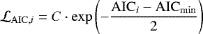
Fig. 1 TeV surface brightness maps of HESS J1534−571, HESS J1614−518, and HESS J1912+101 in Galactic coordinates. The maps were calculated with a correlation radius of 0.1°. An additional Gaussian smoothing with σ = 0.01°was applied to remove artifacts. The surface brightness is expressed in units of counts above 1 TeV, assuming a power law with index Γref. The inlets show the point spread function of the specific observations after applying the same correlation radius and smoothing, respectively. Top panel: HESS J1534−571, assumed Γref = 2.3. The green ellipse denotes the outer boundary of the radio SNR G323.7−1.0 from Green et al. (2014). Contours are 3, 4, 5, 6 σ significance contours (correlation radius 0.1°). Middle panel: HESS J1614−518, assumed Γref = 2.4. The green circle denotes the position and extent of 3FGL J1615.3−5146e from Acero et al. (2015). Contours are 5, 7, 9, 11 σ significance contours (correlation radius 0.1°). Bottom panel: HESS J1912−101, assumed Γref = 2.7. Contours are 3, 4, 5, 6, 7 σ significance contours (correlation radius 0.1°). |
2.4 TeV surface brightness maps
The morphological fits presented in Sect. 2.3 are based on a forward-folding technique. For the visualization of sky maps, depending on the properties of the data set, it may be necessary to correct acceptance changes in the sky maps themselves, specifically in the case of large extended sources. If H.E.S.S. sky maps are dominated by observations expressly targeted at the source of interest, the observations themselves ensure a nearly flat exposure and background level at and around the source, and γ-ray excess or significance maps are often an appropriate representation of the surface brightness of the sources. For the sources presented in this paper, however, all available observations of the respective source were used, whether they were part ofan observation of the particular source or a nearby source. This led to an uneven exposure with differences up to 30% on the regions of interest. Therefore, surface brightness maps were constructed for the three sources.
For this, flux maps were derived following the procedure described in H.E.S.S. Collaboration (2018f). A correlation radius of rint = 0.1° is used, Γref is chosen per source. To derive the surface brightness, the flux is divided by the area of the correlation circle  for every bin of the sky map. The grid size is 0.01° × 0.01°. From these maps, the integral flux of a source can be obtained by integrating over the radius of a region of interest, provided that the integration region is large compared to the psf. The surface brightness maps were checked for each of the three sources by comparing the integral flux from the maps with the respective result of the spectral analysis.
In Fig. 1, the TeV surface brightness maps of HESS J1534−571, HESS J1614−518, and HESS J1912+101 are shown using an energy threshold set to 1 TeV8. The assumed spectral indices for HESS J1614−518 and HESS J1912+101 were fixed independently of the spectral results discussed below and were taken from previous publications (Γref = 2.4 and 2.7; Aharonian et al. 2006b, 2008b). For HESS J1534−571, a typical value for Galactic sources, Γref = 2.3, was assumed. In fact, the assumed spectral index does not influence the appearance of the map. The reference flux, which is calculated based on the spectral index, only affects the overall scale of the displayed surface brightness (less than 5% for ΔΓ = 0.2; H.E.S.S. Collaboration 2018f). Radial and azimuthal profile representations of these surface brightness maps including the morphological fit results can be found in Appendix A.
2.5 Energy spectra
TeVenergy spectra for each of the new shells were derived using a forward-folding technique. Data were selected and analyzed according to the description in Sect. 2.2.2. On-source events are extracted from circular regions centered on the best-fit position and with radius Rout + R68% to ensure full enclosure (R68% ~0.07° is the 68% containment radius of the psf). Source, background, and effective area spectra with equidistant binning in log-space are derived runwise and are summed up. Power-law models
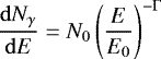 (5)
(5)
are convolved with the effective area and fit to the data. The lower fit boundary results from the image amplitude cut and corresponding energy bias cut. The upper fit boundary is dominated by the energy bias cut. The value E0 is the decorrelation energy of the fit, i.e., the energy where the correlation between the errors of Γ and N0 is minimal. All spectral parameters are listed in Table 4.
To display unfolded spectra, bins are background-subtracted and merged to have at least 2σ per bin, and spectra are divided by correspondingly binned effective areas. In Fig. 2, unfolded spectra and residuals between data and the power-law fits are shown. All three spectra are statistically compatible with power laws. Nevertheless, the spectra of the primary analysis of HESS J1534−571 and HESS J1912+101 as presented in Fig. 2 also show indications for curvature. A power-law model with exponential cutoff indeed better fits the data than a simple power law at the 3-4 σ level. However, the curvatures of the spectra (in particular of HESS J1912+101) are less pronounced in the cross-check analysis and are not significantly preferred there. The systematic errors that have been discussed in Sect. 2.2.2 not only lead to an error of the fitted power-law index value, but also to a distortion of the spectral shape. With the current spectral analysis, a more detailed description beyond a power law is not justified.
Spectral fit results from the power-law fits to the H.E.S.S. data.
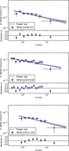 |
Fig. 2 Upper boxes show the H.E.S.S. energy flux spectra of HESS J1534−571, HESS J1614−518, and HESS J1912+101 (blue data points with 1 σ statistical uncertainties), respectively. The bin size is determined by the requirement of at least 2σ significance per bin. The solid blue lines with the gray butterflies (1 σ error of the fit) show the best fit power-law models from Table 4. The Bottom boxes show the deviation from the respective model in units of sigma, calculated as (F − Fmodel)∕σF. Systematic errors do not permit the application of more complex models to describe the data. |
3 Counterparts in radio continuum and GeV emission
3.1 Radio continuum emission
Several well-known high-energy emitting SNRs have only weak radio counterparts, such as the bright nonthermal X-ray and TeV-emitting SNRs RX J1713.7−3946 and RX J0852.0−4622; cf. e.g., Dubner & Giacani (2015). Confusion with thermal emission and Galactic background variations might therefore hamper the detection of radio counterparts of the new SNR candidates as well. We searched publicly available radio catalogs and survey data for counterparts of the new TeV sources.
3.1.1 The radio SNR candidate counterpart of HESS J1534−571
In 2014, Green et al. published a catalog of new SNR candidates that have been discovered using the Molonglo Galactic Plane Survey MGPS-2 (Murphy et al. 2007). The data were taken with the Molonglo ObservatorySynthesis Telescope (MOST) at a frequency of 843 MHz and with a restoring beam of  , where δ is the declination. The newly detected radio SNR candidate G323.7−1.0 is in very good positional agreement with the H.E.S.S. source. The extension and shell appearance of the two sources are in excellent agreement as well. To compare the two sources on more quantitative basis, radial profiles using elliptical annuli were extracted from the radio and TeV data.
In order to derive the profile of the radio emission observed in the MGPS-2 image at 843 MHz, a 1.2°-large sub-image from the original mosaic9 , centered at RA(J2000) = 233.572° and Dec(J2000) = -57.16° (i.e., the approximate barycenter of G323.7−1.0) was extracted. Each of the 28 sources listed in the MGPS-2 compact source catalog (Murphy et al. 2007) was masked out according to its morphological properties (minor/major axes and position angle). Two additional uncataloged source candidates and two extended sources were also removed. The RMS in the resulting source-subtracted image is 1.8mJy /beam. The flux density of G323.7-1.0 was measured after summing all the pixels inside an ellipse and correcting for the beam of 0.90′ × 0.75′ (FWHM). The ellipse is centered at the above-mentioned position and with the major and minor axes (51′ and 38′) as given in Green et al. (2014), and a position angle of 100° of the major axis (with respect to north), estimated from visual inspection of the image. The flux density amounts to (0.49 ± 0.08) Jy, compatible with the flux lower limit of 0.61Jy reported by Green et al. (2014). The difference is mostly due to one of the two uncataloged sources cited above that lie within the SNR candidate. It should be noted that the MOST telescope does not fully measure structures on angular scales larger than ~25′, so this flux density estimate must be considered as a lower limit, as explained in Green et al. (2014). The profile of the 843 MHz emission toward G323.7−1.0 shown in Fig. 3 was then derived from elliptical annuli of width 0.08° with the same parameters as above, after convolving the MGPS-2 image with the H.E.S.S. psf.
The TeV profile was derived following the procedure described in Appendix A, using elliptical annuli with the same parameters as used for the profile of the radio emission. The resulting TeV and radio radial profiles are shown in Fig. 3. The two profiles are statistically compatible with each other, confirming the association of the two sources as being due to the same object.
The total flux of G323.7−1.0 can also be used to provide a rough distance estimate of the SNR candidate, using the empirical surface brightness to source diameter (Σ − D) relation. Adopting ![Mathematical equation: ${\UpSigma}_{1\,\mathrm{GHz}} = 2.07 \times 10^{-17} \times D\left[\mathrm{pc}\right]^{-2.38}\,\mathrm{W\,m}^{-2}\,\mathrm{Hz}^{-1}\,\mathrm{sr}^{-1}$](/articles/aa/full_html/2018/04/aa30737-17/aa30737-17-eq13.png) (omitting the errors on the parameters) from Case & Bhattacharya (1998), S843 MHz = 0.49 Jy results in a distance estimate of 20 kpc. Individual source distance estimates have however typical errors of 40% (Case & Bhattacharya 1998). Moreover, as explained earlier, the radio surface brightness of G323.7−1.0 might be underestimated using the MOST data set. A two times higher radio flux would reduce the distance estimate to 15 kpc. Nevertheless, even a distance to HESS J1534−571 at the 10 kpc scale would imply a TeV luminosity substantially exceeding the values of the known TeV SNRs, as further discussed in Sect. 5.
(omitting the errors on the parameters) from Case & Bhattacharya (1998), S843 MHz = 0.49 Jy results in a distance estimate of 20 kpc. Individual source distance estimates have however typical errors of 40% (Case & Bhattacharya 1998). Moreover, as explained earlier, the radio surface brightness of G323.7−1.0 might be underestimated using the MOST data set. A two times higher radio flux would reduce the distance estimate to 15 kpc. Nevertheless, even a distance to HESS J1534−571 at the 10 kpc scale would imply a TeV luminosity substantially exceeding the values of the known TeV SNRs, as further discussed in Sect. 5.
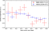 |
Fig. 3 Radial profile of HESS J1534−571 (H.E.S.S. TeV, blue points) and the SNR candidate G323.7−1.0 (MGPS-2 radio synchrotron at 843 MHz, red points) using elliptical annuli. The ratio of minor and major axes of the ellipse and the center position were both taken from Green et al. (2014). Since Green et al. (2014) do not quote a position angle for the ellipse, an angle of 100° of the major axis with respect to north was estimated from the radio map. The MGPS-2 image was convolved with the H.E.S.S. point spread function before extraction of the profile. Both profiles were normalized to have the same integral value. |
3.1.2 Radio continuum emission at the position of HESS J1912+101
In the sky area covered by HESS J1912+101, a radio SNR candidate G44.6+0.1 was discovered in the Clark Lake Galactic plane survey, at 30.9MHz (Kassim 1988). The SNR candidate status was confirmed through polarization detected at 2.7GHz (Gorham 1990). However, as already discussed in Aharonian et al. (2008b), the morphology and extension of the radio SNR candidate and the TeV source do not match. G44.6+0.1 is just covering part of the northwestern TeV shell and has an approximate elliptical shape of l × b = 41′ × 32′ 10.
The area of HESS J1912+101 was covered by the NRAO/VLA Sky Survey (Condon et al. 1998) at 1.4 GHz. Also, sky maps from the new Multi-Array Galactic Plane Imaging Survey (MAGPIS; Helfand et al. 2006) that combine VLA and Effelsberg data at 1.4 GHz were checked. The data suffer to some extent from side lobes from bright emission in the W49A region. No obvious counterpart to the TeV source was found by inspecting these data.
It is possible that the radio SNR candidate G44.6+0.1 is in fact part of a larger radio SNR corresponding to the TeV SNR candidate, but there is no further evidence from the data. Because of the lack of morphological correspondence between HESS J1912+101 and G44.6+0.1, the radio SNR candidate is not considered a confirmed counterpart to the TeV source, and G44.6+0.1 has therefore not been used to promote HESS J1912+101 from a SNR candidate to a confirmed SNR.
3.1.3 Search for radio continuum emission from HESS J1614−518
No cataloged radio SNR candidate exists in the field of HESS J1614−518. We inspected data from the Southern Galactic Plane Survey (SGPS; Haverkorn et al. 2006), obtained with the Australia Telescope Compact Array (ATCA) at 1.4 GHz, and from the MGPS-2 (Murphy et al. 2007) at 843 MHz. No obvious features spatially coincident with HESS J1614−518 were found, which is consistent with the findings by Matsumoto et al. (2008) using data from the Sydney University Molonglo Sky Survey (SUMSS; Bock et al. 1999). Much of the radio emission is associated with the HII regions to the western side of HESS J1614−518 and thus likely to be thermal in nature.
3.2 GeV emission with Fermi-LAT
Given the flux of the new TeV SNR candidates, a detection of source photons also in the adjacent GeVband covered with the Fermi-LAT instrument (Atwood et al. 2009) is plausible. Indeed, HESS J1614−518 has a known counterpart listed in the LAT source catalogs, namely 3FGL J1615.3−5146e/2FHL J1615.3−5146e. The source is classified in both catalogs as disk-like. Extension and position of the LAT source make it a clear counterpart candidate for HESS J1614-518; see Fig. 1. Together with the spectral match (see Fig. 4), we followed Acero et al. (2015) and Ackermann et al. (2016) and identified 3FGL J1615.3−5146e/2FHL J1615.3−5146e with HESS J1614−518. However, the identification currently does not add enough information to improve the astrophysical classification of the object.
Triggered by preliminary H.E.S.S. results on HESS J1534−571, Araya (2017) has recently shown that a disk-like GeV counterpart to HESS J1534−571 can be extracted from Fermi-LAT data as well. The GeV source position and size are in good morphological agreement with G323.7−1.0 and HESS J1534−571. The astrophysical classification of the object as a SNR from the TeV and radio data is not affected by the GeV data at this stage.
HESS J1912+101 does not have a published counterpart in the LAT band. Since the TeV source is extended and located in the Galactic plane, source confusion and emission from the Galactic plane might so far have prevented discovery of the source using the LAT instrument information alone. An analysis of all three objects using the TeV sources as prior information for a LAT analysis is ongoing.
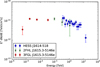 |
Fig. 4 TeV spectral energy flux of HESS J1614−518 plotted together with the GeV spectral energy flux of 2FHL J1614.3−5146e (Ackermann et al. 2016) and 3FGL J1614.3−5146e (Acero et al. 2015). The integral fluxes given in the Fermi-LAT catalogs were converted using the power-law models given in the catalogs. The energy of the flux points was determined by calculating the geometrical center of the energy boundaries in log-space. |
4 Counterpart searches using X-ray, infrared, and radio/sub-mm line emission, and pulsar catalogs
In this section, all MWL searches are reported that have not resulted in firm positive identifications with the new TeV sources. The following section provides details on these searches; in Sect. 5 the most relevant information for the discussion of the individual sources (specifically the X-ray results and potential gas densities at the object locations) is summarized.
4.1 Radio pulsars
The known, well-established TeV SNRs, such as RX 1713.7−3946, RX J0852.0−4622 (Vela Jr.), RCW 86, SN 1006, Cas A, and HESS J1731−347, are not associated with known rotation-powered radio pulsars. RCW 86 is very likely the SNR of a type Ia supernova (e.g., Broersen et al. 2014) without compact remainder. Cas A (Pavlov et al. 2000) and HESS J1731−347 (Klochkov et al. 2013, see also Tian et al. 2010; Halpern & Gotthelf 2010) host central compact objects (CCOs), i.e., neutron stars that are located close to the centers of the SNRs and whose X-ray emission is thermally driven; for RX 1713.7−3946 and RX J0852.0−4622, CCO candidates are known. However, that does not preclude other TeV SNRs with core collapse SN progenitors to be associated with radio pulsars. While the detection of possibly associated pulsars may not help in confirming the SNR nature of the new TeV shells, they may be used to elaborate possible SNR scenarios. Also, since energetic pulsars may drive TeV PWNe, it is important to check for these possible alternative object scenarios that may explain (part of) the TeV emission. In relic PWN scenarios, significant angular offsets between the powering pulsar and bulk of the TeV emission can be expected (e.g., H.E.S.S. Collaboration 2018d; Aharonian et al. 2006d, 2008a). Therefore, all radio pulsars listed in the ATNF catalog11 (Manchester et al. 2005), which are located inside a search radius of Rout + 0.3° around the fitted center of the TeV shell, were inspected.
4.1.1 The radio pulsar PSR J1913+1011 at the centerof HESS J1912+101
The rotation-powered pulsar PSR J1913+1011 is located close to the geometrical center of the TeV shell HESS J1912+101, at a distance of 2.7′. An association of that pulsar with the TeV source has been discussed in the context of a possible PWN scenario to explain the (lower-statistics) TeV source at the time of its discovery (Aharonian et al. 2008b). The pulsar has a spin-down power of Ė ≃2.9 ×1036 erg s-1, a (characteristic) spin-down age of τc ≃ 1.7 × 10⁵ yr, a spin period of 36 ms, and a distance of 4.5 kpc estimated from the dispersion measure (DM). The pulsar is in principle able to power a TeV PWN with a flux similar to HESS J1912+101 (Aharonian et al. 2008b). However, there is no known radio or X-ray PWN around PSR J1913+1011 (Gotthelf 2004; Chang et al. 2008), and the TeV morphology does not support a PWN scenario at all for the TeV source. Still, PSR J1913+1011 may be the remainder of the SN explosion that has created the putative TeV SNR; this is discussed in more detail in Sect. 5.4.
None of the other radio pulsars in the field of HESS J1912+101 are particularly compelling counterpart candidates to the TeV source. None of the pulsars show known radio or X-ray PWNe.
4.1.2 Radio pulsars around HESS J1614−518 and HESS J1534−571
None of the radio pulsars in the field of HESS J1614−518 are compelling counterpart candidates in a TeV PWN scenario. Also in this case, none of the pulsars show known radio or X-ray PWNe. In principle, in relic PWN scenarios high efficiencies of converting current spin-down luminosity into TeV luminosity (formally even above 100%, Aharonian et al. 2006d) can be present. It cannot be excluded that, for example, PSR J1613−5211 (τc ≈ 4 × 10⁵ yr, Ė ≈ 8 × 1033 erg s-1) drives the southwestern additional component in HESS J1614−518. However, there is currently no positive evidence to support such a hypothesis.
Three radio pulsars are located near HESS J1534−571, but energetics and distances make an association with HESS J1534−571 (in TeV PWN scenarios) unlikely.
4.2 Search for X-ray emission from the new TeV sources
All well-established TeV SNRs display strong extended nonthermal X-ray synchrotron emission from TeV electrons, typically in filamentary morphologies tracing the forward (and possibly reverse) shocks. Only a few TeV SNRs (such as Cas A and RCW 86) also exhibit strong thermal thin-plasma X-ray emission. All TeV SNRs but HESS J1731−347 are X-ray selected; X-ray emission from these objects was detected before the respective TeV detection. However, objects such as the new TeV SNR candidates that are located very close to the Galactic plane may not have been detected in soft X-ray surveys, such as that performed with the ROSAT satellite (energy range 0.1 keV – 2.4 keV), because of photoelectric absorption12 . Indeed, none of the three new TeV SNR candidates have obvious counterparts in ROSAT survey data. However, current and recent pointed X-ray instruments, such as XMM-Newton and Suzaku, may have the sensitivity to detect typical X-ray counterparts of TeV SNRs that have been detected at current TeV instrument sensitivities.
In the following, published and unpublished X-ray observations are reviewed that cover the TeV sources, in view of possible shell-like X-ray emission. In addition, X-ray (mostly point source) catalogs were checked, but (with the exception of XMMU J161406.0−515225 reviewed below) no compelling counterparts were found there.
4.2.1 Suzaku observations of HESS J1534−571
After the initial discovery of significant TeV emission from the position of HESS J1534−571 with H.E.S.S., the source was observed with Suzaku XIS (Mitsuda et al. 2007; Koyama et al. 2007) in four pointings with exposure times of 36.9 ks, 21.2 ks, 38.8 ks and 24.4 ks (observation IDs 508013010, 508014010, 508015010, and 508016010, respectively;PI A. Bamba). Further pointings to complete the coverage of the TeV source with Suzaku had already been approved, but could not be performed because of the failure of the satellite and subsequent decommissioning of the observatory.
For the analysis of the data, XSELECT and the Suzaku FTOOLS ver. 20 (part of HEASOFT ver. 6.13) were used. Particle-background subtracted, vignetting- and exposure-corrected mosaic images in the full band and in the harder band of 2 keV–12 keV were created. The harder band is expected to be more sensitive specifically to a nonthermal component of the potential X-ray counterpart because of Galactic absorption. In Fig. 5, this hard-band mosaic image is shown. No significant emission is detected from the source region in both mosaics. To estimate an X-ray upper limit from the area of the TeV source, spectra from a limited on- and an off-source region are derived; see Fig. 5 for the extraction regions that are defined with respect to the radio SNR boundary. In both spectra, there is a soft emission component whose characteristics are consistent with emission from hot thermal interstellar gas, and which is likely due to local X-ray foreground. In order to estimate an X-ray flux upper limit from the SNR, an additional (absorbed) power-law component was included in the on-spectrum model. The (unabsorbed) flux upper limit, derived from this power-law model (assuming two different photon indices Γ) and scaled to the area of the entire radio SNR, is 2.4 ×10⁻¹¹ erg cm-2 s-1 in the 2 keV–12 keV band for Γ = 2 and 1.9 ×10⁻¹¹ erg cm-2 s-1 in the 2 keV–12keV band for Γ = 3.
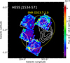 |
Fig. 5 Suzaku XIS mosaic of the pointings toward HESS J1534−571, in a hard band of 2 keV- 12 keV, using the XIS0 and XIS3 detectors. Point sources were not removed from the image. Contours denote the TeV surface brightness. The large solid ellipse denotes the outer boundary of the radio SNR. The small solid ellipse is the extraction region to derive an X-ray upper limit estimate from the SNR; the dashed ellipse is the corresponding background extraction region. |
4.2.2 XMM-Newton and Suzaku observations of HESS J1614-518
HESS J1614−518 was observed with Swift, Suzaku, and XMM-Newton in several pointings after the announcement of the TeV discovery (Aharonian et al. 2006b). Observations did not cover the entire TeV source but focused on the northeastern and southwestern components as well as on the central position. Matsumoto et al. (2008) and Sakai et al. (2011) reported on all Suzaku observations of the source and on the XMM-Newton data on the central area. Concerning point sources specifically in the central area, a possibly relevant source for this study is XMMU J161406.0−515225, at a distance of ~1′ from the geometrical center of the TeV shell13. Matsumoto et al. (2008) argued that the source might be an anomalous X-ray pulsar related to the TeV object. However, XMMU J161406.0−515225 has an optical point source counterpart, as already noted by Landi et al. (2006) based on the Swift-XRT detection of the source, and the source was classified as a star candidate in Lin et al. (2012).
Matsumoto et al. (2008) also reported on an extended X-ray source (Suzaku J1614−5141) with angular scale 5′, coincident with the northeastern component of HESS J1614−518. The X-ray absorption column is similar to that of XMMU J161406.0−515225, thus both objects could be related to the TeV source, at a distance scale to Earth on the order of 10 kpc using the X-ray absorption column as proxy (Sakai et al. 2011). To further probe potential diffuse X-ray emission from the region of HESS J1614−518, all XMM-Newton observations on the object have been examined (ObsID 0406650101 (northeast; PI Rowell), 0555660101 (southwest; PI Horns), and 0406550101 (central; PI Bussons), net exposure after event filtering (EPIC-MOS1/MOS2/pn) 21.0/19.9/13.7 ks, 17.0/17.6/6.5 ks, and 5.6/6.5/3.2 ks, respectively). Data were analyzed using XMMSAS ver. 14.0.0. First, mosaic images of the extended emission were created with ESAS. To this end, images for each observation were created and source detection was performed. Point sources detected by this procedure were masked out of the data. Then the quiet particle background and the soft proton contamination were modeled for each observation. All these images were combined and used to create background-subtracted, exposure-corrected mosaic images. Figure 6 shows these mosaics in two different energy bands, 0.3 keV–1.0 keV, and 3 keV–7 keV. The soft-band image demonstrates that the field specifically in the northeast is significantly contaminated by (soft) stray light from the nearby SNR RCW 103. The hard-band image shows that there is likely a hard diffuse X-ray emission component coincident with the northeastern TeV component of HESS J1614−518 with an angular scale of 20′, possibly indicating that the Suzaku source Suzaku J1614−5141 is more extended than seen in the Suzaku image.
To estimate the flux of the diffuse X-ray emission component, spectra were extracted for the entire hard emission region seen in the northwest above 3 keV (see circle in Fig. 6), and for a region excluding the strongest stray-light impact. Nearby background regions were selected to be representative of the expected background in the respective source extraction regions, and their spectra were fitted simultaneously. In general, a hard power-law component (Γ ≲ 2.0) is identified at the source position at high significance, but systematic errors are large specifically due to the stray-light impact.
A detailed assessment of the parameters of this diffuse X-ray component and its detection significance, including all systematic effects, is beyond the scope of this paper, as is a detailed comparison with the Suzaku result of Suzaku J1614−5141. The emission – if confirmed – fills a large portion of the FoVs of the EPIC instruments, and spectral analysis requires a detailed modeling of all background components. It seems very likely that the northwestern component of the TeV source HESS J1614−518 is accompanied by hard diffuse X-ray emission. However, the results are not sufficient to significantly improve the astrophysical classification of the object at this time.
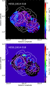 |
Fig. 6 XMM-Newton mosaics of the pointings toward HESS J1614−518, in a soft band (top panel, 0.3 keV–1.0 keV) and in a hard band (bottom panel, 3 keV–7 keV). Point sources were removed from the images. Contours denote the TeV surface brightness. The cross indicates the position of XMMU J161406.0−515225. The soft-band image is dominated by stray light from RCW 103 (northeastern arc feature). The hard-band image is dominated by a putative diffuse X-ray emission region coincident with the north component of the TeV source. The solid circle indicates an extraction area used to assess the spectrum for this diffuse component. Different background control regions (not shown) were used to estimate the systematic error induced by the background estimate. |
4.2.3 X-ray observations of HESS J1912+101
HESS J1912+101 is located at an angular distance of about 47′ to GRS 1915+105, making observations of the HESS J1912+101 region with X-ray satellites that are susceptible to stray light very difficult. As already discussed in Aharonian et al. (2008b), archival ASCA observations coincident with the HESS J1912+101 area are strongly affected by stray-light artifacts and are therefore of limited use to search for X-ray counterparts to HESS J1912+101. Archival Chandra data from observationstargeting at PSR J1913+1011 (and only covering the central region of HESS J1912+101) were analyzed by Chang et al. (2008) to explore a potential PWN scenario for HESS J1912+101 and to search for X-ray counterparts. None of the detected nine point sources seem particularly outstanding. No diffuse emission was detected. In view of the improved TeV morphology derived in this work, we reanalyzed the Chandra data (ObsId 3854). Comparison with the TeV image confirms the lack of compelling counterparts to HESS J1912+101, but also shows that there is no significant overlap of the Chandra exposure with the TeV-emitting shell.
At the moment, the shell of HESS J1912+101 remains largely unexplored at current pointed X-ray satellite sensitivity.
4.3 Infrared emission, possible associations with HII regions and stellar clusters
Infrared maps obtained with Spitzer at 24 μm, 8 μm, and 3.6 μm are used to illustrate the projected distribution of warm gas, HII regions, and stellar clusters in the field of the new TeV sources (Fig. 7). HESS J1534−571 is only partially covered by Spitzer data, therefore a Midcourse Space Experiment (MSX) map at 8.2 μm is used for that source.
The maps illustrate HII emission regions in apparent spatial coincidence with all three TeV sources. Such emission regions could consist of stellar wind material (e.g., Kothes & Dougherty 2007) from star-forming regions that could have also hosted the SNR progenitor stars. The formation of HII-emitting regions might also be triggered by the interaction with one or several SNRs. A morphological correlation between the IR and the TeV maps is not seen in the images and would also not necessarily be expected even if the TeV sources were associated with the HII emission regions.
The open stellar cluster Pismis 22 is located close to the geometrical center of HESS J1614−518. Its age is estimated tobe (40 ±15) Myr, at a distance of (1.0 ±0.4) kpc (Piatti et al. 2000). Pismis 22 could be the host of the progenitor star of a SNR, if the SNR interpretation of HESS J1614−518 is confirmed.
It is also interesting to evaluate the energy from the cluster as a whole. The total cluster mass is unconstrained, since most of the stars in the vicinity of Pismis 22, which are likely to be member stars, lack a spectral type determination. The expected kinetic energy in the system was estimated using the Starburst 99 cluster evolution model (Leitherer 2000, and references therein). The model results scale with the initial cluster mass MSC. The total kinetic energy including stellar winds and SNe over a time span of 40 Myr is 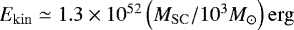 . Such a system with its output in kinetic energy would certainly leave its imprint in the cluster surroundings. Models such as that by Silich et al. (2005) predict a large cluster-wind driven void. Interestingly, the candidate HII region G331.628−00.926 with a radius of ~0.8° is encompassing in projection both HESS J1614−518 and Pismis 22. The current cluster luminosity at the adopted age of 40 Myr is Lkin (t = 40 Myr) ≃ 5.2 × 1036MSC∕10 M⊙ erg s−1. Therefore, a fraction of this luminosity would be sufficient to explain the TeV luminosity of HESS J1614−518 in terms of its energy requirement. Lacking any observational evidence, this possibility remains hypothetical for the moment.
In conclusion, the presented IR data themselves do not contribute to the astrophysical identification of the new TeV sources, but the HII and stellar data add information to a possible SNR scenario for HESS J1614−518.
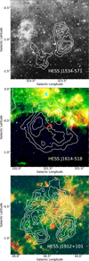 |
Fig. 7 Archival infrared images toward the fields of the three TeV sources. Top panel: MSX (Price et al. 2001) image of the region toward HESS J1534-571, at 8.28 μm. Middle and bottom panels: three-color Spitzer images toward HESS J1614−518 and HESS J1912+101, respectively. Red, green, and blue colors indicate 24 μm (MIPSGAL, Carey et al. 2009), 8 μm, and 3.6 μm (GLIMPSE, Churchwell et al. 2009) emission, respectively. Color scales were adjusted individually to emphasize the structures in the images. Contours denote the TeV surface brightness of the respective source. The circle at the center of HESS J1614−518 denotes the position and extension of Pismis 22 (Morales et al. 2013). |
4.4 Atomic and molecular gas density around the sources
Archival radio and sub-mm atomic and molecular line data were investigated to search for signatures of gas associations corresponding to the new shell-type γ-ray sources. Voids in HI data would be suggestive of stellar wind bubbles blown by massive progenitor stars, while arcs of HI emission or asymmetric spectral line profiles may be attributable to gas shocked by a SNR. Such features would deliver a SNR kinematic distance solution. A positive correlation between γ-ray emission and gas density would be suggestive of a spatial connection that would yield a kinematic distance estimate, while at the same time lending support to the hypothesis that a γ-ray source is of hadronic origin (typically better seen in molecular gas, e.g., toward SNR W28; Aharonian et al. 2008a).
Nanten CO(1-0) data (Matsunaga et al. 2001) are available toward the new TeV shells and have an angular resolution of ~3′. Additionally, Galactic Ring Survey (GRS; Jackson et al. 2006) 13 CO(1-0) and CS(2-1) data with an angular resolution of 46′′ are available toward HESS J1912+101 for molecular gas components with positive velocities. To trace atomic gas (as opposed to the aforementioned molecular gas tracers) toward the new H.E.S.S. shells, ~2′-resolution Southern Galactic Plane Survey (SGPS; McClure-Griffiths et al. 2005) HI data are available for the southern sources HESS J1534−571 and HESS J1614−518, while HESS J1912+101 is covered by the 1′ resolution HI data from the VLA Galactic Plane Survey (VGPS; Stil et al. 2006).
Longitude-velocity plots of Columbia CO(1-0) data (Dame et al. 2001) are used to illustrate the large-scale Galactic structure toward the new TeV shells in Fig. 8. For translating radial velocities relative to the local standard of rest (LSR) into distance estimates, the prescriptions of Vallée (2008, 2013) are used. In general, there are often ambiguities in associating specific gas components with specific Galactic arms, but associations indicated in Fig. 8 are considered the most likely according to current literature. HESS J1534−571 and HESS J1614−518 are within 8°of each other and are both in projection coincident with the Sagittarius-Carina, Scutum-Crux, and Norma-Cygnus arms (Vallée 2008, 2013). Regarding HESS J1912+101, the CO data show two velocity components meeting near the tangent point of the Sagittarius arm (Vallée 2008, 2013), so significant uncertainty exists in distance estimations to specific atomic and molecular gas components there.
CO, 13CO, CS, and HI spectral profiles toward the three new TeV shell sources are shown in Fig. 9. Multiple line-of-sight gas components may potentially be associated with the TeV sources. No unambiguous match has been found in the comparisons of the ISM skymaps with the TeV sky maps. For these comparisons, CO and HI sky maps were produced in a series of velocity bands covering the entire velocity range shown in Fig. 9, and were then compared to the TeV maps. The only noteworthy indication found in this investigation is a void or dip in the SGPS HI data set centered on HESS J1614−518 in the distance range between 1.2 kpc and 1.5 kpc (vlsr = -15 km s-1 to -22 km s-1)(see Fig. B.2 top left panel), which may suggest an association with HESS J1614−518. The HI emission appears as a partial shell toward the rim of the TeV source, hinting at the possibility of a blown-out bubble related to a shell-type SNR (from the progenitor star) or to an alternative central energy source. This distance range encompasses that of the Pismis 22 open cluster (cf. Sect. 4.3), and thus may signal the mechanical influence of this cluster on the atomic ISM, in a similar fashion to the HI feature identified by Kothes & Dougherty (2007) toward the WR cluster Westerlund 1, which is possibly associated with a TeV γ-ray source (Abramowski et al. 2012).
Since no unambiguous association was found for any of the three sources, two representative distances with a possible gas match have been chosen per source. The goal is to demonstrate that reasonable hadronic emission scenarios can be constructed for each of the sources, using possible target gas densities in which the sources could be embedded (deviating from the canonically assumed particle density of 1 cm−3). No attempt was made to quantify whether the matches themselves are statistically significant, from the gas data alone. The associations are detailed in Appendix B.2. The way gas densities are derived is explained in Appendix B.3. Results are shown in Table 7 and are discussed further in the following discussion section.
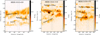 |
Fig. 8 Longitude-velocity plots of Columbia CO(1-0) data (Dame et al. 2001), integrated over a latitudinal range consistent with HESS J1912+101, HESS J1614−518, and HESS J1534−571 (left, middle, and right, respectively). The longitudinal extent of each of these SNRs is indicated by dashed lines. The names of Galactic arms are overlaid onto the approximate corresponding map locations, following Vallée (2008). |
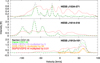 |
Fig. 9 Average Nanten/Columbia CO(1-0) (Matsunaga et al. 2001; Dame et al. 2001) data within circular regions encompassing HESS J1534−571 ([l,b,r] = [323.70, −1.02,0.4]), HESS J1614−518 ([l,b,r] = [331.473,−0.601,0.42]), and HESS J1912+101 ([l,b,r] = [44.46, −0.13,0.49]). HI data are also shown for all sources (SGPS/VGPS McClure-Griffiths et al. 2005; Stil et al. 2006), while GRS 13 CO(1-0) and CS(2-1) (Jackson et al. 2006) data are shown for HESS J1912+101. The CS(2-1) feature at 9.5 km s-1 in the bottom image is likely an artifact caused by an offset in one frequency channel. |
5 Discussion
From the presented morphological studies using H.E.S.S. data, the three TeV sources HESS J1534−571, HESS J1614−518, and HESS J1912+101 have been classified as SNR candidates. The identification of HESS J1534−571 with the radio SNR candidate G323.7−1.0 has led to the classification of HESS J1534−571 as SNR. The nondetection of radio synchrotron emission from the other two sources is not in conflict with the SNR hypothesis for these objects. The GeV counterpart situation (i.e., the Fermi-LAT counterparts for HESS J1534−571 and HESS J1614−518 and no known counterpart for HESS J1912+101) is compatible with the respective TeV fluxes but does not contribute to the classification of the sources. Table 5 gives an overview of the confirmed (HESS J1534−571) and possible(HESS J1614−518, HESS J1912+101) association scenarios and corresponding distance scale estimates, as discussed in Sects. 3 and 4.
For the new SNR candidates, Table 7 lists derived parameters (diameter, luminosity) for three different assumed distances, namely a generic 1 kpc distance and the distances listed in Table 5. The values can be compared to the corresponding parameters of known TeV SNR shells as shown in Table 6. On average, the photon indices of the new shells seem slightly softer than those of the known SNR shells. However, for individual sources the respective errors are too large to draw any conclusion. Luminosities and diameters of the new SNR candidates are compatible with the known SNR shells for assumed nearby distances of ~1 kpc. The new sources would be larger and more luminous than the known SNRs already for moderate distances of ~3 kpc. Distances at a 8 kpc…10 kpc scale are either disfavored or would indicate a different, substantially more luminous new TeV SNR source population. At these distances, the physical diameters of the SNRs would also be substantially larger than those of the known TeV SNRs, and well beyond a cutoff in the general SNR diameter distribution at ~60 pc as derived from SNRs in the Magellanic clouds and M 33 (see Badenes et al. 2010, and references therein). If this cutoff is indeed attributed to a lower limit in the ambient density distribution, as argued by Badenes et al. (2010), then outliers beyond ~60 pc (e.g., the new TeV SNRs if indeed at 8…10 kpc distance) might be connected to remnants of core collapse SNe with modified ambient medium (cf. the discussion in Badenes et al. 2010). This would be consistent with arguments that have been made to explain the sizes of, for example, the TeV SNRs RX J1713.6−3946 and HESS J1731−347. To investigate whether this is a realistic scenario and whether specific wind progenitor bubbles could lead to SNR sizes at the ~100 pc diameter scale is beyond the scope of this paper.
Overview of confirmed (HESS J1534−571) and possible (HESS J1614−518, HESS J1912+101) association scenarios.
Parameters of known TeV SNR shells.
Parameters of the new TeV SNR candidates, assuming a generic 1 kpc distance and two other distances coming from possible association scenarios.
5.1 TeV emission from leptons or protons
One of the fundamental questions of SNR research is what fraction of the ejecta energy goes into thermal (typically X-ray-emitting) plasma, and what fraction goes into a nonthermal component consisting of relativistic particles (best visible in hard X-rays and high to very high γ-ray energies). The energy share between relativistic hadrons and leptons and the maximum particle energy determine whether SNRs contribute significantly to the generation of Galactic CRs up to the knee in the CR particle spectrum. Unlike other identified TeV SNRs, the new TeV sources do not have confirmed X-ray counterparts. The lack of thermal X-rays may be interpreted as a signature for low density environment and therefore leptonically dominated TeV emission processes. However, the absorption column to the new sources is not constrained from the TeV data. Depending on the actual distance to the source, and on the temperature and density of the emitting plasma, foreground absorption might have prevented detection of soft thermal X-rays, for example, in the ROSAT survey. There is also sufficient uncertainty about which level of thermal heating could be expected, for example, in a clumpy environment (e.g., Gabici & Aharonian 2014).
Nonthermal X-rays above ~2 keV are however expected in shock-compressed (and possibly further amplified by CR streaming) magnetic fields, if the TeV emission stems from relativistic electrons. As discussed in Sect. 4.2.2, within the presented study it has not been possible to constrain conclusively the hard X-ray emission likely associated with HESS J1614−518. HESS J1912+101 lacks sensitive pointed X-ray coverage. The nondetection of X-ray emission from HESS J1534−571 from a (partial) Suzaku coverage seems interesting at first glance, but may not yet be constraining (see next section).
5.2 HESS J1534−571
A confirmed upper limit on the X-ray emission from HESS J1534−571 in the 2keV – 10 keV range would present the first case of a TeV SNR without an X-ray counterpart at current satellite sensitivity. The absence of nonthermal X-ray emission is generally used to challenge the interpretation that a relativistic electron population in the source is responsible for the γ-ray emission because a certain minimum level of X-ray synchrotron emission is expected in a minimum Galactic magnetic field of 3 μG. More quantitatively, a ratio R = Fγ(1 − 10 TeV)∕FX(2 − 10 keV) can be defined following, for example, Yamazaki et al. (2006). Young known SNRs have a ratio R significantly less than 2, while R larger than 2 couldbe indicative of a largely evolved (so-called X-ray dark) SNR, whose TeV emission should then be dominated by proton-induced π0 -decay (Yamazaki et al. 2006). Assuming the current Suzaku limit holds for the entire HESS J1534−571 shell, R > 0.25. A detectionof nonthermal X-ray emission is therefore within reach if HESS J1534−571 is similar to other TeV SNRs. To establish a sensitive upper limit (indicating that the TeV emission stems from protons) is however challenging even for current X-ray instruments because of the large extension of the source.
The TeV data do not permit a distance estimate to HESS J1534−571 (as for any of the new sources). Using the SNR radio surface brightness to diameter (Σ − D) relation, the distance to G323.7−1.0 is estimated tobe 20 kpc (cf. Sect. 3.1.1). However, individual distances derived from Σ − D have large errors, which are typically 40% for the normal SNR population. Assuming that the radio counterpart of HESS J1534−571 is similarly underluminous as that of RX J1713.7−3946 with respect to its Σ − D expectation value at 1 kpc would reduce the distance estimate of G323.7−1.0 to ~ 5 kpc. This distance would imply a TeV luminosity of HESS J1534−571 in reasonable agreement with TeV luminosities from the other known TeV SNRs (cf. Table 6).
5.3 HESS J1614−518
Also for HESS J1614−518, distance estimates only come from possible associations. One such is the open stellar cluster Pismis 22, located close to the center of HESS J1614−518 (cf. Sect. 4.3), which may have hosted the SNR progenitor star. The distance estimate to this stellar cluster, (1.0 ± 0.4) kpc (Piatti et al. 2000), is in accordance with a possible HI void seen in projection at a distance of 1.2 kpc…1.5 kpc (cf. Sect. 4.4).
Another association was suggested by Sakai et al. (2011). The X-ray source XMMU J161406.0−515225, a point source close to the center of HESS J1614−518, and the diffuse source Suzaku Src A defined in Matsumoto et al. (2008) may be associated with the TeV source (cf. Sect. 4.2.2). Using the X-ray absorption column as proxy, a rough distance scale of 10 kpc was estimated, which is likely compatible with a possible spiral arm association at ~5.5 kpc distance (cf. Appendix B.2).
5.4 HESS J1912+101
As discussed in Sect. 4.1.1, the pulsar PSR J1913+1011 located at the center ofHESS J1912+101 may be the remainder of the SN explosion that has created the putative TeV SNR. At a distance of 4.5 kpc estimated from the dispersion measure of the pulsar, the TeV shell size would then correspond to a SNR radius of ~40 pc. As for all sources presented in the paper, the TeV shell morphology implies that particle acceleration to supra-TeV energies is likely still ongoingor has been ongoing until the recent past; otherwise, diffusion of the no longer confined particles would have washed out the current morphology. To provide the necessary high shock speed, the age of the putative SNR HESS J1912+101 should then be at least an order of magnitude lower than the characteristic age of the pulsar (τc ≃ 1.7 × 10⁵ yr), if the association with PSR J1913+1011 was confirmed. To maintain the association, the birth spin period of the pulsar therefore needs to have been close to the current spin period, which is in principle possible.
5.5 Proton scenarios
Assuming that the γ-ray emission seen in the TeV regime is purely due to hadronic processes, an estimate of the fraction of the SNR explosion energy going into accelerated CR protons can be given.
In the delta-function approximation (Kelner et al. 2006), γ-ray photons of energy Eγ are produced by protons with energy Ep = 10 × Eγ. Following the arguments in Aharonian et al. (2006c), the total energy in accelerated protons in the 10 TeV–100 TeV range can be estimated from the γ-ray luminosity in the range 1 TeV–10 TeV, using
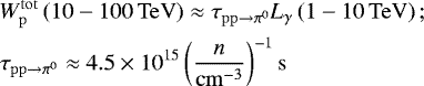 (6) (7)
is the characteristic cooling time of protons by π0 production and
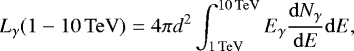 (8)
(8)
where d is the distance to the source and  , as described in Sect. 2.2. The values N0,1 TeV and Γ are derived from the fit to the TeV data as presented in Table 4.
Knowing 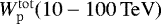 and assuming a power-law spectrum forthe accelerated protons (dNp∕dE = NpE−α, with α = Γ and Np a normalization factor),
  can be calculated in an arbitrary proton energy range. It is assumed that the proton energy spectrum can be described by a broken power law with a break energy at 10 TeV,
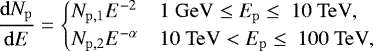 (9)
(9)
which is roughly compatible with the TeV spectra of all three new shell sources and the GeV spectrum of the Fermi-LAT source associated with HESS J1614−518.
To illustrate the possible energy contents in accelerated protons, three scenarios are given in Table 7 for each source. The first is a generic case with a distance of 1 kpc and a target gas density of 1 cm −3. The other two are derived from the possible gas association scenarios as introduced in Sect. 4.4 and Appendix B.2 (cf. Table 5), where error ranges are propagated from the estimated ranges of gas densities. The table lists both the energy contents of the protons in the TeV-emitting energy range and for an extrapolated spectrum down to 1 GeV. The latter values show that the available data are compatible with the expected energy content of 10% of 1051 erg for assumed nearby distances of ~1 kpc and for moderate distances of ~3 kpc. Distances at a 8 kpc…10 kpc scale and beyond are disfavored in hadronic emission scenarios.
6 Conclusions
A dedicated search for new SNR shells in the H.E.S.S. Galactic plane survey data has revealed three new SNR candidates. HESS J1534−571 was confirmed as a SNR from an identification with a radio SNR candidate, while HESS J1614−518 and HESS J1912+101 remain SNRcandidates for the time being. From the current knowledge of multiwavelength data, both leptonic or hadronic (or a blend of both) TeV emission scenarios are possible. Distances to the objects on the 8 kpc to 10 kpc scale or beyond seem unlikely from a comparison of the TeV fluxes to the luminosities of known TeV SNR shells. Such large distances are also difficult to accommodate in hadronic TeV emission scenarios. Distances to the new objects at the 1 kpc to 3 kpc scale seem most likely, while distances below the 1 kpc scale might indicate unusual properties regarding their X-ray emissivity.
The analysis has demonstrated that current Imaging Atmospheric Cherenkov Telescope Arrays have the power to discover new SNRs. The future Cherenkov Telescope Array will substantially increase the available sensitivity to detect TeV SNRs in the entire Galaxy. Source confusion may however become a more severe problem than in the study presented here.
Acknowledgements
The support of the Namibian authorities and of the University of Namibia in facilitating the construction and operation of H.E.S.S. is gratefully acknowledged, as is the support by the German Ministry for Education and Research (BMBF), the Max Planck Society, the German Research Foundation (DFG), the Alexander von Humboldt Foundation, the Deutsche Forschungsgemeinschaft, the French Ministry for Research, the CNRS-IN2P3 and the Astroparticle Interdisciplinary Programme of the CNRS, the UK Science and Technology Facilities Council (STFC), the IPNP of the Charles University, the Czech Science Foundation, the Polish National Science Centre, the South African Department of Science and Technology and National Research Foundation, the University of Namibia, the National Commission on Research, Science & Technology of Namibia (NCRST), the Innsbruck University, the Austrian Science Fund (FWF), and the Austrian Federal Ministry for Science, Research and Economy, the University of Adelaide and the Australian Research Council, theJapan Society for the Promotion of Science, and by the University of Amsterdam. We appreciate the excellent work of the technical support staff in Berlin, Durham, Hamburg, Heidelberg, Palaiseau, Paris, Saclay, and in Namibia in the construction and operation of the equipment. This work benefited from services provided by the H.E.S.S. Virtual Organisation, supported by the national resource providers of the EGI Federation. The shell search performed on the entire HGPS data set as presented in Sect. 2.3 employed Gammapy routines as presented in Donath et al. (2015). This research has made use of the VizieR catalog access tool, CDS, Strasbourg, France. The original description of the VizieR service was published in Ochsenbein et al. (2000). This research hasmade use of the SIMBAD database, operated at CDS, Strasbourg, France (Wenger et al. 2000).
Appendix A TeV surface brightness profiles
After fittingthe two-dimensional models to the TeV count sky maps as described in Sect. 2.3, profiles were extracted in units of surface brightness from the observations and the models to verify the fit results. The azimuthal profiles were also used to quantify possible deviations of the source maps from azimuthal symmetry, as discussed in Sect. 2.3.4. The measured profiles were derived from the uncorrelated excess maps of the dedicated source analysis (cf. Sect. 2.2.2). Surface brightness profiles are derived by dividing the excess within the respective profile bin area by the expected counts derived from the simulated instrument response (H.E.S.S. Collaboration 2018f) and by the area of the profile bin. The profiles are shown in Fig. A.1. Shell and Gaussian model profiles were scaled to corresponding surface brightness units.
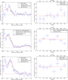 |
Fig. A.1 TeV surface brightness profiles of HESS J1534−571, HESS J1614−518, and HESS J1912+101. Left column: radial profiles; right column: azimuthal profiles, respectively. The shell models and Gaussian models (shown in the left panels) are from fits to the data. The point source simulation shown in the left panels is derived from the sum of three Gaussians fitted to a simulated point source as it would appear in the actual data set (cf. Sect. 2.3.1), arbitrarily normalized for good visual representation. The value of Θ in the azimuthal profiles represents the angle with respect to the Galactic latitude. The first wedge is at Θ = 0 ° , following wedges are added counter-clockwise. The angle with respect to north in equatorial coordinates is represented by Θ′. |
For the radial profiles of the observed data, circular annuli around the centroids of the shell models, and with a width of 0.04° were used. The profiles of the shell and Gaussian models were derived analogously but with a two times finer binning. As expected from the fitting results, the shell model describes the data best in all three cases. A positive excess is visible in the profile of HESS J1614−518 from ~0.7° outward. This emission stems from the nearby source HESS J1616−508 and is taken into account in the fit procedure with an additional Gaussian component in the model of HESS J1614−518, both when fitting the Gaussian model and the shell model. The separation of both sources is large enough so that the emission of HESS J1616−508 does not significantly affect the spectral results of HESS J1614−518.
To derive the azimuthal profiles, the sources were divided into eight wedges of equal angular size with outer radii of Rout, respectively, and with inner radii slightlysmaller than Rin to increase the photon statistics of the profiles (because of the projection of the shells, the peak of the radial profiles is close to Rin). In the azimuthal model profile of HESS J1614−518, the modeled emission of HESS J1616−508 is barely visible above the flat shell profile.
Appendix B Details on gas association
B.1 SNRs associated with molecular clouds
Besides the well-identified TeV SNR shells, several resolved TeV sources are likely driven by SNR particle acceleration processes as well, but the TeV morphology is determined by molecular clouds close to or partially coincident with the SNRs. The underlying assumption is that TeV emission is created in these clouds through collisions of SNR-accelerated hadronic particles with dense gas. Examples comprise IC 443, W51C, CTB 37A, or Tycho’s SNR (Albert et al. 2007; Fiasson et al. 2009; Aharonian et al. 2008c; Acciari et al. 2011). The firm confirmation of such a scenario is often challenging. The TeV images, which are statistically limited, need to be correlated with sub-mm line data (tracing molecular gas), which provide moderate distance resolution and thus a large number of possible projections over different distance ranges, resulting in a large number of trials. In some cases, possible alternative PWN scenarios also exist for the interpretation of the TeV emission. Because of the expected ambiguities as experienced from the analysis of these known sources, molecular gas information is not used as criterion for the morphological identification of the TeV sources as SNR candidates for the work presented in this paper.
B.2 Choices for gas/spiral arm associations for the new TeV shells
For HESS J1534−571, one gas match around 3.5 kpc (right panels of Fig. B.1) and one around 8 kpc (left panels of Fig. B.1) were chosen.The latter distance might be compatible with the distance estimate of 20 kpc derived for the radio counterpart from the Σ − D relation, given the uncertainties of the method. No attempt was made to construct a case with a distance far beyond the Galactic center distance.
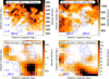 |
Fig. B.1 HESS J1534−571. HI (top panels) and CO (bottom panels) intensity images toward the direction of HESS J1534−571 in velocity ranges as given on the images. HI data are from the Southern Galactic Plane Survey (McClure-Griffiths et al. 2005), CO data are from Nanten (Matsunaga et al. 2001). The slices in the left two panels correspond to a location in the Norma-Cygnus arm at a distance of 8 kpc, while the right two panels are from a location in the Scutum-Crux arm at a distance of 3.5 kpc. |
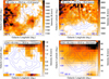 |
Fig. B.2 HESS J1614−518. HI (top panels) and CO (bottom panels) intensity images toward the direction of HESS J1614−518, in velocity ranges as given on the images. HI data are from the Southern Galactic Plane Survey McClure-Griffiths et al. (2005); CO data are from Nanten (Matsunaga et al. 2001). The slices in the left two panels correspond to a location in the Sagittarius-Carina arm at a distance of 1.5 kpc, while the right two panels are from a location in the Norma-Cygnus arm at a distance of 5.5 kpc. The HI images at the velocity range of -30 km s-1 to -12 km s-1 indicate a possible void in the gas in directional coincidence with HESS J1614−518. At the center of this position and in compatible distance to Earth, the stellar cluster Pismis 22 is located. |
For HESS J1614−518, the HI void distance range between 1.2 kpc and 1.5 kpc as discussed in Sect. 4.4 has been chosen as a first possibility (left panels of Fig. B.2). The distance is compatible with the estimated distance to Pismis 22 by Piatti et al. (2000). As a second possibility, a 5.5 kpc distance was selected (right panels of Fig. B.2). The integrated proton column density to this distance from atomic and molecular hydrogen (3–4 × 1022 cm−2) is in fact of similar order to the absorption column NH ~ 1–2 × 1022 cm−2 that has been derived for XMMU J161406.0−515225 and Suzaku J1614−5141 (Sakai et al. 2011), which were suggested by these authors to possibly be associated with HESS J1614−51814.
Regarding HESS J1912+101, the dispersion distance of the possibly associated pulsar PSR J1913+1011 (cf. Sect. 4.1.1) of ~4.5 kpc is consistentwith the range of distances expected to be found within the Sagittarius arm in this direction. One of the two distance ranges was therefore chosen as the approximate mid-range of the Sagittarius arm line-of-sight velocities, matching 4.5 kpc (right panels of Fig. B.3). As a second possibility, another possible match within the Perseus arm at 10 kpc distance was chosen (left panels of Fig. B.3).
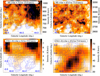 |
Fig. B.3 HESS J1912+101. HI (top panels) and CO (bottom panels) intensity images toward the direction of HESS J1912+101, in velocity ranges as given on the images. HI data are from the VLA Galactic Plane Survey (Stil et al. 2006); CO data are from Nanten (Matsunaga et al. 2001). The slices in the left two panels correspond to a location in the Perseus arm at a distance of 10 kpc, while the right two panels are from a location in the Sagittarius-Carina arm at a distance of 4.5kpc. |
Gas tracers toward HESS J1912+101 were also recently investigated by Su et al. (2017). The authors have argued that 12 CO and HI line velocity features found in their data are indicative of shock-gas interaction, possibly originating from an old ( ~105 yr) SNR that could be associated with HESS J1912+101. Here, we note that the line velocity range of the bulk of the corresponding molecular gas (around vlsr ≃ 60 km s−1) is consistent with one of the two line velocity ranges chosen for HESS J1912+101 in this work.
All distances used were again estimated using figures from Vallée (2008, 2013).
B.3 Gas density estimates for the new TeV shells
In order to derive the total (atomic and molecular) ISM density possibly associated with each respective TeV source, the gas emission is assumed to come from a homogeneous cylindrical region defined by the SNR outer boundary for a given velocity range. Molecular densities are derived using the CO-to-H2 mass conversion factor ![Mathematical equation: $1.5 \times 10^{20}\,\mathrm{cm}^{-2}\,[\mathrm{K\,km\,s}^{-1}]^{-1}$](/articles/aa/full_html/2018/04/aa30737-17/aa30737-17-eq21.png) from Strong et al. (2004), while atomic H densities are derived using the HI brightness temperature to column density conversion factor of
from Strong et al. (2004), while atomic H densities are derived using the HI brightness temperature to column density conversion factor of ![Mathematical equation: $1.8 \times 10^{18}\,\mathrm{cm}^{-2}\,[\mathrm{K\,km\,s}^{-1}]^{-1}$](/articles/aa/full_html/2018/04/aa30737-17/aa30737-17-eq22.png) from Dickey & Lockman (1990). For each case, a density range was calculated by assuming that the line-of-sight thickness is between a value either equal to the SNR candidate diameter or equal to the approximate thickness of a Galactic arm (0.5 kpc). The first (upper) density value is therefore in all likelihood an overestimation. Moreover, it cannot be excluded that the density at the position of the source is well below the second (lower) value, for example, if the SNR is fully contained in a wind-blown bubble of the progenitor star. In such a case, however, a hadronic TeV emission scenario is anyway unlikely. Results are shown in Table 7.
from Dickey & Lockman (1990). For each case, a density range was calculated by assuming that the line-of-sight thickness is between a value either equal to the SNR candidate diameter or equal to the approximate thickness of a Galactic arm (0.5 kpc). The first (upper) density value is therefore in all likelihood an overestimation. Moreover, it cannot be excluded that the density at the position of the source is well below the second (lower) value, for example, if the SNR is fully contained in a wind-blown bubble of the progenitor star. In such a case, however, a hadronic TeV emission scenario is anyway unlikely. Results are shown in Table 7.
References
- Abramowski, A., Acero, F., Aharonian, F., et al. 2012, A&A, 537, A114 [NASA ADS] [CrossRef] [EDP Sciences] [Google Scholar]
- Acciari, V. A., Aliu, E., Arlen, T., et al. 2011, ApJ, 730, L20 [NASA ADS] [CrossRef] [Google Scholar]
- Acero, F., Aharonian, F., Akhperjanian, A. G., et al. 2010, A&A, 516, A62 [NASA ADS] [CrossRef] [EDP Sciences] [Google Scholar]
- Acero, F., Ackermann, M., Ajello, M., et al. 2015, ApJS, 218, 23 [Google Scholar]
- Ackermann, M., Ajello, M., Atwood, W. B., et al. 2016, ApJS, 222, 5 [NASA ADS] [CrossRef] [Google Scholar]
- Aharonian, F., Akhperjanian, A., Barrio, J., et al. 2001, A&A, 370, 112 [NASA ADS] [CrossRef] [EDP Sciences] [Google Scholar]
- Aharonian, F. A., Akhperjanian, A. G., Beilicke, M., et al. 2002, A&A, 395, 803 [NASA ADS] [CrossRef] [EDP Sciences] [Google Scholar]
- Aharonian, F. A., Akhperjanian, A. G., Aye, K.-M., et al. 2004, Nature, 432, 75 [NASA ADS] [CrossRef] [PubMed] [Google Scholar]
- Aharonian, F., Akhperjanian, A. G., Bazer-Bachi, A. R., et al. 2006a, A&A, 457, 899 [NASA ADS] [CrossRef] [EDP Sciences] [Google Scholar]
- Aharonian, F., Akhperjanian, A. G., Bazer-Bachi, A. R., et al. 2006b, ApJ, 636, 777 [NASA ADS] [CrossRef] [Google Scholar]
- Aharonian, F., Akhperjanian, A. G., Bazer-Bachi, A. R., et al. 2006c, A&A, 449, 223 [NASA ADS] [CrossRef] [EDP Sciences] [Google Scholar]
- Aharonian, F., Akhperjanian, A. G., Bazer-Bachi, A. R., et al. 2006d, A&A, 460, 365 [NASA ADS] [CrossRef] [EDP Sciences] [Google Scholar]
- Aharonian, F., Akhperjanian, A. G., Bazer-Bachi, A. R., et al. 2007a, A&A, 467, 1075 [NASA ADS] [CrossRef] [EDP Sciences] [Google Scholar]
- Aharonian, F., Akhperjanian, A. G., Bazer-Bachi, A. R., et al. 2007b, ApJ, 661, 236 [NASA ADS] [CrossRef] [Google Scholar]
- Aharonian, F., Akhperjanian, A. G., Barres de Almeida, U., et al. 2008a, A&A, 477, 353 [NASA ADS] [CrossRef] [EDP Sciences] [Google Scholar]
- Aharonian, F., Akhperjanian, A. G., Barres de Almeida, U., et al. 2008b, A&A, 484, 435 [NASA ADS] [CrossRef] [EDP Sciences] [Google Scholar]
- Aharonian, F., Akhperjanian, A. G., Barres de Almeida, U., et al. 2008c, A&A, 490, 685 [NASA ADS] [CrossRef] [EDP Sciences] [Google Scholar]
- Akaike, H. 1974, IEEE Trans. Autom. Control, 19, 716 [NASA ADS] [CrossRef] [MathSciNet] [Google Scholar]
- Albert, J., Aliu, E., Anderhub, H., et al. 2007, ApJ, 664, L87 [NASA ADS] [CrossRef] [Google Scholar]
- Araya, M. 2017, ApJ, 843, 12 [NASA ADS] [CrossRef] [Google Scholar]
- Aschenbach, B. 1995, in The Physics of the Interstellar Medium and Intergalactic Medium, eds. A. Ferrara, C. F. McKee, C. Heiles, & P. R. Shapiro, ASP Conf. Ser., 80, 432 [NASA ADS] [Google Scholar]
- Atwood, W. B., Abdo, A. A., Ackermann, M., et al. 2009, ApJ, 697, 1071 [NASA ADS] [CrossRef] [Google Scholar]
- Badenes, C., Maoz, D., & Draine, B. T. 2010, MNRAS, 407, 1301 [NASA ADS] [CrossRef] [Google Scholar]
- Bamba, A., Ueno, M., Koyama, K., & Yamauchi, S. 2001, PASJ, 53, L21 [NASA ADS] [CrossRef] [Google Scholar]
- Bamba, A., Ueno, M., Koyama, K., & Yamauchi, S. 2003, ApJ, 589, 253 [NASA ADS] [CrossRef] [Google Scholar]
- Bamba, A., Ueno, M., Nakajima, H., & Koyama, K. 2004, ApJ, 602, 257 [NASA ADS] [CrossRef] [Google Scholar]
- Berge, D., Funk, S., & Hinton, J. 2007, A&A, 466, 1219 [NASA ADS] [CrossRef] [EDP Sciences] [Google Scholar]
- Bock, D. C.-J., Large, M. I., & Sadler, E. M. 1999, AJ, 117, 1578 [NASA ADS] [CrossRef] [Google Scholar]
- Bolz, O. 2004, Ph.D. Thesis, Ruprecht-Karls-Universität Heidelberg [Google Scholar]
- Broersen, S., Chiotellis, A., Vink, J., & Bamba, A. 2014, MNRAS, 441, 3040 [NASA ADS] [CrossRef] [Google Scholar]
- Burnham, K. P., & Anderson, D. R. 2002, Model Selection and Multimodel Inference: A Practical Information Theoretic Approach, 2nd ed., (Springer) [Google Scholar]
- Carey, S. J., Noriega-Crespo, A., Mizuno, D. R., et al. 2009, PASP, 121, 76 [NASA ADS] [CrossRef] [Google Scholar]
- Case, G. L., & Bhattacharya, D. 1998, ApJ, 504, 761 [Google Scholar]
- Cash, W. 1979, ApJ, 228, 939 [NASA ADS] [CrossRef] [Google Scholar]
- Chang, C., Konopelko, A., & Cui, W. 2008, ApJ, 682, 1177 [NASA ADS] [CrossRef] [Google Scholar]
- Churchwell, E., Babler, B. L., Meade, M. R., et al. 2009, PASP, 121, 213 [NASA ADS] [CrossRef] [Google Scholar]
- Condon, J. J., Cotton, W. D., Greisen, E. W., et al. 1998, AJ, 115, 1693 [NASA ADS] [CrossRef] [Google Scholar]
- Dame, T. M., Hartmann, D., & Thaddeus, P. 2001, ApJ, 547, 792 [NASA ADS] [CrossRef] [Google Scholar]
- de Naurois, M., & Rolland, L. 2009, Astropart. Phys., 32, 231 [NASA ADS] [CrossRef] [Google Scholar]
- Dickey, J. M., & Lockman, F. J. 1990, ARA&A, 28, 215 [NASA ADS] [CrossRef] [MathSciNet] [Google Scholar]
- Donath, A., Deil, C., Arribas, M. P., et al. 2015, 34th International Cosmic Ray Conference, 789 [Google Scholar]
- Dubner, G., & Giacani, E. 2015, A&ARv, 23, 3 [NASA ADS] [CrossRef] [EDP Sciences] [Google Scholar]
- Eadie, W. T., Drijard, D., & James, F. E. 1971, Statistical Methods in Experimental Physics (Amsterdam: North-Holland) [Google Scholar]
- Fesen, R. A., & Milisavljevic, D. 2010, AJ, 140, 1163 [NASA ADS] [CrossRef] [Google Scholar]
- Fiasson, A., Marandon, V., Chaves, R. C. G., & Tibolla, O. 2009, Proc. 31st ICRC [Google Scholar]
- Fukuda, T., Yoshiike, S., Sano, H., et al. 2014, ApJ, 788, 94 [NASA ADS] [CrossRef] [Google Scholar]
- Gabici, S., & Aharonian, F. A. 2014, MNRAS, 445, L70 [NASA ADS] [CrossRef] [Google Scholar]
- Gorham, P. W. 1990, ApJ, 364, 187 [NASA ADS] [CrossRef] [Google Scholar]
- Gotthelf, E. V. 2004, in Young Neutron Stars and Their Environments, eds. F. Camilo, & B. M. Gaensler, IAU Symp., 218, 225 [NASA ADS] [Google Scholar]
- Green, A. J., Reeves, S. N., & Murphy, T. 2014, PASA, 31, e042 [NASA ADS] [CrossRef] [Google Scholar]
- Hahn, J., de los Reyes, R., Bernlöhr, K., et al. 2014, Astropart. Phys., 54, 25 [NASA ADS] [CrossRef] [Google Scholar]
- Halpern, J. P., & Gotthelf, E. V. 2010, ApJ, 710, 941 [NASA ADS] [CrossRef] [Google Scholar]
- Haverkorn, M., Gaensler, B. M., McClure-Griffiths, N. M., Dickey, J. M., & Green, A. J. 2006, ApJS, 167, 230 [CrossRef] [Google Scholar]
- Helfand, D. J., Becker, R. H., White, R. L., Fallon, A., & Tuttle, S. 2006, AJ, 131, 2525 [NASA ADS] [CrossRef] [Google Scholar]
- H.E.S.S. Collaboration 2011, A&A, 531, A81 [NASA ADS] [CrossRef] [EDP Sciences] [Google Scholar]
- H.E.S.S. Collaboration 2012, A&A, 548, A46 [NASA ADS] [CrossRef] [EDP Sciences] [Google Scholar]
- H.E.S.S. Collaboration 2015, Science, 347, 406 [NASA ADS] [CrossRef] [Google Scholar]
- H.E.S.S. Collaboration 2016, Nature, 531, 476 [NASA ADS] [CrossRef] [PubMed] [Google Scholar]
- H.E.S.S. Collaboration (Abdalla, H., Abramowski, A., et al.) 2018a, A&A, 612, A7 (H.E.S.S. SI) [NASA ADS] [CrossRef] [EDP Sciences] [Google Scholar]
- H.E.S.S. Collaboration (Abramowski, A., Aharonian, F., et al.) 2018b, A&A, 612, A4 (H.E.S.S. SI) [NASA ADS] [CrossRef] [EDP Sciences] [Google Scholar]
- H.E.S.S. Collaboration (Abdalla, H., Abramowski, A., et al.) 2018c, A&A, 612, A6 (H.E.S.S. SI) [NASA ADS] [CrossRef] [EDP Sciences] [Google Scholar]
- H.E.S.S. Collaboration (Abdalla, H., Abramowski, A., et al.) 2018d, A&A, 612, A3 (H.E.S.S. SI) [NASA ADS] [CrossRef] [EDP Sciences] [Google Scholar]
- H.E.S.S. Collaboration (Abdalla, H., Abramowski, A., et al.) 2018e, A&A, 612, A1 (H.E.S.S. SI) [NASA ADS] [CrossRef] [EDP Sciences] [Google Scholar]
- H.E.S.S. Collaboration (Abdalla, H., Abramowski, A., et al.) 2018f, A&A, 612, A2 (H.E.S.S. SI) [NASA ADS] [CrossRef] [EDP Sciences] [Google Scholar]
- Holler, M., Berge, D., van Eldik, C., et al. 2015, 34th International Cosmic Ray Conference [Google Scholar]
- Jackson, J. M., Rathborne, J. M., Shah, R. Y., et al. 2006, ApJS, 163, 145 [NASA ADS] [CrossRef] [Google Scholar]
- Kassim, N. E. 1988, ApJ, 328, L55 [NASA ADS] [CrossRef] [Google Scholar]
- Kelner, S. R., Aharonian, F. A., & Bugayov, V. V. 2006, Phys. Rev. D, 74, 034018 [NASA ADS] [CrossRef] [Google Scholar]
- Klochkov, D., Pühlhofer, G., Suleimanov, V., et al. 2013, A&A, 556, A41 [NASA ADS] [CrossRef] [EDP Sciences] [Google Scholar]
- Klochkov, D., Suleimanov, V., Pühlhofer, G., et al. 2015, A&A, 573, A53 [NASA ADS] [CrossRef] [EDP Sciences] [Google Scholar]
- Kothes, R., & Dougherty, S. M. 2007, A&A, 468, 993 [NASA ADS] [CrossRef] [EDP Sciences] [Google Scholar]
- Koyama, K., Tsunemi, H., Dotani, T., et al. 2007, PASJ, 59, 23 [Google Scholar]
- Landi, R., Bassani, L., Malizia, A., et al. 2006, ApJ, 651, 190 [NASA ADS] [CrossRef] [Google Scholar]
- Leitherer, C. 2000, in Star Formation from the Small to the Large Scale, eds. F. Favata, A. Kaas, & A. Wilson, ESA SP, 445, 37 [NASA ADS] [Google Scholar]
- Li, T.-P., & Ma, Y.-Q. 1983, ApJ, 272, 317 [NASA ADS] [CrossRef] [Google Scholar]
- Lin, D., Webb, N. A., & Barret, D. 2012, ApJ, 756, 27 [NASA ADS] [CrossRef] [Google Scholar]
- Manchester, R. N., Hobbs, G. B., Teoh, A., & Hobbs, M. 2005, AJ, 129, 1993 [NASA ADS] [CrossRef] [Google Scholar]
- Mathewson, D. S., Ford, V. L., Tuohy, I. R., et al. 1985, ApJS, 58, 197 [NASA ADS] [CrossRef] [Google Scholar]
- Matsumoto, H., Uchiyama, H., Sawada, M., et al. 2008, PASJ, 60, S163 [NASA ADS] [CrossRef] [Google Scholar]
- Matsunaga, K., Mizuno, N., Moriguchi, Y., et al. 2001, PASJ, 53, 1003 [NASA ADS] [Google Scholar]
- McClure-Griffiths, N. M., Dickey, J. M., Gaensler, B. M., et al. 2005, ApJS, 158, 178 [NASA ADS] [CrossRef] [Google Scholar]
- Mitsuda, K., Bautz, M., Inoue, H., et al. 2007, PASJ, 59, 1 [Google Scholar]
- Morales, E. F. E., Wyrowski, F., Schuller, F., & Menten, K. M. 2013, A&A, 560, A76 [NASA ADS] [CrossRef] [EDP Sciences] [Google Scholar]
- Murphy, T., Mauch, T., Green, A., et al. 2007, MNRAS, 382, 382 [NASA ADS] [CrossRef] [Google Scholar]
- Ochsenbein, F., Bauer, P., & Marcout, J. 2000, A&AS, 143, 23 [NASA ADS] [CrossRef] [EDP Sciences] [Google Scholar]
- Ohm, S., van Eldik, C., & Egberts, K. 2009, Astropart. Phys., 31, 383 [NASA ADS] [CrossRef] [Google Scholar]
- Pavlov, G. G., Zavlin, V. E., Aschenbach, B., Trümper, J., & Sanwal, D. 2000, ApJ, 531, L53 [NASA ADS] [CrossRef] [Google Scholar]
- Pfeffermann, E., Aschenbach, B., & Predehl, P. 1991, A&A, 246, L28 [NASA ADS] [Google Scholar]
- Piatti, A. E., Clariá, J. J., & Bica, E. 2000, A&A, 360, 529 [NASA ADS] [Google Scholar]
- Price, S. D., Egan, M. P., Carey, S. J., Mizuno, D. R., & Kuchar, T. A. 2001, AJ, 121, 2819 [NASA ADS] [CrossRef] [Google Scholar]
- Protassov, R., van Dyk, D. A., Connors, A., Kashyap, V. L., & Siemiginowska, A. 2002, ApJ, 571, 545 [NASA ADS] [CrossRef] [Google Scholar]
- Pühlhofer, G., Brun, F., Capasso, M., et al. 2015, 34th International Cosmic Ray Conference, 886 [Google Scholar]
- Rho, J., & Petre, R. 1998, ApJ, 503, L167 [NASA ADS] [CrossRef] [Google Scholar]
- Sakai, M., Yajima, Y., & Matsumoto, H. 2011, PASJ, 63, S879 [NASA ADS] [CrossRef] [Google Scholar]
- Silich, S., Tenorio-Tagle, G., & Añorve-Zeferino G. A. 2005, ApJ, 635, 1116 [NASA ADS] [CrossRef] [Google Scholar]
- Stil, J. M., Taylor, A. R., Dickey, J. M., et al. 2006, AJ, 132, 1158 [NASA ADS] [CrossRef] [Google Scholar]
- Strong, A. W., Moskalenko, I. V., Reimer, O., Digel, S., & Diehl, R. 2004, A&A, 422, L47 [NASA ADS] [CrossRef] [EDP Sciences] [Google Scholar]
- Su, Y., Zhou, X., Yang, J., et al. 2017, ApJ, 845, 48 [NASA ADS] [CrossRef] [Google Scholar]
- Sugizaki, M., Mitsuda, K., Kaneda, H., et al. 2001, ApJS, 134, 77 [NASA ADS] [CrossRef] [Google Scholar]
- Tian, W. W., Leahy, D. A., Haverkorn, M., & Jiang, B. 2008, ApJ, 679, L85 [NASA ADS] [CrossRef] [Google Scholar]
- Tian, W. W., Li, Z., Leahy, D. A., et al. 2010, ApJ, 712, 790 [NASA ADS] [CrossRef] [Google Scholar]
- Vallée, J. P. 2008, AJ, 135, 1301 [NASA ADS] [CrossRef] [Google Scholar]
- Vallée, J. P. 2013, Int. J. Astron. Astrophys., 3, 20 [Google Scholar]
- Wenger, M., Ochsenbein, F., Egret, D., et al. 2000, A&AS, 143, 9 [NASA ADS] [CrossRef] [EDP Sciences] [Google Scholar]
- Yamaguchi, H., Ueno, M., Koyama, K., Bamba, A., & Yamauchi, S. 2004, PASJ, 56, 1059 [NASA ADS] [Google Scholar]
- Yamazaki, R., Kohri, K., Bamba, A., et al. 2006, MNRAS, 371, 1975 [NASA ADS] [CrossRef] [Google Scholar]
It was verified that redoing the run selection using the shell centroids that are derived later in this work (Table 3) would have a negligible effect.
That is, dead-time-corrected, corrected for acceptance change depending on off-optical axis angle, and normalized to a standard offset of 0.5°.
For this first-step map, a test statistics difference was used for simplicity, while AIC was used to derive final likelihood values; cf. Sect. 2.3.4.
The refined analysis is more conservative than the grid search regarding the false positive rates of the shell likelihoods, therefore the initial selection of the candidates from the grid search is not treated as an additional trial.
Per construction, the surface brightness maps contain the information from the entire energy range after event selection (cf. Sect. 2.2.2). The displayed energy range can be freely chosen.
The error of the radio position is estimated to be 0.1°, and the relative error on the size is estimated to be 30% (Kassim 1988).
In case of Vela Jr., foreground emission from the Vela SNR inhibits the detection of X-ray emission at low X-ray energies from Vela Jr.
The central extended Suzaku source Suzaku J1614−5152 (Matsumoto et al. 2008) was resolved into several point sources using XMM-Newton, including the strongest source XMMU J161406.0−515225 (Sakai et al. 2011).
Part of the gas integrated along the line of sight might actually be attributed to a far distance solution beyond 5.5 kpc and might artificially increase the estimated column density.
All Tables
Acceptance-corrected H.E.S.S observation time used for the dedicated analysis of the new SNR candidates.
Tested H0 and H1 parameters for the grid search; w = Rout −Rin is the shell width.
Overview of confirmed (HESS J1534−571) and possible (HESS J1614−518, HESS J1912+101) association scenarios.
Parameters of the new TeV SNR candidates, assuming a generic 1 kpc distance and two other distances coming from possible association scenarios.
All Figures
|
Fig. 1 TeV surface brightness maps of HESS J1534−571, HESS J1614−518, and HESS J1912+101 in Galactic coordinates. The maps were calculated with a correlation radius of 0.1°. An additional Gaussian smoothing with σ = 0.01°was applied to remove artifacts. The surface brightness is expressed in units of counts above 1 TeV, assuming a power law with index Γref. The inlets show the point spread function of the specific observations after applying the same correlation radius and smoothing, respectively. Top panel: HESS J1534−571, assumed Γref = 2.3. The green ellipse denotes the outer boundary of the radio SNR G323.7−1.0 from Green et al. (2014). Contours are 3, 4, 5, 6 σ significance contours (correlation radius 0.1°). Middle panel: HESS J1614−518, assumed Γref = 2.4. The green circle denotes the position and extent of 3FGL J1615.3−5146e from Acero et al. (2015). Contours are 5, 7, 9, 11 σ significance contours (correlation radius 0.1°). Bottom panel: HESS J1912−101, assumed Γref = 2.7. Contours are 3, 4, 5, 6, 7 σ significance contours (correlation radius 0.1°). |
| In the text | |
|
Fig. 2 Upper boxes show the H.E.S.S. energy flux spectra of HESS J1534−571, HESS J1614−518, and HESS J1912+101 (blue data points with 1 σ statistical uncertainties), respectively. The bin size is determined by the requirement of at least 2σ significance per bin. The solid blue lines with the gray butterflies (1 σ error of the fit) show the best fit power-law models from Table 4. The Bottom boxes show the deviation from the respective model in units of sigma, calculated as (F − Fmodel)∕σF. Systematic errors do not permit the application of more complex models to describe the data. |
| In the text | |
|
Fig. 3 Radial profile of HESS J1534−571 (H.E.S.S. TeV, blue points) and the SNR candidate G323.7−1.0 (MGPS-2 radio synchrotron at 843 MHz, red points) using elliptical annuli. The ratio of minor and major axes of the ellipse and the center position were both taken from Green et al. (2014). Since Green et al. (2014) do not quote a position angle for the ellipse, an angle of 100° of the major axis with respect to north was estimated from the radio map. The MGPS-2 image was convolved with the H.E.S.S. point spread function before extraction of the profile. Both profiles were normalized to have the same integral value. |
| In the text | |
|
Fig. 4 TeV spectral energy flux of HESS J1614−518 plotted together with the GeV spectral energy flux of 2FHL J1614.3−5146e (Ackermann et al. 2016) and 3FGL J1614.3−5146e (Acero et al. 2015). The integral fluxes given in the Fermi-LAT catalogs were converted using the power-law models given in the catalogs. The energy of the flux points was determined by calculating the geometrical center of the energy boundaries in log-space. |
| In the text | |
|
Fig. 5 Suzaku XIS mosaic of the pointings toward HESS J1534−571, in a hard band of 2 keV- 12 keV, using the XIS0 and XIS3 detectors. Point sources were not removed from the image. Contours denote the TeV surface brightness. The large solid ellipse denotes the outer boundary of the radio SNR. The small solid ellipse is the extraction region to derive an X-ray upper limit estimate from the SNR; the dashed ellipse is the corresponding background extraction region. |
| In the text | |
|
Fig. 6 XMM-Newton mosaics of the pointings toward HESS J1614−518, in a soft band (top panel, 0.3 keV–1.0 keV) and in a hard band (bottom panel, 3 keV–7 keV). Point sources were removed from the images. Contours denote the TeV surface brightness. The cross indicates the position of XMMU J161406.0−515225. The soft-band image is dominated by stray light from RCW 103 (northeastern arc feature). The hard-band image is dominated by a putative diffuse X-ray emission region coincident with the north component of the TeV source. The solid circle indicates an extraction area used to assess the spectrum for this diffuse component. Different background control regions (not shown) were used to estimate the systematic error induced by the background estimate. |
| In the text | |
|
Fig. 7 Archival infrared images toward the fields of the three TeV sources. Top panel: MSX (Price et al. 2001) image of the region toward HESS J1534-571, at 8.28 μm. Middle and bottom panels: three-color Spitzer images toward HESS J1614−518 and HESS J1912+101, respectively. Red, green, and blue colors indicate 24 μm (MIPSGAL, Carey et al. 2009), 8 μm, and 3.6 μm (GLIMPSE, Churchwell et al. 2009) emission, respectively. Color scales were adjusted individually to emphasize the structures in the images. Contours denote the TeV surface brightness of the respective source. The circle at the center of HESS J1614−518 denotes the position and extension of Pismis 22 (Morales et al. 2013). |
| In the text | |
|
Fig. 8 Longitude-velocity plots of Columbia CO(1-0) data (Dame et al. 2001), integrated over a latitudinal range consistent with HESS J1912+101, HESS J1614−518, and HESS J1534−571 (left, middle, and right, respectively). The longitudinal extent of each of these SNRs is indicated by dashed lines. The names of Galactic arms are overlaid onto the approximate corresponding map locations, following Vallée (2008). |
| In the text | |
|
Fig. 9 Average Nanten/Columbia CO(1-0) (Matsunaga et al. 2001; Dame et al. 2001) data within circular regions encompassing HESS J1534−571 ([l,b,r] = [323.70, −1.02,0.4]), HESS J1614−518 ([l,b,r] = [331.473,−0.601,0.42]), and HESS J1912+101 ([l,b,r] = [44.46, −0.13,0.49]). HI data are also shown for all sources (SGPS/VGPS McClure-Griffiths et al. 2005; Stil et al. 2006), while GRS 13 CO(1-0) and CS(2-1) (Jackson et al. 2006) data are shown for HESS J1912+101. The CS(2-1) feature at 9.5 km s-1 in the bottom image is likely an artifact caused by an offset in one frequency channel. |
| In the text | |
|
Fig. A.1 TeV surface brightness profiles of HESS J1534−571, HESS J1614−518, and HESS J1912+101. Left column: radial profiles; right column: azimuthal profiles, respectively. The shell models and Gaussian models (shown in the left panels) are from fits to the data. The point source simulation shown in the left panels is derived from the sum of three Gaussians fitted to a simulated point source as it would appear in the actual data set (cf. Sect. 2.3.1), arbitrarily normalized for good visual representation. The value of Θ in the azimuthal profiles represents the angle with respect to the Galactic latitude. The first wedge is at Θ = 0 ° , following wedges are added counter-clockwise. The angle with respect to north in equatorial coordinates is represented by Θ′. |
| In the text | |
|
Fig. B.1 HESS J1534−571. HI (top panels) and CO (bottom panels) intensity images toward the direction of HESS J1534−571 in velocity ranges as given on the images. HI data are from the Southern Galactic Plane Survey (McClure-Griffiths et al. 2005), CO data are from Nanten (Matsunaga et al. 2001). The slices in the left two panels correspond to a location in the Norma-Cygnus arm at a distance of 8 kpc, while the right two panels are from a location in the Scutum-Crux arm at a distance of 3.5 kpc. |
| In the text | |
|
Fig. B.2 HESS J1614−518. HI (top panels) and CO (bottom panels) intensity images toward the direction of HESS J1614−518, in velocity ranges as given on the images. HI data are from the Southern Galactic Plane Survey McClure-Griffiths et al. (2005); CO data are from Nanten (Matsunaga et al. 2001). The slices in the left two panels correspond to a location in the Sagittarius-Carina arm at a distance of 1.5 kpc, while the right two panels are from a location in the Norma-Cygnus arm at a distance of 5.5 kpc. The HI images at the velocity range of -30 km s-1 to -12 km s-1 indicate a possible void in the gas in directional coincidence with HESS J1614−518. At the center of this position and in compatible distance to Earth, the stellar cluster Pismis 22 is located. |
| In the text | |
|
Fig. B.3 HESS J1912+101. HI (top panels) and CO (bottom panels) intensity images toward the direction of HESS J1912+101, in velocity ranges as given on the images. HI data are from the VLA Galactic Plane Survey (Stil et al. 2006); CO data are from Nanten (Matsunaga et al. 2001). The slices in the left two panels correspond to a location in the Perseus arm at a distance of 10 kpc, while the right two panels are from a location in the Sagittarius-Carina arm at a distance of 4.5kpc. |
| In the text | |
Current usage metrics show cumulative count of Article Views (full-text article views including HTML views, PDF and ePub downloads, according to the available data) and Abstracts Views on Vision4Press platform.
Data correspond to usage on the plateform after 2015. The current usage metrics is available 48-96 hours after online publication and is updated daily on week days.
Initial download of the metrics may take a while.