| Issue |
A&A
Volume 611, March 2018
|
|
|---|---|---|
| Article Number | A32 | |
| Number of page(s) | 10 | |
| Section | Planets and planetary systems | |
| DOI | https://doi.org/10.1051/0004-6361/201731529 | |
| Published online | 19 March 2018 | |
Physical activity of the selected nearly isotropic comets with perihelia at large heliocentric distance
1
Main Astronomical Observatory of NAS of Ukraine,
27 Akademika Zabolotnoho Street,
03143
Kyiv, Ukraine
e-mail: This email address is being protected from spambots. You need JavaScript enabled to view it.
2
Institut UTINAM, UMR 6213, CNRS, Univ. Bourgogne Franche-Comté,
OSU THETA, BP 1615,
25010
Besançon Cedex, France
3
Special Astrophysical Observatory of the Russian Academy of Sciences,
369167
Nizhnij Arkhyz, Russian Federation
4
IC AMER Observatory of National Academy of Sciences of Ukraine,
27 Akademica Zabolotnoho Street,
03143
Kyiv, Ukraine
5
Institute of Astronomy of the Russian Academy of Sciences,
48 Pyatnitskaya Street,
119017
Moskow, Russian Federation
6
Institute of Astronomy of Kharkiv National University,
35 Sumska Street,
61022
Kharkiv, Ukraine
Received:
7
July
2017
Accepted:
2
December
2017
Abstract
Context. The systematic investigation of comets in a wide range of heliocentric distances can contribute to a better understanding of the physical mechanisms that trigger activity at large distances from the Sun and reveals possible differences in the composition of outer solar system bodies belonging to various dynamical groups.
Aims. We seek to analyze the dust environment of the selected nearly isotropic comets with a perihelion distance between 4.5 and 9.1 au, where sublimation of water ice is considered to be negligible.
Methods. We present results of multicolor broadband photometric observations for 14 distant active objects conducted between 2008 and 2015 with various telescopes. Images obtained with broadband filters were used to investigate optical colors of the cometary comae and to quantify physical activity of the comet nuclei.
Results. The activity level was estimated with Afρ parameters ranging between 95 ± 10 cm and 9600 ± 300 cm. Three returning comets were less active than the dynamically new comets. Dust production rates of the comet nuclei were estimated between 1 and 100 kg s−1 based on some assumptions about the physical properties of dust particles populating comae. The measured colors point out reddening of the continuum for all the comets. The mean values of a normalized reflectivity gradient within the group of the comets amount to 14 ± 2% per 1000 Å and 3 ± 2% per 1000 Å in the BV and VR spectral domains, respectively. The comae of the dynamically new comets, which were observed on their inbound legs, may be slightly redder in the blue spectral interval than comae of the comets observed after the perihelion passages. The dynamically new comets observed both pre- and post-perihelion, seem to have higher production rates post-perihelion than pre-perihelion for similar heliocentric distances.
Key words: comets: general
© ESO 2018
1 Introduction
Minor ice-rich bodies from the outer region of the solar system are recognized as remnants of long-time thermal evolution of planetary nebula. Residing in the cold regions, these objects have undergone little change from the time of their formation. Thus their internal composition likely contains records of physical and chemical conditions prevailing at early stages of the solar system (Lowry et al. 2008; Willacy et al. 2015; Guilbert-Lepoutre et al. 2015; Mandt et al. 2015). Currently we know two main reservoirs of primitive comet-like bodies: the trans-Neptunian region and the Oort cloud. Dynamical studies have revealed that the Oort cloud is a primary source of nearly isotropic comets (Levison 1996), which include “new” and “returning” comets with orbital semimajor axes larger and less than 10000 au, respectively (Heisler & Tremaine 1986; Duncan et al. 1987; Levison et al. 2002; Dones et al. 2004). Meanwhile another group of comets, ecliptic comets, are genetically tied to the trans-Neptunian objects (Levison 1996; Duncan & Levison 1997; Emel’yanenko et al. 2004). From the dynamical evolutionary scenarios, it is not still understood clearly if nearly isotropic comets (NIC) and ecliptic comets (EC) were formed at distinct places of the primordial planetesimal disk or in its overlapped regions (Dones et al. 2004; Gomes et al. 2008; Morbidelli et al. 2008; Levison et al. 2008).
Extensive spectroscopic investigations aiming to find correlations between the chemical composition of comets and their orbital parameters have been conducted in a wide spectral interval from the UV to radio wavelengths (for details see Disanti & Mumma 2008; Cochran et al. 2015; Dello Russo et al. 2016). The wide diversity of volatile abundances and no discernible correlations with dynamical families have led to tentative conclusions that both groups of comets likely formed in the largely overlapped region or at least some fraction of comet nuclei should have incorporated cometesimals formed in various regions of the proto-solar nebula (Disanti & Mumma 2008; A’Hearn et al. 2012). Only one group was clearly noted, that is, carbon-chain depleted comets, which were likely formed in the outer region of the primordial disk (A’Hearn et al. 1995; Fink 2009; Cochran et al. 2012). The photometric surveys revealed no difference between mean global colors of ecliptic and nearly isotropic comets resembling the absence of significant composition differences between these two families; also no difference was found between mean global colors of dynamically new and returning NICs (Solontoi et al. 2012; Jewitt 2015).
In this study we present new optical observations of the comets with perihelia at large distances from the Sun (q > 4.5 au). We selected this group because their orbits lie beyond the distance at which sublimation of water ice can be significant; therefore, mechanisms that generate outgassing of highly volatile species are strongly connected to the dynamic structural changes in the water ice matrix and depend on heliocentric distance (Jenniskens & Blake 1994; Prialnik et al. 2004).
Vigorous outgassing triggered by the water ice sublimation is expected at about 3 au, however the onset of activity due to the sublimation of water ice was observed at a distance about 5 au (Womack et al. 1997; Meech et al. 2017). At larger heliocentric distances highly volatile molecules other than water, mostly CO, are responsible for the formation of dusty comae (Bar-Nun et al. 1985; Meech & Svoren 2004). However the gaseous emissions of daughter species are rarely observed in the optical spectral region due to the r−2 dependence of the absorption and emission rates in the case of the resonance-fluorescence excitation mechanism (Korsun et al. 2014; Ivanova et al. 2015; Womack et al. 2017). Therefore, we used broadband BVRI photometry to obtain some global characteristics of dust environment of the selected comets assuming absence of emission lines in the optical spectral range.
From the observed 14 distantly active comets, one comet, C/2013 C2(Tenagra), has a Chiron-type orbit and belongs to the EC dynamical group; three comets are classified as returning and the other 10 are dynamically new comets of the NIC group (Levison 1996). The latter are thought to perform their first visit to the inner part of the solar system, therefore it is expected that they have undergone less thermal processing than those accomplished some previous revolutions. Some orbital parameters of the targeted comets are listed in Table 1. The reciprocals of the original semimajor axes, which are presented in the table among other parameters, can be computed through a backward numerical integration1 and are equal or less than 10−4 au−1 for dynamically new comets.
The paper is organized as follows. The observations and data reduction technique are presented in Sect. 2. Some details of data analysis are described in Sect. 3. The main findings are presented and discussed in Sect. 4. A brief summary of the obtained results can be found in Sect. 5.
Orbital parameters of the observed comets.
2 Observational data
The observations were conducted between 2008 and 2015 with three different telescopes: the 6-m Big Telescope Alt-azimuth(BTA) operated by the Special Astronomical Observatory(SAO) of the Russian Academy of Sciences; the 2 m Ritchey-Chretien Telescope (RC) of Peak Terskol Observatoryoperated by the International Center for Astronomical Medical and Ecological research of the National Academy of Sciences of Ukraine (Terskol, Kabardino-Balkaria, Russia); and the 2 m robotic Liverpool Telescope operated by the Astrophysics Research Institute of Liverpool John Moor University (La Palma, Spain). The equipment used and telescope parameters are presented in Table 2.
The data was gathered during seven observing sets covering sometimes only one or two nights. Most of the comets were observed once but some comets were observed on multiple occasions at various distances from the Sun. Table 3 gives the observing log: the UT moments of the middle of exposures, duration and number of exposures ineach filter, heliocentric and geocentric distances of the targets, phase angles, and the symbol indicating position of the target respective to its perihelion during the observation.
In 2008,2010, and 2011 the observations were carried out with the 2 m RC Telescope of Peak Terskol Observatory. A focal reducer was mounted at the telescope converting the initial focal ratio to f/2. Two different CCD detectors were used in 2008 and 2010/2011 resulting in image scales of 0. ′′ 99 per pixel and 0. ′′ 31 per pixel, respectively. On-chip binning of 3 was applied in 2010 and 2011. The images were gathered through the broadband B, V , and Gunn r filters. The telescope was tracking at comet apparent rates however we made short exposures to prevent the images of background stars from stretching. The spectrophotometric standard stars HD 15318, HD 30739, HD 224926, and HD 188350 were observed at a wide airmass range and used to calculate instrumental zero points and extinction coefficients (Bessell 1999). A root mean square scatter of the measured standard star fluxes around the regression line fell within the interval between 0.01 and 0.04 mag, depending on atmospheric conditions being approximately same for the different color bands. Because only B-type stars were used for the calibration, a restricted color range did not allow the calculation of color terms in thetransformation equations. Therefore in order to estimate a possible systematic effect on color indices we used the Landolt field images, which were observed occasionally during the observing runs. Assuming that the color of the targeted comets resembles the solar color, neglecting of the color terms could lead to a systematic bias of 0.10 mag in BV and less than 0.05 mag in VR color indices, respectively. The flat-field images were obtained during twilight.
In 2013 the observations were accomplished with the 6 m telescope. The multimode focal reducer SCORPIO-2 converted the focal ratio to f/2.6 providing image scale of 0. ′′ 18 per pixel (Afanasiev & Moiseev 2011). To increase the signal-to-noise ratio (S/N) on-chip binning of 2 was applied. Landolt fields (SA98 and L95) were observed at a range of airmasses providing the zero-point transformation coefficients, mean extinction coefficients, and color terms (Landolt 1992). Although the comets were observed during one night, the standard stars observed on different nights during the same observing run were fitted together to increase the airmass interval. The scatter around regression line was about 0.03 mag and approximately the same in the various filters. The telescope was set on the rate of the target and a series of short exposures (20–120 sec) were made in the broadband BVRcIc filters consequently. The twilight sky was observed to construct the flat-field images.
The 2 m Liverpool Telescope operated in fully robotic mode was used in 2014. The observations were fulfilled during the spring and autumn semesters. The images were obtained with an optical wide field camera (IO:O) through the broadband Bessel B, Bessel V , and SDSSr′ filters. Landolt standard fields were observed at the airmasses similar to the airmasses of the targets to fulfill the absolute calibration. In order to avoid any problem with the trailing effect, short (20 or 30 s) exposures, combined in series, were obtained in RVRBRVRB sequences. We used the preprocessed images provided by the reduction pipeline to analyze this data.
In 2015 the observations were made with the 2 m RC telescope of Peak Terskol observatory. The images were obtained with a scale of 0. ′′31 per pixel and on-chip binning of 2. Landolt field (SA98) was observed in a range of the airmasses to provide the absolute calibration. Photometric uncertainties of the transformation coefficients were about 0.04 mag for the B band and 0.03 mag for V and R bands. The telescope was tracked at the sidereal rate, however, short exposures were chosen taking the apparent movement of the targets into account. The flat-field images were acquired during twilights.
Not all filters were used for all the targets owing to lack of time, change of atmospheric condition, or faintness of the targets especially in the B band. The standard technique of image processing was applied to the images obtained with BTA and RC. The bias, dark, and flat-field frames were created as a median of the appropriate exposures. The images with the targeted comets and standard stars were bias subtracted and divided by a flat-field image; the dark frames were also subtracted where it was necessary. The sky level was calculated with the standard routine sky.pro of the IDL library (Stetson 1987).
Observation equipment.
Log of observations.
3 Data analysis
We applied the aperture photometry technique to get the fluxes. The standard stars were measured using circular apertures with radii that were approximately equal to 3 × FWHM. The set of increasing apertures was used to measure the images of the targets. The residual background signal was estimated from an annular aperture covering the area free from the cometary comae. Photometric uncertainty on each object, σ, was computed as  , where σstat and σk are the statistical error, which is dominated by background uncertainty, and the error of the photometric transformation coefficients deduced from the regression of standard stars, respectively. To evaluate σstat the S/N equation was taken from Merline & Howell (1995). The noise model takes into account the number of pixels in the apertures used for target and background integration as well as the readout noise. Typically, σstat varied with brightness of the object, σk was estimated to be around 3% (see previous section). Since we used the different filters and the standard stars representing various photometric systems, the calculated magnitudes (except for comet C/2008 S3 Boattini observed in 2014) were transformed to the Johnson-Morgan-Cousins system with the expression taken from Fukugita et al. (1996). The surface brightness distribution was analyzed for each target by comparing its brightness profile with the profile of a star. For this reason, two frames were constructed for each target: one frame with the image of the target and a second frame with the image of a reference star chosen to have a goodS/N and no other star too close to it. In both cases, we shifted the individual images putting the target/star in the center, and then the individual images in each group were stacked together. The median filtration was applied to remove faint background stars and possible artifacts. The surface brightness profiles were used to confirm the presence of comae and calculate slopes of the brightness change with distance from the optocenter. The Afρ technique was used to estimate dust production of the comet nuclei (A’Hearn et al. 1984), i.e.,
 (1)
where Afρ is a product of the Bond albedo A, filling factor f within the aperture field of view (the number of particles times their mean cross section divided by the area of the field of view), and the linear radius of the aperture, ρ, projected on the sky-plane at the object distance. The values Δ and r are the geocentric and heliocentric distances, msun is the solar magnitude in the filter used, and m is the object magnitude measured within the given aperture. The values Δ and ρ must be expressed in the same unit (cm) and r - in au. The value Afρ, expressed in cm, can be used to estimate the dust production in assumption of a steady-state dust outflow model, implying the constant dust production rate from a nucleus and the constant velocity of ejected particles. In this case the radial surface brightness is expected to decrease as ρ−1 and the Afρ value should be aperture independent. However, it is known that the surface brightness variation deviates from reciprocal of the projected distance in the plane of the sky, and Afρ, therefore, varies with cometocentric distance (Jewitt & Meech 1987). We computed the Afρ with a number of increasing apertures to calculate its slope, however the Afρ parameters calculated with a reference aperture, chosen individually for each target, are presented in the next section. The reference apertures were chosen to enclose a region in which the brightness profile gradient was about − 3∕2 and ignore the innermost comae region inside of 3 arcsec radius as likely affected by seeing and contaminated by the flux from a nucleus. The derived magnitudes were corrected to 0∘ phase angle to take into account the opposition effect with a linear phase coefficient of 0.02 mag deg−1 (Meech & Jewitt 1987). The derivative of Eq. (1) was taken to obtain error estimation on the Afρ parameter. Uncertainty of the solar magnitude was adopted to be about 2% (Arvesen et al. 1969).
(1)
where Afρ is a product of the Bond albedo A, filling factor f within the aperture field of view (the number of particles times their mean cross section divided by the area of the field of view), and the linear radius of the aperture, ρ, projected on the sky-plane at the object distance. The values Δ and r are the geocentric and heliocentric distances, msun is the solar magnitude in the filter used, and m is the object magnitude measured within the given aperture. The values Δ and ρ must be expressed in the same unit (cm) and r - in au. The value Afρ, expressed in cm, can be used to estimate the dust production in assumption of a steady-state dust outflow model, implying the constant dust production rate from a nucleus and the constant velocity of ejected particles. In this case the radial surface brightness is expected to decrease as ρ−1 and the Afρ value should be aperture independent. However, it is known that the surface brightness variation deviates from reciprocal of the projected distance in the plane of the sky, and Afρ, therefore, varies with cometocentric distance (Jewitt & Meech 1987). We computed the Afρ with a number of increasing apertures to calculate its slope, however the Afρ parameters calculated with a reference aperture, chosen individually for each target, are presented in the next section. The reference apertures were chosen to enclose a region in which the brightness profile gradient was about − 3∕2 and ignore the innermost comae region inside of 3 arcsec radius as likely affected by seeing and contaminated by the flux from a nucleus. The derived magnitudes were corrected to 0∘ phase angle to take into account the opposition effect with a linear phase coefficient of 0.02 mag deg−1 (Meech & Jewitt 1987). The derivative of Eq. (1) was taken to obtain error estimation on the Afρ parameter. Uncertainty of the solar magnitude was adopted to be about 2% (Arvesen et al. 1969).
The calculated Afρ parameters were used to estimate dust production rate, Qd. We applied an approach elaborated and described in detail by Newburn et al. (1981), Newburn & Spinrad (1985), Singh et al. (1992), Weiler et al. (2003), and Lamy et al. (2009), which requires some assumptions about physical properties of cometary dust. Bulk density, a power index of the differential size distribution function, and optical properties of particles populating comae have been provided by remote sensing in the visible and infrared, in situ measurements of the solid component of cometary comae, light scattering numerical simulations, and dynamical models of the coma formation. The Giotto encounter with 1P/Halley allowed estimation of the local dust spacial density at distances 1000–100 000 km from the nucleus. A dynamical model applied to fit the data provided the best-fit value of bulk density around 100 kg m−3 , an albedo value of 0.04, and a differential size distribution index –2.6 (Fulle et al. 2000). This value was in a good agreement with the analysis of the polarimetric data with a light scattering model considering the scattering medium as a mixture of silicate and organic compact particles and relatively porous aggregated particles (Lasue et al. 2009). Two types of material were collected by the Stardust mission from comet 81P/Wild2: 1–20 μm monolithic and coarse grains with average density of about 3500 kg m−3 and 1–150 μm fluffy particles with average density of about 350 kg m−3 (Niimi et al. 2012). Early observations of comet 67P/Churyumov-Gerasimenko at distances between 3.6 and 2.3 au from the Sun during the Rosetta mission also revealed two kinds of grain populations: compact particles and very pristine low-density porous aggregates with estimated density between 800 and 3000 kg m−3 and less than 1 kg m−3, respectively (Rotundi et al. 2015; Fulle et al. 2015; Della Corte et al. 2015). The presence of hierarchical agglomerates composed of sub-micrometer units (0.3–0.5 μm) in the coma of 67P was proved with Micro-Imaging Dust Analysis System on board Rosetta (Bentley et al. 2016). A power index of the differential size-distribution function was found to be –4 and –3 for the particle sizes larger and smaller than 1 mm, respectively (Rotundi et al. 2015; Moreno et al. 2016). However, besides comet 1P/Halley the in situ measurements were carried out for ecliptic comets at close distances to the Sun and little information is available on the properties of cometary dust beyond the water-ice sublimation zone. The dust environment of some distant active objects was successfully retrieved with numerical models (Fulle 1994; Korsun 2005; Mazzotta Epifani et al. 2009). Results of the dynamical modeling proved the particle size range between 1 and 1000 μm, low outflow velocities on order of few tens of m s−1 , and a powerindex of the differential size distribution between –3.2 and –4.5, assuming the average bulk density of 1000 kg m−3 . Dlugach et al. (2018) applied a light scattering numerical model to fit polarimetric observations of some distant active comets. A reasonable semi-quantitative agreement with the data was found for the model considering scattering medium as a mixture ofwater-ice oblate spheroids with aggregates (both porous and compact) composed of silicate monomers. The presence of icy particles in the comae was assumed as a possible explanation for the deeper negative branch of polarization, which was recorded for some active comets at large heliocentric distances compared to those observed close to the Sun.
Summarizing these findings we adopted following parameters to estimate the dust production rate of the observed comets. We put lower and upper limits at 5 and 1000 μm on dust grain radii in accordance with results of the numerical modeling (Korsun 2005; Korsun et al. 2010; Rousselot et al. 2014).
The differential particle size distribution was adopted in a form of f(a) ~ (1 − a0∕a)M × (a0∕a)N, where a and a0 are the grain radius and its minimum value, N is a slope of the function at large values of the grain radius, and the parameter M locates the maximum of the distribution (Hanner 1983b). It was found that the constant M increases with heliocentric distance, which implies a shift to larger particle at larger distances (Hanner 1983a; Newburn & Spinrad 1985). de Freitas Pacheco et al. (1988) found expression log(M) = 1 .13 + 0 .62 log(r) to describe the dependence of M on heliocentric distance r. Keeping N at 4, as was found for millimeter-sized grains (see the discussion above), and a0 at 5 μm we found the maximum of size distribution function to fall between 40 and 90 μm, which is in agreement with dynamical modeling of some distant comets (see, for example, Korsun & Chörny 2003).
We assumed that particles in the comae are aggregates composed of grains of the smaller size; therefore to estimate a bulk density we used the expression taken from Kelley et al. (2008),Wada et al. (2008),
 (2)
(2)
where ag is the size of the smallest constituent grain, its bulk density is ρ0. The parameter D, 1 ≤ D ≤ 3, is a fractal dimension, which defines the morphology of an aggregate (Mukai et al. 1992). Particles with D falling between 2 and 3 are fluffy and contain voids that disappear when D approaches 3. Although the recent findings on comet 67P/Chutyumov-Gerasimenko point out that the pristine porous aggregates can be described with fractal dimension of 1.7, we adopted the value of D to be about 2.8, which characterized rather compact aggregates, in accordance with the results of light scattering numerical modeling of distant comets (Dlugach et al. 2018). The bulk density and size of a subunit were put at 3200 kg m−3 and 0.1 μm, respectively. These input parameters gave the density range between 1000 kg m−3 and 350 kg m−3 for 10 μm and 1000 μm grains, respectively.
The dust outflow velocity was calculated with the equation taken from Sekanina et al. (1992). The calculated outflow velocities between 1 and 25 m s−1 are in agreement with the numerical modeling of the dust environment of some other distant active objects at the same heliocentric distances (Fulle 1994; Mazzotta Epifani et al. 2009). We used the classical value for geometric albedo of cometary dust particles, 0.04, to facilitate the comparison with other results from literature.
Reddening of the scattered sunlight is in principle indicative of the physical parameters of particles populating the comae. We calculated the normalized reflectivity using the color indices between two neighboring color bands as follows:
 (3)
(3)
where S′ [%/1000 Å] is the normalized reflectivity, Δ λ is the difference of effective wavelengths of the corresponding filter pairs measured in microns, and CI is the target and the solar color indices measured in magnitudes (Jewitt 2002). The derivative of Eq. (2) was used to estimate uncertainty of S′ . To investigate dependence of the coma colors on distance from the optocenter, we used the coma regions where the S∕N was higher than 3 times the background signal in each of the two compared color bands. The solar colors were taken from Holmberg et al. (2006) for the Liverpool Telescope data. To calculatethe solar colors for the filters used at SAO and Peak Terskol Observatory, we convolved the solar spectrum and the spectrum of the spectrophotometric standard stars with the transmission curves of the filters (Arvesen et al. 1969; Oke 1990). Then the solar colors were transformed to the standard Johnson-Morgan-Cousins system (Fukugita et al. 1996).
4 Results and discussion
4.1 Colors and normalized reflectivity gradients
The color indices and normalized reflectivity gradients of the investigated comets are summarized in Table 4. The table also contains the heliocentric distances of the targets, apertures expressed in arcsec, and a symbol that marks the position of the target respective to the perihelion.
The mean values of the individual color indices presented in the table and the errors on the means (as the standard deviation divided by the square root of the measurement number) are B −V = 0.80 ± 0.02 and V −R = 0.46 ± 0.02. The corresponding median colors, 0.79 and 0.46, are in agreement with the means, pointing out that the color indices derived from the various data sets are not significantly biased. The B − V = 0.78 ± 0.02 and V −R = 0.47 ± 0.02 were obtained by Jewitt (2015) for the sample of 26 NICs with perihelion distances between 1.34 and 11.43 au. Taking into accountgood agreement between the two data sets we combined these data sets to put more emphasis on dynamicallynew comets because the properties of dust particles populating comae at large heliocentric distances can be distinctive from dust environment of returning comets. We selected 14 dynamically new comets with large perihelion distances from the above cited paper (Table 3 in Jewitt 2015) to combine these comets with the comets investigated in this study; three targets are common but observed at different epochs. Since there was no reliable estimation of the instrumental color terms for the transformation to the standard system and systematic error on the order of 0.1 mag could influence the calculated B − V color indices (see Sect. 2), we excluded the targets observed in 2008, 2010, and 2011 to secure further analysis. The color indicesagainst the heliocentric distances are depicted in Fig. 1. The top panel of the figure shows all the data, pre- and post-perihelion to show that two subsamples are in a perfect agreement: the mean values and mean errors are B − V = 0.79 ± 0.02, V − R = 0.46 ± 0.02 and B − V = 0.77 ± 0.02, V − R = 0.50 ± 0.01 for the targets from this study and the targets selected from Jewitt (2015), respectively. The analysis of the color index variances allowed us to assume that these two subgroups are consistent and belong to the same population, therefore they can be combined and considered as one selection. The bottom left panel shows the pre- and post-perihelion observations separately for the B − V color indices, mean values of which are B − V = 0.82 ± 0.02 and B − V = 0.74 ± 0.02, respectively. Although the data sample is small we applied Student’s t-test, which confirmed that the means are different at significance level of 0.05. There was no difference found between the V − R color indices (the bottom right panel of the figure). Taking into account the small data sample, we can only arrive at a tentative conclusion that the comae of the dynamically new comets, which are on their inbound lag, may be slightly redder in the BV spectral range than the comae of the comets that have already passed through their perihelia. This effect, if real, could be explained if the dominant sublimation occurs preferentially from an uppermost radiation-processed surface layer of a dynamically new comet during its first passage through the inner solar system. The post-perihelion higher activity could excavate fresher material hidden underneath the surface (Dello Russo et al. 2016).
We analyzed the dependence of colors on distance from the optocenter for the highly active comets, whose B, V , R images exhibited the extended comae and had comparatively good S∕N. The radii of increasing apertures were selected somewhat arbitrarily, depending on the coma extension and atmospheric conditions during the observations of each individual target. The B − V and V − R color indicesderived with the range of apertures are depicted in Fig. 2. The figure shows that there are no spatial colorvariations larger than the measurement errors. The absenceof color variations larger than 0.1 mag was reported by Jewitt (2009) and Jewitt (2015) for five active Centaurs and the active comets. The color gradient across a coma could be caused by change of the properties of the particles as they moving outward from the nucleus: the clumping, fragmentation, and/or loss of volatiles (Jewitt 2015; Korsun et al. 2010). The fact that we did not find significant spatial variations likely indicates that the scattering cross sections are dominated by optically large particles.
The measured color indices were transformed into a normalized reflectivity gradient with Eq. (2), which characterizes the reddening of a continuum spectrum. Figure 3 shows the normalized reflectivity gradients for those comets, which were measured in three color bands. All the comets are redder than the Sun. Except for comet C/2012 K8 (Lemmon), the normalized reflectivity gradients are higher on average in the blue region indicating a curvature ofthe continuum spectrum. The mean values of S′ amount to 14 ± 2% per 1000 Å and3 ± 2% per 1000 Å for the BV and VR spectral regions. The errors are variances within the group divided by the number of the targets. Storrs et al. (1992) fitted the slope of the continuum spectra for 18 ecliptic comets using the continuum windows between 4400 and 5600 Å. The mean value of about 22% per 1000 Å was found within the group with the minimum and maximum values of 15% per 1000 Å and 37% per 1000 Å,respectively. The spectral slope of 18%/100 nm in the BV interval with a decrease at larger wavelengths was found for 67P/Churyumov-Gerasimenko from the ground-based pre-perihelion optical observations (Snodgrass et al. 2016). As noted by Jewitt & Meech (1986), the trend of a decreasing reflectivity gradient with increasing wavelength is consistent with the scattering from macroscopic particles with weighted mean radii that are much larger than the wavelength of observations.
As it is seen in Fig. 3, C/2012 K8 (Lemmon) is the only comet in the group that demonstrates a different slope of the normalized reflectivity gradient. Some segregation of the points can be seen in the BV spectral domain, which resembles the trend illustrated in Fig. 1. The blue and red symbols represent the comets with S′ between 15% and 22% per 1000 Å and 6% and 14% per 1000 Å, respectively, which were observed before and after perihelion passage.
Color indices and normalized reflectivity gradients.
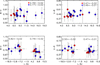 |
Fig. 1 Color indices of the dynamically new comets against their heliocentric distances. Red circles indicate the comets from this study and blue circles denote the dynamically new comets selected from Jewitt (2015). Top Panel: all data points; the mean values calculated for each of subsamples separately are inserted in the figure. Bottom Panel: pre- and post-perihelion observations separately assuming that the two subsamples (“red” and “blue”) belong to the same selection. Error bars of 3σ are shown. |
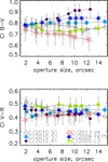 |
Fig. 2 Dependence of the color indices of the bright NICs on angular distance from the photometric center. |
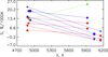 |
Fig. 3 Normalized reflectivity gradients of the selected NICs in the BV and VR spectral regions. Blue and red symbols indicate data points for the comets observed before and after perihelia, respectively; the target with a different spectral behavior is indicated in green. |
4.2 Distant activity
Table 5 gives some photometric parameters characterizing the activity of the observed comets: the R-magnitudes corrected to 0∘ phase angle, corresponding Afρ parameters, dust mass production rates, target heliocentric distances onthe moments of observations, aperture radii expressed inarcsec and km (as projected at the target distances), and the slopes of a log-log fit to the surface brightness profiles. The slope parameters are confined between –0.90 and –1.67, although most of the target profiles weresuccessfully fitted with a slope falling between –1.25 and –1.62. The comae of the two comets had small apparent extension and were too faint to be fitted. In general, the derived slope values are typical for distant active objects, indicating that the comae of the targeted comets are consistent with a steady-state model, which takes into accountthe interaction of outflowing particles with solar radiation pressure (Jewitt & Meech 1987; Lowry & Fitzsimmons 2005).
The comets demonstrated the various levels of physical activity; two of the comets were highly active during the observations with Afρ parameters surpassing 3000 cm, meanwhile the calculated Afρ for three returning comets were less than 260 cm. The lower level of the physical activity of returning comets at large distances from the Sun has been mentioned in the literature and explained as a result of loosing volatiles during previous revolutions and developing a crust mantle on the surfaces (Lowry et al. 1999; Lowry & Fitzsimmons 2001; Mazzotta Epifani et al. 2007; Meech et al. 2009; Mazzotta Epifani et al. 2014; Sárneczky et al. 2016). Eight comets from our sample have been previously characterized with the Afρ (Mazzotta Epifani et al. 2014; Sárneczky et al. 2016). The estimates of the activity from literature for these comets are in reasonable agreement with the Afρ values derived in this work, taking into account the different geometrical circumstances of observations and different reference radii used for the Afρ calculation. We observed distant pre-perihelion activity between 12.7 and 5.7 au for seven comets from our sample. According to Meech et al. (2009), blackbody equilibrium temperatures at these distances correspond to 100–140 K, which are well below the H2 O sublimation temperature. Provided that the onset of activity has probably happened at larger distances, the plausible mechanism initiating the activity of these comets could be annealing of amorphous water ice (see Prialnik et al. (2004) and references therein; Meech et al. 2009).
It has been noted that evolution of the pre-perihelion activity of dynamically new comets is shallow and highly asymmetric respective to a perihelion (A’Hearn et al. 1995; Meech et al. 2009; Rousselot et al. 2014). These features have been explained assuming that halos containing high albedo pure icy grains are formed around the nuclei at large distances from the Sun owing to transient activity (Knight & Schleicher 2015; Bodewits et al. 2015; Paganini et al. 2012). Unfortunately, we do not have enough data to trace individual profiles of the pre-perihelion activity in a wide range of heliocentric distances. Therefore we selected the moderately active comets (Afρ less than 2000 cm) to compare them within a group. The Afρ parameters versus heliocentric distance are depicted in Fig. 4. Three returning comets (denoted with asterisks) demonstrated approximately similar activity levels beforeand after passages through the perihelia. The selected dynamically new comets, which we observed after the perihelion passages, seem to have higher production rates than those observed before the perihelia at approximately the same distances. The trend seems to be opposite from that observed for dynamically new comets with small perihelion distances. For the comets approaching close to the Sun the peak of activity around perihelia is likely caused by the sublimation of halo grains. Vaporizing gradually at small distances from the Sun, these particles contribute significantly to the coma brightness; meanwhile the post perihelion activity is controlled by outgassing from the nucleus and decreases fast with heliocentric distance (A’Hearn et al. 1995). Distant active comets reach perihelia and experience maximal heating at the distances, where halo grains could not have vaporized significantly to cause the profile assymetry. Therefore the possible asymmetry of the activity around perihelia could be due to thermal lag.
Comet C/2010 U3 (Boattini), which was observed at a heliocentric distance of 12.7 au (the largest distance among the investigated targets) on its inbound part of the orbit, has probably represented a different pattern of activity. According to the literature and our yet unpublished observations, the comet has been dimming and becoming more diffuse approaching the Sun as if it had experienced an outburst at a very large heliocentric distance (Jewitt 2015; Sárneczky et al. 2016).
The dust production rates were calculated based on the measured Afρ values and on the input set of parameters discussed in Sect. 3. The dust production rate is a model dependent parameter, therefore there is a disagreement between the values presented here and those published by Mazzotta Epifani et al. (2014) for the same targets. The main reason for the inconsistency is considerably lower outflow velocities: for grains corresponding to the peak of the size distribution (between 40 μm and 90 μm for the various targets) we estimated the outflow velocities to be between 6 and 15 m s−1 against 20 m s−1 used by Mazzotta Epifani et al. (2014).
R magnitudes, Afρ parameters, slopes, and dust production rates for the targeted comets.
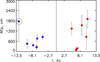 |
Fig. 4 Pre- and post-perihelion Afρ values vs heliocentric distances for the targeted comets exhibiting moderate activity. Filled circles indicate dynamicallynew comets and asterisks indicate returning comets. The circled point indicates comet C/2010 U3 (Boattini) (see explanation in the text). |
5 Summary
We present the broadband photometric data processed uniformly for 14 comets with orbital perihelia located at heliocentric distances at which the sublimation of water ice is negligible. The orbits of 10 comets from our sample are classified as dynamically new, therefore it is expected that the comets have not undergone thermal processing due to residence in the inner part of the solar system. Some of the targeted comets were observed at distances between 12.7 and 5.7 au before the perihelion passages, the others were observed after their perihelia at comparatively similar distances. The main results of the analysis can be summarized as follows:
The investigated comets have demonstrated variable levels of activity parameterized with the Afρ between 95 ± 10 cm and 9600 ± 300 cm. Three returning comets have been less active than dynamically new comets (the Afρ are between 95 ± 10 and 260 ± 40). The lower activity of old comets could be a sequence of losing volatiles and developing the dust mantles on surfaces as a result of previous revolutions (A’Hearn et al. 1995; Mazzotta Epifani et al. 2007). The dust production rates of the comet nuclei were estimated from the Afρ parameters to be between 1–3 kg s−1 and 4–100 kg s−1 for the returning and dynamically new comets.
The post-perihelion activity of the observed dynamically new comets as a group seems to be higher than the activity observed at the similar heliocentric distances pre-perihelion. Taking into account that the sample of the investigated targets are small, we can only arrive at a tentative conclusion that the analysis of activity of the selected dynamically new comets as a group shows possible asymmetry respective to perihelia, which could be caused by thermal lag.
The analysis of color indices revealed that the scattered light by coma particles is redder than the incident solar radiation for all the targets. The mean values of normalized reflectivity gradients within a group amount to 14 ± 2% per 1000 Å and 3 ± 2% per 1000 Å for the BV and VR spectral regions.
The color indices complemented with results taken from Jewitt (2015) indicate that dynamically new comets, which move on their inbound part of orbit beyond the water-ice sublimation zone, have slightly redder comae in the BV spectral region than those comets that have passed through perihelia (mean B − V equals to 0.82 ± 0.02 and 0.74 ± 0.02, respectively). This conclusion should be verified using larger sample of new comets with perihelia at large distances from the Sun.
Acknowledgements
The observations conducted with 2 m Liverpool telescope were supported by the European Community’s Seventh Framework Programme (FP7/2013-2016) under grant agreement number 312430 (OPTICON). The observations at the 6 m BTA telescope were carried out with the financial support of the Ministry of Education and science of the Russian Federation (agreement No. 14.619.21.0004, project ID RFMEEI61914X0004). I. Kulyk acknowledges support through an award from Université Bourgogne Franche-Comté, France. The authors thank the unknown referee for valuable comments, which helped to strengthen the paper.
References
- Afanasiev, V. L., & Moiseev, A. V. 2011, Baltic Astron., 20, 363 [Google Scholar]
- A’Hearn, M. F., Schleicher, D. G., Millis, R. L., Feldman, P. D., & Thompson, D. T. 1984, AJ, 89, 579 [NASA ADS] [CrossRef] [Google Scholar]
- A’Hearn, M. F., Millis, R. C., Schleicher, D. O., Osip, D. J., & Birch, P. V. 1995, Icarus, 118, 223 [NASA ADS] [CrossRef] [Google Scholar]
- A’Hearn, M. F., Feaga, L. M., Keller, H. U., et al. 2012, ApJ, 758, 29 [NASA ADS] [CrossRef] [Google Scholar]
- Arvesen, J. C., Griffin, Jr. R. N., & Pearson, Jr., B. D. 1969, Appl. Opt., 8, 2215 [NASA ADS] [CrossRef] [Google Scholar]
- Bar-Nun, A., Herman, G., Laufer, D., & Rappaport, M. L. 1985, Icarus, 63, 317 [CrossRef] [Google Scholar]
- Bentley, M. S., Schmied, R., Mannel, T., et al. 2016, Nature, 537, 73 [NASA ADS] [CrossRef] [Google Scholar]
- Bessell, M. S. 1999, PASP, 111, 1426 [NASA ADS] [CrossRef] [Google Scholar]
- Bodewits, D., Kelley, M. S. P., Li, J.-Y., Farnham, T. L., & A’Hearn, M. F. 2015, ApJ, 802, L6 [NASA ADS] [CrossRef] [Google Scholar]
- Cochran, A. L., Barker, E. S., & Gray, C. L. 2012, Icarus, 218, 144 [NASA ADS] [CrossRef] [Google Scholar]
- Cochran, A. L., Levasseur-Regourd, A.-C., Cordiner, M., et al. 2015, Space Sci. Rev., 197, 9 [NASA ADS] [CrossRef] [Google Scholar]
- de Freitas Pacheco, J. A., Singh, P. D., & Landaberry, S. J. C. 1988, MNRAS, 235, 457 [NASA ADS] [CrossRef] [Google Scholar]
- Della Corte, V., Rotundi, A., Fulle, M., et al. 2015, A&A, 583, A13 [NASA ADS] [CrossRef] [EDP Sciences] [Google Scholar]
- Dello Russo, N., Kawakita, H., Vervack, R. J., & Weaver, H. A. 2016, Icarus, 278, 301 [NASA ADS] [CrossRef] [Google Scholar]
- Disanti, M. A., & Mumma, M. J. 2008, Space Sci. Rev., 138, 127 [NASA ADS] [CrossRef] [Google Scholar]
- Dlugach, J., Ivanova, O., Mishchenko, M., & Afanasiev, V. L. 2018, J. Quant. Spec. Radiat. Transf., 205, 80 [Google Scholar]
- Dones, L., Weissman, P. R., Levison, H. F., & Duncan, M. J. 2004, in Oort Cloud Formation and Dynamics, eds. M. C. Festou, H. U. Keller, & H. A., Weaver, ASP Conf. Ser., 323, 371 [Google Scholar]
- Duncan, M., Quinn, T., & Tremaine, S. 1987, AJ, 94, 1330 [NASA ADS] [CrossRef] [Google Scholar]
- Duncan, M. J., & Levison, H. F. 1997, Science, 276, 1670 [NASA ADS] [CrossRef] [PubMed] [Google Scholar]
- Emel’yanenko, V. V., Asher, D. J., & Bailey, M. E. 2004, MNRAS, 350, 161 [NASA ADS] [CrossRef] [Google Scholar]
- Fink, U. 2009, Icarus, 201, 311 [Google Scholar]
- Fukugita, M., Ichikawa, T., Gunn, J. E., et al. 1996, AJ, 111, 1748 [NASA ADS] [CrossRef] [Google Scholar]
- Fulle, M. 1994, A&A, 282, 980 [NASA ADS] [Google Scholar]
- Fulle, M., Levasseur-Regourd, A. C., McBride, N., & Hadamcik, E. 2000, AJ, 119, 1968 [Google Scholar]
- Fulle, M., Della Corte, V., Rotundi, A., et al. 2015, ApJ, 802, 12 [Google Scholar]
- Gomes, R. S., Fernandez, J. A., Gallardo, T., & Brunini, A. 2008, in The Solar System Beyond Neptune, eds. M. A. Barucci, H. Boehnhardt, D. P. Cruikshank, & A. Morbidelli (Tucson: University of Arizona Press), 259 [Google Scholar]
- Guilbert-Lepoutre, A., Besse, S., Mousis, O., et al. 2015, Space Sci. Rev., 197, 271 [NASA ADS] [CrossRef] [Google Scholar]
- Hanner, M. 1983a, Naturwissenschaften, 70, 581 [NASA ADS] [CrossRef] [Google Scholar]
- Hanner, M. S. 1983b, in Cometary Exploration, ed. T. I. Gombosi, 2, 1 [Google Scholar]
- Heisler, J., & Tremaine, S. 1986, Icarus, 65, 13 [NASA ADS] [CrossRef] [Google Scholar]
- Holmberg, J., Flynn, C., & Portinari, L. 2006, MNRAS, 367, 449 [NASA ADS] [CrossRef] [Google Scholar]
- Ivanova, O., Neslušan, L., Krišandová, Z. S., et al. 2015, Icarus, 258, 28 [NASA ADS] [CrossRef] [Google Scholar]
- Jenniskens, P., & Blake, D. F. 1994, Science, 265, 753 [NASA ADS] [CrossRef] [Google Scholar]
- Jewitt, D. 2009, AJ, 137, 4296 [NASA ADS] [CrossRef] [Google Scholar]
- Jewitt, D. 2015, AJ, 150, 201 [NASA ADS] [CrossRef] [Google Scholar]
- Jewitt, D. C. 2002, AJ, 123, 1039 [NASA ADS] [CrossRef] [Google Scholar]
- Jewitt, D. C., & Meech, K. J. 1986, in ESLAB Symposium on the Exploration of Halley’s Comet, eds. B. Battrick, E. J. Rolfe, & R. Reinhard, ESA SP, 250 [Google Scholar]
- Jewitt, D. C., & Meech, K. J. 1987, ApJ, 317, 992 [NASA ADS] [CrossRef] [Google Scholar]
- Kelley, M. S., Reach, W. T., & Lien, D. J. 2008, Icarus, 193, 572 [NASA ADS] [CrossRef] [Google Scholar]
- Knight, M. M., & Schleicher, D. G. 2015, AJ, 149, 19 [NASA ADS] [CrossRef] [Google Scholar]
- Korsun, P. P. 2005, Kinematika i Fizika Nebesnykh Tel Supplement, 5, 465 [NASA ADS] [Google Scholar]
- Korsun, P. P., & Chörny, G. F. 2003, A&A, 410, 1029 [NASA ADS] [CrossRef] [EDP Sciences] [Google Scholar]
- Korsun, P. P., Kulyk, I. V., Ivanova, O. V., et al. 2010, Icarus, 210, 916 [NASA ADS] [CrossRef] [Google Scholar]
- Korsun, P. P., Rousselot, P., Kulyk, I. V., Afanasiev, V. L., & Ivanova, O. V. 2014, Icarus, 232, 88 [NASA ADS] [CrossRef] [Google Scholar]
- Lamy, P. L., Toth, I., Weaver, H. A., A’Hearn, M. F., & Jorda, L. 2009, A&A, 508, 1045 [NASA ADS] [CrossRef] [EDP Sciences] [Google Scholar]
- Landolt, A. U. 1992, AJ, 104, 340 [NASA ADS] [CrossRef] [Google Scholar]
- Lasue, J., Levasseur-Regourd, A. C., Hadamcik, E., & Alcouffe, G. 2009, Icarus, 199, 129 [NASA ADS] [CrossRef] [Google Scholar]
- Levison, H. F. 1996, in Completing the Inventory of the Solar System, eds. T. Rettig, & J. M. Hahn, ASP Conf. Ser., 107173 [Google Scholar]
- Levison, H. F., Morbidelli, A., Dones, L., et al. 2002, Science, 296, 2212 [NASA ADS] [CrossRef] [Google Scholar]
- Levison, H. F., Morbidelli, A., Van Laerhoven, C., Gomes, R., & Tsiganis, K. 2008, Icarus, 196, 258 [NASA ADS] [CrossRef] [Google Scholar]
- Lowry, S. C., & Fitzsimmons, A. 2001, A&A, 365, 204 [NASA ADS] [CrossRef] [EDP Sciences] [Google Scholar]
- Lowry, S. C., & Fitzsimmons, A. 2005, MNRAS, 358, 641 [NASA ADS] [CrossRef] [Google Scholar]
- Lowry, S. C., Fitzsimmons, A., Cartwright, I. M., & Williams, I. P. 1999, A&A, 349, 649 [NASA ADS] [Google Scholar]
- Lowry, S., Fitzsimmons, A., Lamy, P., & Weissman, P. 2008, in The Solar System Beyond Neptune, eds. M. A. Barucci, H. Boehnhardt, D. P. Cruikshank, & A. Morbidelli (Tucson: University of Arizona Press), 397 [Google Scholar]
- Mandt, K. E., Mousis, O., Marty, B., et al. 2015, Space Sci. Rev., 197, 297 [NASA ADS] [CrossRef] [Google Scholar]
- Mazzotta Epifani, E., Palumbo, P., Capria, M. T., et al. 2007, MNRAS, 381, 713 [NASA ADS] [CrossRef] [Google Scholar]
- Mazzotta Epifani, E., Palumbo, P., Capria, M. T., et al. 2009, A&A, 502, 355 [NASA ADS] [CrossRef] [EDP Sciences] [Google Scholar]
- Mazzotta Epifani, E., Perna, D., Di Fabrizio, L., et al. 2014, A&A, 561, A6 [NASA ADS] [CrossRef] [EDP Sciences] [Google Scholar]
- Meech, K. J., & Jewitt, D. C. 1987, A&A, 187, 585 [NASA ADS] [Google Scholar]
- Meech, K. J., & Svoren, J. 2004, in Comets II, eds. M. C. Festou, H. U. Keller, & H. A. Weaver (Tucson: University of Arizona Press), 317 [Google Scholar]
- Meech, K. J., Pittichová, J., Bar-Nun, A., et al. 2009, Icarus, 201, 719 [NASA ADS] [CrossRef] [Google Scholar]
- Meech, K. J., Schambeau, C. A., Sorli, K., et al. 2017, AJ, 153, 206 [NASA ADS] [CrossRef] [Google Scholar]
- Merline, W. J., & Howell, S. B. 1995, Exp. Astron., 6, 163 [NASA ADS] [CrossRef] [Google Scholar]
- Morbidelli, A., Levison, H. F., & Gomes, R. 2008, in The Solar System Beyond Neptune, eds. M. A. Barucci, H. Boehnhardt, D. P. Cruikshank,& A. Morbidelli (Tucson: University of Arizona Press), 275 [Google Scholar]
- Moreno, F., Snodgrass, C., Hainaut, O., et al. 2016, A&A, 587, A155 [NASA ADS] [CrossRef] [EDP Sciences] [Google Scholar]
- Mukai, T., Ishimoto, H., Kozasa, T., Blum, J., & Greenberg, J. M. 1992, A&A, 262, 315 [NASA ADS] [Google Scholar]
- Newburn, R. L., & Spinrad, H. 1985, AJ, 90, 2591 [NASA ADS] [CrossRef] [Google Scholar]
- Newburn, R. L., Bell, J. F., & McCord, T. B. 1981, AJ, 86, 469 [NASA ADS] [CrossRef] [Google Scholar]
- Niimi, R., Kadono, T., Tsuchiyama, A., et al. 2012, ApJ, 744, 18 [NASA ADS] [CrossRef] [Google Scholar]
- Oke, J. B. 1990, AJ, 99, 1621 [NASA ADS] [CrossRef] [Google Scholar]
- Paganini, L., Mumma, M. J., Villanueva, G. L., et al. 2012, ApJ, 748, 13 [NASA ADS] [CrossRef] [Google Scholar]
- Prialnik, D., Benkhoff, J., & Podolak, M. 2004, in Comets II, eds. M. C. Festou, H. U. Keller, & H. A. Weaver (Tucson: University of Arizona Press), 359–387 [Google Scholar]
- Rotundi, A., Sierks, H., Della Corte, V., et al. 2015, Science, 347, aaa3905 [NASA ADS] [CrossRef] [Google Scholar]
- Rousselot, P., Korsun, P. P., Kulyk, I. V., et al. 2014, A&A, 571, A73 [NASA ADS] [CrossRef] [EDP Sciences] [Google Scholar]
- Sárneczky, K., Szabó, G. M., Csák, B., et al. 2016, AJ, 152, 220 [NASA ADS] [CrossRef] [Google Scholar]
- Sekanina, Z., Larson, S. M., Hainaut, O., Smette, A., & West, R. M. 1992, A&A, 263, 367 [NASA ADS] [Google Scholar]
- Singh, P. D., de Almeida, A. A., & Huebner, W. F. 1992, AJ, 104, 848 [NASA ADS] [CrossRef] [Google Scholar]
- Snodgrass, C., Jehin, E., Manfroid, J., et al. 2016, A&A, 588, A80 [NASA ADS] [CrossRef] [EDP Sciences] [Google Scholar]
- Solontoi, M., Ivezić, Ž., Jurić, M., et al. 2012, Icarus, 218, 571 [NASA ADS] [CrossRef] [Google Scholar]
- Stetson, P. B. 1987, PASP, 99, 191 [NASA ADS] [CrossRef] [Google Scholar]
- Storrs, A. D., Cochran, A. L., & Barker, E. S. 1992, Icarus, 98, 163 [NASA ADS] [CrossRef] [Google Scholar]
- Wada, K., Tanaka, H., Suyama, T., Kimura, H., & Yamamoto, T. 2008, ApJ, 677, 1296 [NASA ADS] [CrossRef] [Google Scholar]
- Weiler, M., Rauer, H., Knollenberg, J., Jorda, L., & Helbert, J. 2003, A&A, 403, 313 [NASA ADS] [CrossRef] [EDP Sciences] [Google Scholar]
- Willacy, K., Alexander, C., Ali-Dib, M., et al. 2015, Space Sci. Rev., 197, 151 [NASA ADS] [CrossRef] [Google Scholar]
- Womack, M., Festou, M. C., & Stern, S. A. 1997, AJ, 114, 2789 [NASA ADS] [CrossRef] [Google Scholar]
- Womack, M., Sarid, G., & Wierzchos, K. 2017, PASP, 129, 031001 [NASA ADS] [CrossRef] [Google Scholar]
All Tables
R magnitudes, Afρ parameters, slopes, and dust production rates for the targeted comets.
All Figures
|
Fig. 1 Color indices of the dynamically new comets against their heliocentric distances. Red circles indicate the comets from this study and blue circles denote the dynamically new comets selected from Jewitt (2015). Top Panel: all data points; the mean values calculated for each of subsamples separately are inserted in the figure. Bottom Panel: pre- and post-perihelion observations separately assuming that the two subsamples (“red” and “blue”) belong to the same selection. Error bars of 3σ are shown. |
| In the text | |
|
Fig. 2 Dependence of the color indices of the bright NICs on angular distance from the photometric center. |
| In the text | |
|
Fig. 3 Normalized reflectivity gradients of the selected NICs in the BV and VR spectral regions. Blue and red symbols indicate data points for the comets observed before and after perihelia, respectively; the target with a different spectral behavior is indicated in green. |
| In the text | |
|
Fig. 4 Pre- and post-perihelion Afρ values vs heliocentric distances for the targeted comets exhibiting moderate activity. Filled circles indicate dynamicallynew comets and asterisks indicate returning comets. The circled point indicates comet C/2010 U3 (Boattini) (see explanation in the text). |
| In the text | |
Current usage metrics show cumulative count of Article Views (full-text article views including HTML views, PDF and ePub downloads, according to the available data) and Abstracts Views on Vision4Press platform.
Data correspond to usage on the plateform after 2015. The current usage metrics is available 48-96 hours after online publication and is updated daily on week days.
Initial download of the metrics may take a while.