| Issue |
A&A
Volume 610, February 2018
|
|
|---|---|---|
| Article Number | L10 | |
| Number of page(s) | 4 | |
| Section | Letters to the Editor | |
| DOI | https://doi.org/10.1051/0004-6361/201732402 | |
| Published online | 22 February 2018 | |
Letter to the Editor
A magnetar model for the hydrogen-rich super-luminous supernova iPTF14hls
Unidad Mixta Internacional Franco-Chilena de Astronomía (CNRS, UMI 3386), Departamento de Astronomía, Universidad de Chile,
Camino El Observatorio 1515,
Las Condes,
Santiago, Chile
e-mail: This email address is being protected from spambots. You need JavaScript enabled to view it.
Received:
2
December
2017
Accepted:
14
January
2018
Abstract
Transient surveys have recently revealed the existence of H-rich super-luminous supernovae (SLSN; e.g., iPTF14hls, OGLE-SN14-073) that are characterized by an exceptionally high time-integrated bolometric luminosity, a sustained blue optical color, and Doppler-broadened H I lines at all times. Here, I investigate the effect that a magnetar (with an initial rotational energy of 4 × 1050 erg and field strength of 7 × 10¹³ G) would have on the properties of a typical Type II supernova (SN) ejecta (mass of 13.35 M⊙, kinetic energy of 1.32 × 1051 erg, 0.077 M⊙ of 56Ni) produced by the terminal explosion of an H-rich blue supergiant star. I present a non-local thermodynamic equilibrium time-dependent radiative transfer simulation of the resulting photometric and spectroscopic evolution from 1 d until 600 d after explosion. With the magnetar power, the model luminosity and brightness are enhanced, the ejecta is hotter and more ionized everywhere, and the spectrum formation region is much more extended. This magnetar-powered SN ejecta reproduces most of the observed properties of SLSN iPTF14hls, including the sustained brightness of −18 mag in the R band, the blue optical color, and the broad H I lines for 600 d. The non-extreme magnetar properties, combined with the standard Type II SN ejecta properties, offer an interesting alternative to the pair-unstable super-massive star model recently proposed, which involves a highly energetic and super-massive ejecta. Hence, such Type II SLSNe may differ from standard Type II SNe exclusively through the influence of a magnetar.
Key words: radiative transfer / hydrodynamics / supernovae: general / stars: magnetars
© ESO 2018
1 Introduction
Super-luminous supernovae (SLSNe) owe their exceptional instantaneous and/or time-integrated luminosities to a non-standard source of energy and power. This power source may be interaction between a (standard-energy) ejecta with dense, massive, and slow-moving circumstellar material, leading to an interacting supernova (SN), generally of Type IIn (H-rich; Schlegel 1990; Chugai 2001, 2016; Smith et al. 2007; Moriya et al. 2011; Fransson et al. 2014; Dessart et al. 2015, 2016). The spectral signatures are unambiguous, with the presence of electron-scattering broadened, rather than Doppler-broadened, emission lines. Alternatively, this power source may be a greater-than-standard production of unstable isotopes, and in particular 56Ni, asin pair-instability SNe from super-massive stars (Barkat et al. 1967). The high metal content of these ejecta produces strongly blanketed, red spectra with small/moderate line widths at and beyond maximum (Dessart et al. 2013b). The final alternative is energy injection from a compact remnant, as in a strongly magnetized neutron star with a fast initial spin. For moderate magnetic field strengths and initial spin periods, the spin-down timescale may be equal to or greater than the expansion timescale of the ejecta, allowing a powerful heating on day/week timescales (Kasen & Bildsten 2010). This engine is believed to be at the origin of most, and perhaps all, SLSN Ic, which are characterized by relatively short rise times, blue colors at all times, and the dominance of spectral lines from intermediate-mass elements such as oxygen (Quimby et al. 2011; Dessart et al. 2012b; Nicholl et al. 2013; Greiner et al. 2015; Mazzali et al. 2016; Chen et al. 2017). Because of the nature of these processes, SLSNe are generally thought to be connected to core-collapse SNe.
Arcavi et al. (2017, hereafter A17) recently reported the unique properties of the Type II SLSN iPTF14hls. This event has an inferred R-band absolute magnitude of −18 mag for about 600 d (inferred time-integrated bolometric luminosity of 2.2 × 1050 erg), with fluctuations of amplitude 0.5 mag. Its color is blue throughout these 2 yr, with V − I ~ 0.2 mag. The optical spectra of SLSN iPTF14hls evolve little from about 100 to 600 d after the inferred (but uncertain) time of explosion. Hα, which is the strongest line in the spectrum, evolves little in strength (relative to the adjacent continuum) and in width. A17 inferred an Hα formation region that is much more extended than the radius of continuum formation, and proposed that this external region corresponds to a massive shell ejected a few hundred days before a terminal explosion. In this context, iPTF14hls would be associated with a pair-unstable super-massive star.
In this configuration, the inner ejecta from a terminal explosion would ram into a massive (e.g., 50 M⊙) energetic (e.g., 1052 erg) outer shell with a mean mass-weighted velocity of ~4000 km s−1 and located at 1015–1016 cm. Electron-scattering broadened narrow lines do not form since photons from the shock are reprocessed in a fast outer shell in homologous expansion. This model is the high-energy counterpart to the proposed model for SN 1994W analogs (Chugai 2016; Dessart et al. 2016). The interaction leads to the formation of a heat wave that propagates outward in the outer shell, causing reionization, and shifting the photosphere to large radii (or high velocities). After a bolometric maximum is reached on a diffusion timescale, the outer shell recombines and the photosphere recedes in mass/velocity space. Compared to interaction with a slow long-lived dense wind, the interaction with a massive energetic explosively ejected outer shell (steep density fall-off, homologous velocity) is expected to be stronger early on and weaken faster with time. Surprisingly, iPTF14hls shows a very slow evolving brightness and color, broad lines (FWHM of ~10 000 km s−1), and no sign of recombination out to 600 d.
In this Letter, I show how a magnetar-powered model combined with a standard-energy explosion of a 15 M⊙ supergiant star can reproduce most of the properties of iPTF14hls. In the next section, I discuss the numerical approach, including the treatment of the magnetar power in the non-local thermodynamic equilibrium (non-LTE) time-dependent radiative transfer code cmfgen (Hillier & Dessart 2012). In Sect. 3, I present the results for this magnetar-powered model and compare it with results previously published for a standard SN II-P (model m15mlt3; Dessart et al. 2013a) and a pair-instability Type II SN (model R190NL; Dessart et al. 2013b), which I then compare with the photometric and spectroscopic observations of iPTF14hls. Following A17, I adopt an explosion date MJD = 56 922.53, a distance of 156 Mpc, a redshift of 0.0344, and I assume zero reddening. Section 4 concludes the Letter.
2 Numerical approach
The magnetar-powered SN model (named a4pm1) stems from a progenitor star of initially 15 M⊙ that was evolved with mesa (Paxton et al. 2015) at a metallicity of 10−7 . This model, which reached core collapse as a blue supergiant star, was exploded with v1d (Livne 1993; Dessart et al. 2010a,b) to yield an ejecta of 13.35 M⊙, an explosion energy of 1.32 × 1051 erg, and a 56Ni mass of 0.077 M⊙. Model a4pm1 has a similar He core mass and chemical stratification as model m15mlt3 from Dessart et al. (2013a). Hydrogen dominates the ejecta composition with 7.53 M⊙. I adopted strong chemical mixing (this explosion model will be used later for a study of SN 1987A; Dessart et al., in prep.). Hence, the original low-metallicity of the envelope was erased by the mixing of the metal-rich core material with the metal-poor progenitor envelope. At 1 d, this model was remapped into cmfgen (Hillier & Dessart 2012) and followed until 600 d using the standard procedure (Dessart et al. 2013a).
The central feature of model a4pm1 is that starting at day one, I injected a magnetar power given by
 where Epm, Bpm , Rpm , Ipm , and ωpm are the initial rotational energy, magnetic field, radius, moment of inertia, and angular velocity of the magnetar; c is the speed of light. I used Epm = 4 × 1050 erg, Bpm = 7 × 10¹³ G, Ipm = 1045 g cm2, and Rpm = 106 cm (see Kasen & Bildsten 2010 for details). This magnetar has a spin-down timescale of 478 d. The energy released during the first day, which was neglected, is only 0.2% of the total magnetar energy. Furthermore, I assumed that all the energy liberated by the magnetar is channelled into ejecta internal energy (and eventually radiation); cmfgen does not treat dynamics. This is a good approximation for this weakly magnetized object (see also Dessart & Audit 2018). In cmfgen, I treated the magnetar power in the same way as radioactive decay. Energy was injected as 1 keV electrons for which the degradation spectrum was computed. The contribution to heat and non-thermal excitation/ionization was then calculated explicitly.
To mimic the effect of fluid instabilities (Chen et al. 2016; Suzuki & Maeda 2017), the magnetar energy was deposited over a range of ejecta velocities. The deposition profile follows ρ for V < V0, and ρ exp (−[(V − V0)/dV]2) for V > V0. Model a4pm1 used V0 = 4000 km s−1 and d V = 2000 km s−1. A normalization was applied so that the volume integral of this deposition profile yielded the instantaneous magnetar power at that time. With this choice, the energy deposition profile influences the model luminosity most strongly before maximum (Dessart & Audit 2018).
I compare the results to the SN II-P model m15mlt3 (Dessart et al. 2013a) and the pair-instability Type II SN model R190NL (Dessart et al. 2013b). The model properties are given in Table 1.
Summary of the model properties.
3 Results
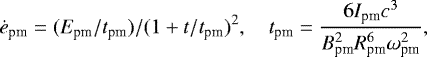
The top panel of Fig. 1 shows the bolometric light curves for the model set. The magnetar-powered SN is super-luminous, intermediate during the first year between the standard SN II-P model m15mlt3 and the PISN model R190NL. It is the brightest of all three at late times. Model a4pm1 is faint early on because of the small progenitor radius. After ~50 d, it closely follows the iPTF14hls R-band light curve (bottom panel of Fig. 1). The adopted magnetar power is continuous and monotonic, therefore it cannot explain the observed R-band fluctuations of ~0.5 mag in iPTF14hls. These might indicate the intrinsic variability of the proto-magnetar. However, the rotation energy of 4 × 1050 erg and the magnetic strength of 7 × 10¹³ G in model a4pm1 yield a suitable match to the overall brightness and slow fading. The discrepancy at early times would be reduced if an extended progenitor were used. A broader energy deposition profile or asymmetry might resolve this discrepancy.
Figure 2 shows that over the time span 100–600 d after explosion, model a4pm1 has a weakly evolving and blue optical color, in contrast to the non-monotonic and strongly varying color evolution of models m15mlt3 and R190NL. Up to ~50 d, model a4pm1 is redder because the progenitor is compact rather than extended. This additional cooling from expansion is superseded after ~ 50 d by the slowly decreasing magnetar power. Model a4pm1 closely follows the V − I color of iPTF14hls, which is fixed at about 0.2 mag (A17).
Up to the time of maximum, this bolometric and color evolution reflects the evolution of the ejecta properties and of the photosphere, taken as the location where the inward-integrated electron scattering optical depth τes equals 2/3 (Fig. 3). In model a4pm1, the initial evolution is very rapid, as obtained in models of blue supergiant star explosions and inferred from the observationsof SN 1987A (Dessart & Hillier 2010). At the photosphere, the velocity (temperature) drops from 17 300 km s−1 (14 000 K) at 1.2 d down to 7500 km s−1 (5600 K) at 10 d. After 10 d, photospheric cooling is inhibited and even reversed by magnetar heating, and the model evolves at a near constant photospheric temperature of ~7000 K out to 600 d. Magnetar heating prevents the recombination of the ejecta material, so that hydrogen remains partially ionized at all times. This allows the photosphere of model a4pm1 to recede slowly in mass/velocity space and to reach radii > 1016 cm, greater thanin a standard Type II SN (Dessart & Hillier 2011) and comparable to model R190NL (Dessart et al. 2013b).
In a standard Type II SN, the photosphere follows the layer at the interface between neutral and ionized material (which essentially tracks the H I recombination front). Recombination speeds up the recession of the photosphere and makes the ejecta optically thin on a shorter timescale (typically of ~ 100 d) than in the case of constant ionization. This process is mitigated by the ionization freeze-out in Type II SN ejecta (Utrobin & Chugai 2005; Dessart & Hillier 2008). In model a4pm1, the electron scattering optical depth τes drops from 1.21 × 10⁶ at 1.21 d to 1.33 at 600 d, which is close to the value of 4.92 that would result for constant ionization (τes ∝ 1∕t2). This means that in model a4pm1, the inhibition of recombination maintains the ejecta in an optically thick state to electron scattering for more than 600 d. Lines of H I or Ca II will remain optically thick (and therefore broad) for even longer. Between 75% and 100% of the magnetar power goes into heat. Whatever remains is shared equally between excitation and ionization. In model a4pm1, non-thermaleffects are inhibited by the partial ejecta ionization.
The photospheric evolution is not a reliable guide to understand the SN luminosity after maximum. The large photospheric radii combined with the large ejecta ionization cause a flux dilution by electron scattering. The SN spectrum may resemble a blackbody (A17), but at best diluted, with a thermalization radius much smaller than the photospheric radius (Eastman et al. 1996; Dessart & Hillier 2005). For example, at 250 d, τes is 7.4, which is too small to ensure thermalization. Instead, the conditions are nebular and the SN luminosity equals the magnetar power (Fig. 1).
Model a4pm1 shows very little spectral evolution from 104 d (date of the first spectrum taken for iPTF14hls) until 600 d (Fig. 4), which in part reflects the fixed photospheric conditions (velocity and temperature) after 10 d (Fig. 3). The spectra show the H i Balmer lines, Fe II lines around 5000 Å, and the Ca II triplet around 8500 Å. After about 300 d, the triplet is seen only in emission. Hα stays broad at all times, and the Ca II doublet 7300 Å strengthens as the conditions in the ejecta become more nebular. Throughout this evolution, there is little sign of the blanketing that would appear in the optical range if the ejecta ionization dropped. The spectral evolution of model a4pm1 is similar to that observed for SLSN iPTF14hls, with a few discrepancies. The model underestimates the width of the Hα absorption trough, although it matches the emission width at all times. Adopting a broader energy-deposition profile would produce broader line absorptions (in a similar way to adopting a stronger 56Ni mixing in Type Ibc SNe; Dessart et al. 2012a).
The model also underestimates the strength of the Ca II emission at late times. The feature at 5900 Å is not predicted by the model. This is probably Na i D, because if it were He i 5875 Å, one would expect a few other optical He i lines, which are not seen. Hence, our model may overestimate the ionization. Allowing for clumping might solve this issue (Jerkstrand et al. 2017).
The Doppler velocity at maximum absorption in H I or Fe II lines is high, greater than the photospheric velocity, and does not change much after about 50 d – the fast outer ejecta material is scanned at early times, before the magnetar has influenced the photosphere (Fig. 5). These lines eventually form over a large volume that extends far above the photosphere. These properties hold qualitatively even in standard Type II SNe.
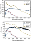 |
Fig. 1 Top: bolometric light curve for models a4pm1 (the dashed line gives the instantaneous magnetar power), m15mlt3 (standard SN II-P), and R190NL (pair-instability SN). Bottom: same as the top, but showing the absolute R-band magnitude. I also add the observations of iPTF14hls corrected for distance and time dilation. The thin blue line in both panels corresponds to model a4pm1 without magnetar power. |
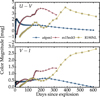 |
Fig. 2 Same as for the top of Fig. 1, but now showing the color magnitude U − V (top) and V − I (bottom). |
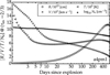 |
Fig. 3 Evolution of photospheric properties in model a4pm1. The x-axis uses a logarithmic scale. |
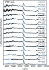 |
Fig. 4 Comparison of the multi-epoch spectra of SLSN iPTF14hls with model a4pm1. Times and wavelengths are given in the rest frame. Model and observations are renormalized at 6800 Å. For each date, I give the R-band magnitude offset (see also Fig. 1). |
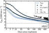 |
Fig. 5 Evolution of the Doppler velocity at maximum absorption in various lines and the photospheric velocity in model a4pm1. I overplot the corresponding values for Hα in iPTF14hls. The x-axis uses a logarithmic scale. The horizontal line gives the ejecta velocity |

4 Conclusion
In this Letter, I have presented the first non-LTE time-dependent radiative transfer simulation of a Type II SN influenced by a magnetar. I have shown that a magnetar-powered SN ejecta from a 1.32 × 1051 erg explosion of a 15 M⊙ supergiant star reproduces most of the observed properties of SLSN iPTF14hls. The modest magnetar properties (Epm = 4 × 1050 erg, Bpm = 7 × 10¹³ G), combined with the standard Type II SN ejecta properties offer an interesting alternative to the pair-unstable super-massive star model of A17, which involves a highly energetic and super-massive ejecta. As discussed in Dessart & Audit (2018), a similar magnetar-powered SN, with a standard ejecta mass and energy, may be at the origin of the SLSN OGLE-SN14-073, for which Terreran et al. (2017) also invoked a highly energetic and super-massive ejecta.
Hence, Type II SLSNe that at all times show a blue color, broad H I spectral lines, and a weaker-than-average blanketing may differ from standard Type II SNe primarily through the influence of a magnetar.
Acknowledgments
I thank Roni Waldman for providing the progenitor used for model a4pm1. This work used computing resources of the mesocentre SIGAMM, hosted by the Observatoire de la Côte d’Azur, France. This research was supported by the Munich Institute for Astro- and Particle Physics (MIAPP) of the DFG cluster of excellence “Origin and Structure of the Universe”.
References
- Arcavi, I., Howell, D. A., Kasen, D., et al. 2017, Nature, 551, 210 [NASA ADS] [CrossRef] [Google Scholar]
- Barkat, Z., Rakavy, G., & Sack, N. 1967, Phys. Rev. Lett., 18, 379 [NASA ADS] [CrossRef] [Google Scholar]
- Chen, K.-J., Woosley, S. E., & Sukhbold, T. 2016, ApJ, 832, 73 [NASA ADS] [CrossRef] [Google Scholar]
- Chen, K.-J., Moriya, T. J., Woosley, S., et al. 2017, ApJ, 839, 85 [NASA ADS] [CrossRef] [Google Scholar]
- Chugai, N. N. 2001, MNRAS, 326, 1448 [NASA ADS] [CrossRef] [Google Scholar]
- Chugai, N. N. 2016, Astron. Lett., 42, 82 [NASA ADS] [CrossRef] [Google Scholar]
- Dessart, L., & Audit, E. 2018, A&A, in press, DOI:10.1051/0004-6361/201732229 [Google Scholar]
- Dessart L., & Hillier, D. J. 2005, A&A, 439, 671 [NASA ADS] [CrossRef] [EDP Sciences] [Google Scholar]
- Dessart, L., & Hillier, D. J. 2008, MNRAS, 383, 57 [NASA ADS] [CrossRef] [Google Scholar]
- Dessart, L., & Hillier, D. J. 2010, MNRAS, 405, 2141 [Google Scholar]
- Dessart, L., & Hillier, D. J. 2011, MNRAS, 410, 1739 [Google Scholar]
- Dessart, L., Livne, E., & Waldman, R. 2010a, MNRAS, 408, 827 [NASA ADS] [CrossRef] [Google Scholar]
- Dessart, L., Livne, E., & Waldman, R. 2010b, MNRAS, 405, 2113 [Google Scholar]
- Dessart, L., Hillier, D. J., Li, C., & Woosley, S. 2012a, MNRAS, 424, 2139 [NASA ADS] [CrossRef] [Google Scholar]
- Dessart, L., Hillier, D. J., Waldman, R., Livne, E., & Blondin, S. 2012b, MNRAS, 426, L76 [NASA ADS] [CrossRef] [Google Scholar]
- Dessart, L., Hillier, D. J., Waldman, R., & Livne, E. 2013a, MNRAS, 433, 1745 [NASA ADS] [CrossRef] [Google Scholar]
- Dessart, L., Waldman, R., Livne, E., Hillier, D. J., & Blondin, S. 2013b, MNRAS, 428, 3227 [NASA ADS] [CrossRef] [Google Scholar]
- Dessart, L., Audit, E., & Hillier, D. J. 2015, MNRAS, 449, 4304 [NASA ADS] [CrossRef] [Google Scholar]
- Dessart, L., Hillier, D. J., Audit, E., Livne, E., & Waldman, R. 2016, MNRAS, 458, 2094 [NASA ADS] [CrossRef] [Google Scholar]
- Eastman, R. G., Schmidt, B. P., & Kirshner, R. 1996, ApJ, 466, 911 [NASA ADS] [CrossRef] [Google Scholar]
- Fransson, C., Ergon, M., Challis, P. J., et al. 2014, ApJ, 797, 118 [NASA ADS] [CrossRef] [Google Scholar]
- Greiner, J., Mazzali, P. A., Kann, D. A., et al. 2015, Nature, 523, 189 [NASA ADS] [CrossRef] [Google Scholar]
- Hillier, D. J., & Dessart, L. 2012, MNRAS, 424, 252 [NASA ADS] [CrossRef] [Google Scholar]
- Jerkstrand, A., Smartt, S. J., Inserra, C., et al. 2017, ApJ, 835, 13 [NASA ADS] [CrossRef] [Google Scholar]
- Kasen, D., & Bildsten, L. 2010, ApJ, 717, 245 [NASA ADS] [CrossRef] [Google Scholar]
- Livne, E. 1993, ApJ, 412, 634 [NASA ADS] [CrossRef] [Google Scholar]
- Mazzali, P. A., Sullivan, M., Pian, E., Greiner, J., & Kann, D. A. 2016, MNRAS, 458, 3455 [NASA ADS] [CrossRef] [Google Scholar]
- Moriya, T., Tominaga, N., Blinnikov, S. I., Baklanov, P. V., & Sorokina, E. I. 2011, MNRAS, 415, 199 [NASA ADS] [CrossRef] [Google Scholar]
- Nicholl, M., Smartt, S. J., Jerkstrand, A., et al. 2013, Nature, 502, 346 [NASA ADS] [CrossRef] [Google Scholar]
- Paxton, B., Marchant, P., Schwab, J., et al. 2015, ApJS, 220, 15 [Google Scholar]
- Quimby, R. M., Kulkarni, S. R., Kasliwal, M. M., et al. 2011, Nature, 474, 487 [NASA ADS] [CrossRef] [Google Scholar]
- Schlegel, E. M. 1990, MNRAS, 244, 269 [Google Scholar]
- Smith, N., Li, W., Foley, R. J., et al. 2007, ApJ, 666, 1116 [NASA ADS] [CrossRef] [Google Scholar]
- Suzuki, A., & Maeda, K. 2017, MNRAS, 466, 2633 [NASA ADS] [CrossRef] [Google Scholar]
- Terreran, G., Pumo, M. L., Chen, T.-W., et al. 2017, Nat. Astron., 1, 228 [Google Scholar]
- Utrobin, V. P., & Chugai, N. N. 2005, A&A, 441, 271 [NASA ADS] [CrossRef] [EDP Sciences] [Google Scholar]
All Tables
All Figures
|
Fig. 1 Top: bolometric light curve for models a4pm1 (the dashed line gives the instantaneous magnetar power), m15mlt3 (standard SN II-P), and R190NL (pair-instability SN). Bottom: same as the top, but showing the absolute R-band magnitude. I also add the observations of iPTF14hls corrected for distance and time dilation. The thin blue line in both panels corresponds to model a4pm1 without magnetar power. |
| In the text | |
|
Fig. 2 Same as for the top of Fig. 1, but now showing the color magnitude U − V (top) and V − I (bottom). |
| In the text | |
|
Fig. 3 Evolution of photospheric properties in model a4pm1. The x-axis uses a logarithmic scale. |
| In the text | |
|
Fig. 4 Comparison of the multi-epoch spectra of SLSN iPTF14hls with model a4pm1. Times and wavelengths are given in the rest frame. Model and observations are renormalized at 6800 Å. For each date, I give the R-band magnitude offset (see also Fig. 1). |
| In the text | |
|
Fig. 5 Evolution of the Doppler velocity at maximum absorption in various lines and the photospheric velocity in model a4pm1. I overplot the corresponding values for Hα in iPTF14hls. The x-axis uses a logarithmic scale. The horizontal line gives the ejecta velocity |
| In the text | |
Current usage metrics show cumulative count of Article Views (full-text article views including HTML views, PDF and ePub downloads, according to the available data) and Abstracts Views on Vision4Press platform.
Data correspond to usage on the plateform after 2015. The current usage metrics is available 48-96 hours after online publication and is updated daily on week days.
Initial download of the metrics may take a while.