| Issue |
A&A
Volume 610, February 2018
|
|
|---|---|---|
| Article Number | A60 | |
| Number of page(s) | 19 | |
| Section | Stellar structure and evolution | |
| DOI | https://doi.org/10.1051/0004-6361/201731575 | |
| Published online | 28 February 2018 | |
Coupling hydrodynamics with comoving frame radiative transfer
II. Stellar wind stratification in the high-mass X-ray binary Vela X-1
1
Institut für Physik und Astronomie, Universität Potsdam,
Karl-Liebknecht-Str. 24/25,
14476
Potsdam,
Germany
e-mail: ansander@astro.physik.uni-potsdam.de
2
European Space Astronomy Centre (ESA/ESAC), Science Operations Department,
Villanueva de la Cañada,
Madrid,
Spain
Received:
14
July
2017
Accepted:
17
November
2017
Context. Vela X-1, a prototypical high-mass X-ray binary (HMXB), hosts a neutron star (NS) in a close orbit around an early-B supergiant donor star. Accretion of the donor star's wind onto the NS powers its strong X-ray luminosity. To understand the physics of HMXBs, detailed knowledge about the donor star winds is required.
Aims. To gain a realistic picture of the donor star in Vela X-1, we constructed a hydrodynamically consistent atmosphere model describing the wind stratification while properly reproducing the observed donor spectrum. To investigate how X-ray illumination affects the stellar wind, we calculated additional models for different X-ray luminosity regimes.
Methods. We used the recently updated version of the Potsdam Wolf–Rayet code to consistently solve the hydrodynamic equation together with the statistical equations and the radiative transfer.
Results. The wind flow in Vela X-1 is driven by ions from various elements, with Fe iii and S iii leading in the outer wind. The model-predicted mass-loss rate is in line with earlier empirical studies. The mass-loss rate is almost unaffected by the presence of the accreting NS in the wind. The terminal wind velocity is confirmed at v∞≈ 600 km s−1. On the other hand, the wind velocity in the inner region where the NS is located is only ≈100 km s−1, which is not expected on the basis of a standard β-velocity law. In models with an enhanced level of X-rays, the velocity field in the outer wind can be altered. If the X-ray flux is too high, the acceleration breaks down because the ionization increases.
Conclusions. Accounting for radiation hydrodynamics, our Vela X-1 donor atmosphere model reveals a low wind speed at the NS location, and it provides quantitative information on wind driving in this important HMXB.
Key words: stars: mass-loss / stars: winds, outflows / stars: early-type / stars: atmospheres / stars: massive / X-rays: binaries
© ESO 2018
1 Introduction
High-mass X-ray binaries (HMXBs) consist of a compact object – either a neutron star (NS) or a black hole – that accretes material from a massive donor star. They are therefore a unique link between different important astrophysical fields, combining high-energy astrophysics and accretion with stellar outflows and winds. An especially interesting subclass of HMXBs are the so-called “wind-fed” systems where the compact object accretes material directly from the stellar wind of the donor (see Martínez–Núñez et al. 2017, for a recent review on this subclass). The prototype of such systems is Vela X-1, discovered by Chodil et al. (1967), with its B-supergiant donor HD 77581. To avoid confusion, we hereafter refer to the system as Vela X-1, stating explicitly whether we refer to the donor star or the NS when necessary. The adopted parameters for the Vela X-1 system used or discussed throughout this work are compiled in Table 1.
Vela X-1 is a persistent X-ray source with a typical luminosity a few times 1036 erg s−1. The X-ray source displays significant variability, including bright flares and very low, or “off”, states (e.g., Kreykenbohm et al. 2008; Martínez-Núñez et al. 2014). Vela X-1 is an eclipsing binary, which provides the rare opportunity of studying the wind of the donor star during the X-ray eclipse. Observations of the system during the eclipse with various instruments (Sato et al. 1986; Nagase et al. 1994; Sako et al. 1999; Schulz et al. 2002) provide evidence of optically thick and clumped matter in addition to warm ionized plasma. The mean flux and variability are explained by accretion from a wind with a complex structure, including clumps, turbulent motion, and larger structures (e.g., Fürst et al. 2010; Manousakis & Walter 2015). A precise knowledge about the donor star and its wind parameters is essential for studying these hypotheses in detail and for understanding wind-fed HMXBs in general.
The X-ray variability of Vela X-1 has recently been modeled by Manousakis & Walter (2015) using the 2D hydrodynamics code VH-1 (Blondin et al. 1990, Blondin et al. 1991; Blondin & Pope 2009). These elaborate multidimensional hydrodynamics codes allow for complex geometries, but they treat the donor wind in an approximate way, for instance, by using the Sobolev approximation of a CAK radiative force (Castor et al. 1975; Blondin et al. 1990) and an ionization parameter ξ. On the other hand, sophisticated stellar atmosphere models allow for a detailed study of the line-driven donor wind, accounting for a variety of elements with a multitude of levels and a detailed radiative transfer without assuming a local thermodynamical equilibrium (non-LTE). However, such sophisticated model stellar atmospheres are restricted to a one-dimensional description. Therefore, both approaches, multi-D hydrodynamic models and sophisticated stellar atmosphere models are truly complimentary.
The donor wind of Vela X-1 was recently analyzed by Giménez-García et al. (2016), using for the first time detailed expanding stellar atmosphere models for radiation-driven winds. Their results provided important indications of a potential dichotomy between wind properties in classical persistent supergiant X-ray binaries and the so-called supergiant fast X-ray transients, which exhibit a significant variation in their X-ray luminosity between quiescence and outbursts.
The models used in Giménez-García et al. (2016) assume a prescribed wind velocity field, and hence measured only the terminal wind velocity v∞ precisely. However, more important in terms of accretion onto an NS is of course the wind velocity at the location of the NS dNS. For Vela X-1, van Kerkwijk et al. (1995) determined dNS ~ 53 R⊙ or ~ 1.8 R* at periastron; this is a relatively common value for such systems (e.g., Falanga et al. 2015).
When the NS is only about one stellar radius away from the donor, the wind velocity at the distance of the NS v(dNS) is much lower than its terminal value v∞ and strongly depends on the shape of the velocity field. Stellar atmosphere models normally do not have a self-consistent wind stratification, but instead assume a stratification given by a so-called β-law, that is,
 (1)
(1)
While this is usually sufficient to measure the stellar and wind parameters quite accurately, it essentially means that in these models the balance between inward- and outward-pushing forces is usually violated, and the assumed velocity field would not be obtained when solving the hydrodynamic equation of motion. In many cases, this level of consistency is not necessary. However, as soon as not only the global stellar and wind parameters are of interest, but the particular physical properties throughout the stratification, especially closer to the star, the use of such an approximate treatment can lead to significant errors in the deduced properties. To overcome this problem, we present a hydrodynamically self-consistent atmosphere model for the donor of Vela X-1, using the method recently presented in Sander et al. (2017) for a new generation of models developed with the Potsdam Wolf–Rayet (PoWR) code.
A comparable approach has been used by Krtička et al. (2012), who calculated a set of 1D wind models for different orbit inclination angles. This and their follow-up work focused on the angle-dependent behavior and a parameter-space study (Krtička et al. 2015), while stellar parameters were adopted from previous literature and no spectral cross-check of the results was performed. In this work, we focus on obtaining a hydrodynamically self-consistent solution for the wind structure and on comparing our results with observed optical/UV spectra. The goal is to obtain a detailed wind stratification tailored for the Vela X-1donor.
This approach allows us to check whether the relatively low value of v∞ ≈ 700 km s−1 measured by Giménez-García et al. (2016) can be explained by radiative driving alone, or if additional mechanisms have to be taken into account, such as the influence of X-ray irradiation of the donor wind. Furthermore, we can qualitatively mimic the orbital modulation of the UV wind lines as originally predicted by Hatchett & McCray (1977) and compare the model with observations to gain further insight on the wind structure. In this paper we present hydrodynamically consistent stellar atmosphere solutions for three test cases and also provide the resulting wind stratifications, especially for potential use in further studies.
In Sect. 2 we briefly summarize the physics applied in the PoWR models. The following Sect. 3 then discusses the results of the modeling, with subsections focusing on the differences compared to the model from Giménez-García et al. (2016), using a prescribed mass-loss rate and velocity field, a study of the X-ray influence, and the discussion of the wind driving and the particular effect of the X-rays on it for the Vela X-1 donor. Finally, the conclusions are drawn in Sect. 4.
Selected Vela X-1 system parameters.
2 PoWR
2.1 Fundamental concepts and parameters
The PoWR model atmosphere code (e.g., Gräfener et al. 2002; Hamann & Gräfener 2003; Sander et al. 2015) allows calculating stellar atmosphere models for a spherically symmetric star with a stationary mass outflow. The intricate non-LTE conditions in these atmospheres are properly accounted for by performing the radiative transfer in the comoving frame (CMF) and obtaining the population numbers from the equations of statistical equilibrium.As these two are tightly coupled, they are iteratively updated together with the electron temperature stratification. The latter is required to ensure energy conservation in the expanding atmosphere and can be obtained with the Unsöld–Lucy method (Lucy 1964; Unsöld 1955) generalized for expanding atmospheres (Hamann & Gräfener 2003), or alternatively, through the electron thermal balance (Kubát et al. 1999; Kubát 2001). In the parameter regime used in this work, the electron thermal balance combined with the flux consistency terms from the Unsöld–Lucy method were found to be most effective in order to gain a stable and reliable temperature stratification.
Following the empirical solution for the Vela X-1 donor by Giménez-García et al. (2016), we defined our PoWR models for this work by the following basic input parameters: a stellar temperature (T*) at a radius where the Rosseland continuum optical depth is τRoss = 20, a luminosity(L), and a stellar mass (M*). The stellar radius R* is then defined through the Stefan–Boltzmann law ( ), and the surface gravity g* = g(R*) immediatelyfollows from
  . A full list of possible input parameter combinations for PoWR models is given in Sander et al. (2017). Depending on the literature and also on the model atmosphere code, the definitions for R* and the corresponding effective temperatures can vary. In the PoWR models, R* refers to the inner boundary of the model calculations and is therefore set so far inward that at this depth, a quasi-hydrostatic equilibrium is usually guaranteed. The effective temperature referring to R* is consequently noted as T*. In addition to this modeling-motivated definition, the term “effective temperature” is also used for the temperature corresponding to the “photospheric radius”, which is typically defined at the radius R2∕3 with an optical depth of τRoss = 2∕3. For OB stars, the difference between R* and R2∕3 is usually very small, and the resulting differences between T* and T2∕3 are on the order of about 1 kK for supergiants (see Sect. 3 for the values of T2∕3 for our models here). However, these differences can be significantly larger for denser atmospheres, for example, in Wolf–Rayet stars, where a factor of two between T* and T2∕3 is common. To avoid any confusion between the two reference systems, we refrain from using Teff in this work and always state either T* and R* or T2∕3 and R2∕3. The corresponding surface gravity is denoted as g2∕3 = g(R2∕3).
Density inhomogeneities can be accounted for in the form of optically thin clumps with a void interclump medium and described by a so-called “density contrast” D(r), sometimes also termed “clumping factor” fcl, assuming that the wind consists of clumps with a density D(r) ⋅ ρ(r) compared to a smooth wind with a density ρ(r) (Hamann & Koesterke 1998). For a void interclump medium, its inverse fV (r) = D−1(r) is known as the “volume filling factor”. As suggested by the notation, the density contrast can be depth dependent. Various depth-dependent parametrizations exist, and since their different effects easily merit their own dedicated paper, we stick to one parametrization for all hydrodyamically consistent models used here. In our case, we used a similar approach as for the O supergiant model in Sander et al. (2017), namely D(r) = 1∕fV(r), with
 (2)
(2)
that is, we assumed an essentially unclumped atmosphere at the inner boundary with a smooth transition to a significantly clumped wind in the outer part. The parameter τcl, which is set to 0.1 in this workunless otherwise noted, does not mark a strict transition zone, but instead describes a characteristic value for the (noticeable) onset of the clumping. The maximum value of D∞ = 11 is taken from Giménez-García et al. (2016). They did not use Eq. (2), but a different clumping parametrization with two velocities describing the region where the clumping factor increases. Unfortunately, a parametrization connecting density contrasts with explicit velocities is numerically unfavorable in the case of updates of v(r), which is why we changed to Eq. (2) for this work.
For a converged atmosphere model, the synthetic spectrum is calculated using a formal integration in the observer’s frame. The resulting spectrum is then convolved to account for the rotational broadening of the lines that is due to a projected rotation velocity of vrot sini = 56 km s−1 (Fraser et al. 2010), as denoted in Table 1. This value is lower than earlier measurements from Zuiderwijk (1995) and Howarth et al. (1997) and also lower than calculations from Falanga et al. (2015), but well motivated by the clearly unblended optical O II lines, as demonstrated in Giménez-García et al. (2016). Since this rotational speed is also very different from the critical velocity (vrot sini∕vrot,crit ≈ 0.15), the convolution method should be sufficient, and we therefore do not account for rotational effects during our atmosphere calculations.
2.2 Hydrodynamic branch
In contrast to standard PoWR models, where the mass-loss rate Ṁ and the velocity field v(r) are prescribed in order to essentially measure Ṁ and the terminal velocity v∞, hydrodynamically consistent models predict these values by including a depth-dependent solution of the hydrodynamic equation of motion in the main iteration scheme. In a particular hydrodynamic stratification update, the velocity field is obtained by integrating inward and outward from the critical point, while the mass-loss rate itself is implicitly fixed by requiring a velocity field that is continuous in v(r) and dv∕dr.
Although Ṁ and v(r) are output quantities, we need to assign them with initial values for the iteration. For this purpose, we used a non-hydrodynamic model that we created based on the results of Giménez-García et al. (2016).
In non-hydrodynamical (non-HD) models that are used for empirical studies, only those elements and ions usually need to be considered that either leave an imprint in the spectral appearance, or have a significant influence through blanketing. For hydrodynamically self-consistent models, however, all the elements and ions that contribute in a non-negligible way to the radiative acceleration have also to be taken into account. Together with the additional time required for convergence due to the stratification updates, this is a second factor that makes these models numerically more costly. With a total of 11 elements, the model for Vela X-1 used in Giménez-García et al. (2016) is quite large to begin with. For our purpose in this work, Ne, Cl, Ar, K, and Ca were added in various ionization stages, which increased the total number of considered elements to 16. A detailed list of the ions and lines we used in the radiative transfer calculations is provided in Table A.1. For a model with a larger X-ray component, we also need to account for more of the higher ionization stages. In order to keep the overall number of levels manageable, we reduced the number of levels in several of the lower ionization stages before adding the higher ions. We have cross-checked with test calculations that the fewer levels in the lower stages do not notably affect the obtained radiative acceleration arad as long as the model parameters are the same. This alternative set of atomic data, including the higher ions, is listed in parentheses in Table A.1.
The approach for obtaining HD consistent PoWR models of the current generation is extensively described in Sander et al. (2017), including an example application to an O4 supergiant (ζ Pup/HD 66811). The application to the donor star of Vela X-1 now shows that the method also works in the much cooler wind regime of an early B-type star.
2.3 Inclusion of X-rays
The PoWR models can currently account for the effect of X-rays by assuming a hot and optically thin plasma embedded in the cool wind. Instead of adding an additional X-ray component to the radiation field that is obtained by the radiative transfer, such as has been done in the models by Krtička et al. (2012), we considered them as additional emissivities for each level i at each frequency ν,
 (3)
(3)
which were added before performing the radiative transfer calculations. The method, which was first introduced in Baum et al. (1992), requires three parameters to be specified: the temperature TX of the hot component, the fraction with regard to the cool wind component Xfill, and the onset radius R0. The parameters adapted in this work are compiled in Table 2 together with the results for each model. As indicated by the notation of the cross section σff in Eq. (3), only free–free emission (bremsstrahlung) is considered, with
 (4)
(4)
denoting Zi as the charge of the ion corresponding to level i, and Cff as the coefficient for the free–free cross section (see, e.g., Allen 1973). These additional X-ray emissivities were only added for r > R0. By adding the X-rays on the level of the emissivities, their influence is implicitly considered in all quantities that are obtained during the radiative transfer calculations. Thereby, the X-rays automatically affect the resulting radiative rates and thus the population numbers, most notably by Auger ionization.
An example of the emerging flux including our X-rays is shown in Fig. 1, where we compare the spectral energy distribution of a model with and without X-rays. The flux below the He II ionization edge drops to virtually zero in the model without X-rays. However, the effect of including them is not limited to this region, but also affects longer wavelength, most notably the regime directly redward of the edge. The normalized spectra of our Vela X-1 models also clearly show the effect of X-rays, for instance, in the N V (1238 Å, 1242 Å) doublet, which is much stronger than in a corresponding model that does not consider X-rays (see Fig. 2).
The shortcoming of this approach is that the hot plasma is assumed to be distributed throughout the wind. However, the X-rays resulting from the wind accretion onto an NS are generated only locally, thereby breaking the spherical symmetry. Unfortunately, the sophisticated nature of modeling expanding stellar atmospheres so far prevents the detailed use and general application of multidimensional approaches. First efforts in this field have been made (see, e.g., Hauschildt & Baron 2006, Hauschildt & Baron 2014), but the computational effort is overwhelmingly high for a general application, even when using significantly fewer elements and levels than required for our present task. Thus, performing a detailed radiative transfer is currently limited to 1D model atmospheres, knowing that our consideration of the NS effects can only be a rather simple approximation.
In this work, we used various options to include X-rays. After obtaining an initial HD-consistent stratification for a model without X-rays, we first used the same ad hoc parameters as were assumed by Giménez-García et al. (2016), which were motivated chiefly by the aim to reproduce the observed spectrum. Since the X-ray luminosity they needed to assume was much lower than the average observed X-ray luminosity (LX) of Vela X-1, it was interpreted as intrinsic wind X-ray emission (which might stem from wind shocks, e.g.). However, the typical X-ray luminosity of OB-stars is nearly two orders of magnitude lower than the LX ≈ 5.5 × 1033 erg s−1 (log LX∕Lbol ≈−5.3) assumed by Giménez-García et al. (2016). The intrinsic wind X-ray emission is best assessed from the observations during the eclipse, for which Schulz et al. (2002) derived LX ≈ 2.2 × 1033 erg s−1. We resolved to use this value for potentially intrinsic wind emission, although this is probably an overestimation because X-rays from the photoionized region around the accretion source can still be in the line of sight even during eclipse as this region could exceed the area shielded by the donor star (e.g., Watanabe et al. 2006).
Finally, we calculated models where in addition to the intrinsic wind X-ray emission we used a second and significantly larger X-ray component that in an approximate way describes the direct X-ray emission from the accreting NS. The observed spectrum of the direct component is typically well described as a power law. We approximated the observed X-ray spectrum as a bremsstrahlung, described by a suitable temperature TX, and used it in our modeling. The resulting total LX, that is, the luminosity based on the integrated emergent flux up to 124 Å, corresponds to a typical value for Vela X-1 that is fully sufficient for our study. Because of the caveats in our modeling of the geometry of the X-ray emitting region around the NS, our study is rather qualitative, and the detailed numbers should be taken with care.
Results from the HD consistent model for the Vela X-1 donor star HD 77581.
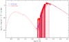 |
Fig. 1 Spectral energy distribution for a model without X-rays (blue curve) overplotted with those of a model including X-rays using the moderate illumination parameters (red dashed curve). |
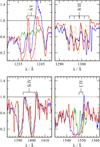 |
Fig. 2 Effect of including X-rays in the atmosphere calculations: The averaged observed normalized spectrum for selected UV lines (blue thin solid line) is compared to HD-PoWR models without (green solid line) as well as with moderate (red solid line) and strong X-ray illumination (brown dashed curve). |
3 Results
To a obtain starting model, we a calculated a non-HD model with the extended atomic data, but without any X-rays. Adopting the same notation as in Sander et al. (2017), where P(r) is the sum of the gas and turbulence pressure, ρ(r) is the density, and v(r) the wind velocity, we obtained a work ratio
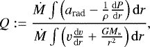 (5)
(5)
which is a measure for the integrated HD balance, of Q ≈ 1.05. As described in the previous section, the clumping stratification was also changed compared to Giménez-García et al. (2016), so that our model slightly differs from the empirical study in some parameters. The full list of input parameters we used in all HD models is given in Table 3. The models also differ in various parameters from those used in the study by Krtička et al. (2012), who derived a mass-loss rate using a comparable approach, but accounted in their METUJE code only for the pure CMF line force (see Krtička & Kubát 2010). Since they did not provide any emerging spectrum, we preferred the stellar parameters from the empirical results by Giménez-García et al. (2016).
Starting from the previously described non-HD model, the first hydrodynamically consistent model was calculated (first HD model). For this first model, no X-rays were included, so that we simulated the situation for an unperturbed B-star wind with stellar parameters similar to the donor of Vela X-1. This model is not only helpful for comparisons, it is also essential for establishing the (electron) temperature stratification Te (r) for our follow-up models, since we left Te(r) unchanged when we included X-rays. Fixing Te(r) is of course a simplification since the influence of the X-rays, on the ionization structure, for example, might change the temperature stratification. Nonetheless, this also avoids overestimating the changes in Te (r) since our X-ray inclusion is already rather approximate and not limited to a tiny NS source that would have a much smaller effect than our 1D treatment. Even the first non-X-ray model yields a relatively low terminal wind velocity of v∞ = 532 km s−1, thereby theoretically backing the empirically derived value of v∞ ≈ 700 km s−1 determined by Giménez-García et al. (2016). This is also in line with the results from Krtička et al. (2012), who obtained v∞ = 750 km s−1 in their model without X-rays. These values are notably lower than what was inferred from IUE observations by Dupree et al. (1980, ~ 1700 km s−1) and Prinja et al. (1990, ~ 1100 km s−1), but as demonstrated in Giménez-García et al. (2016), models with high velocities would significantly overestimate the observed UV line profiles. Furthermore, especially the population of C IV is significantly larger than for an unperturbed B star, resulting in a much stronger UV profile, as we discuss in Sect. 3.1.
Based on the first HD model, two more HD models were calculated, adopting the previously discussed X-ray parameters corresponding to LX ≈ 2.2 × 1033 erg s−1 and LX ≈ 6.7 × 1036 erg s−1, respectively.We refer to the two cases as “moderate” and “strong” illumination test cases in the following. For the moderate case, we used the same X-ray onset radius as Giménez-García et al. (2016), namely R0,1 ≡ d0 = 1.2 R*, while in the strong case, we used the X-rays from the moderate case plus an additional second component with an onset radius R0,2 = dNS = 1.8 R*. To avoid multiple indices, we use the terms d0 and dNS in all figures where these onset radii are outlined.
Since Giménez-García et al. (2016) used X-ray parameters that correspond to neither of these two cases, we also calculated a model with their X-ray parameters. However, these results were almost identical to our results when we used the LX that is motivated by eclipse measurements. Therefore, we refrain from discussing this additional X-ray HD model here more explicitly. Nevertheless, it is worth mentioning that the X-ray implementation in PoWR (see Sect. 2.3) does not necessarily lead to the same value of LX when the underlying atomic data and the clumping stratification are changed. While Giménez-García et al. (2016) have LX ≈ 5 × 1033 erg s−1, the HD model with the same R0, TX, and Xfill has LX ≈ 8 × 1034 erg s−1, meaning that the resulting X-ray luminosity is more than an order of magnitude higher. This is mainly an indirect effect of the slight change in the clumping stratification, which leads to a different onset. In our models, clumping starts earlier, in particular at a mean density that is about two orders of magnitude higher than the density in Giménez-García et al. (2016). Since a significant part of the emerging X-ray flux in our model stems from a wavelength regime where the wind is optically thin for X-rays, the higher clumping factor in the deeper layers becomes important and would have to be compensated for by a smaller X-ray filling factor if the same LX were to be kept. We instead decided to keep the Xfill from Giménez-García et al. (2016) for the moderate case and assumed Xfill = 2 for the additional component in the strong case, while adjusting the X-ray temperatures TX to obtain the required values of LX.
Input parameters for the Vela X-1 donor models.
3.1 X-ray sensitive UV features
Our first HD model without any X-rays yields v∞ ≈ 532 km s−1 together with logṀ = −6.19. As we show below, our two X-ray test cases affect the obtained terminal velocity, but leave the mass-loss rate almost unaffected. However, in all cases, the X-rays do significantly affect the ionization stratification in the wind and thus can have an imprint on the spectral lines that originate in the wind, most notably in the UV.
This is demonstrated in Fig. 2 for a selection of UV lines for four different ions, where we compare the averaged observed IUE spectrum with our different HD consistent models. The observational data we used are identical to those used by Giménez-García et al. (2016), where a more detailed description of the considered observations can be found. While Si III and Si IV are essentially unaffected in the case of moderate X-ray illumination, the absorption trough of the C IV doublet is significantly widened by an enhanced population of C IV in the wind. For N V, the effect is even more spectacular: Without X-rays, this ion is essentially absent in the outer wind, but the inclusion of X-rays offers an ionization source that then substantially populates N V, even when using just the LX from the moderate illumination model. The idea that X-rays are responsible for this effect goes back to Cassinelli & Olson (1979) after the discovery of C IV and N V in the Copernicus and Skylab spectra of stars (Snow & Morton 1976; Parsons et al. 1979), whose winds were too cool for these ionization stages in radiative equilibrium. Since Cassinelli & Olson (1979) assumed a coronal X-ray origin, the proper accounting for X-rays that affect the ionization balance in the stellar wind was only performed in later studies (e.g., Macfarlane et al. 1993, Macfarlane et al. 1994) despite the early discussions of donor wind changes caused by X-rays in the context of X-ray binaries (e.g., Basko & Sunyaev 1973; McCray & Hatchett 1975).
The changes in the ionization stages for our Vela X-1 donor wind model are visualized in Fig. 3, where we compare the relative ground-state populations for carbon and nitrogen. The leading ionization stage, that is the stage that most of the ions of an element populate, is also more or less unaffected when considering only the LX from the moderate illumination model. The reason is that the population numbers in the leading stage, that is, C III and N III here, were several orders of magnitude larger than the those of C IV or N V in the model without X-rays, and the amount of X-rays in the moderate illumination case is just not high enough to significantly deplete the lower stages. The change in the ionization balance sets in immediately where the X-rays are inserted in the moderate illumination case, namely at d0.
The whole ionization balance changes significantly for the model in which the strong LX is applied. Now the lower ionization stages become depleted outward of dNS, where the additional X-ray component is taken into account. The depletion even increases farther out at about r≳2dNS, where C V and N VI become the dominant ionization stage. However, the X-ray flux is still not high enough to populate even higher stages, such as C VI or N VII. We account for these high ionization stages in our calculations (cf. Table A.1), but their population is so small that they are far below the scale in Fig. 3.
Since the strong illumination case consists of two X-ray components, setting in at d0 and dNS, we see corresponding changes in the ionization trend at these radii. The third change in the trend at r≳2dNS does not reflect a change in the X-ray treatment, but instead indicates the region where the wind becomes transparent to X-rays. As the X-rays increasingly deplete the leading opacity sources such as He II or O III in outward direction, they essentially remove the material that would be able to absorb X-rays. When these lower stages are fully depleted, the wind becomes transparent at X-ray wavelengths and the leading ionization stages change significantly, for example, to He III or O VII.
The strong X-ray illumination also leaves quite a notable imprint on the UV lines in Fig. 2. The emission parts of C IV and N V lines become stronger and the blue edges of all P Cygni lines shrink, hinting at a lower wind velocity, which is indeed the case, as we show below when we discuss the stratification. Since the different amounts of X-ray illumination are a rough approximation of what we see from a system like Vela X-1 in different orbital phases, our resulting UV line profiles essentially mimic the so-called “Hatchett–McCray effect”, that is, an orbital modulation of the UV lines that is due to the change in position of the NS and its zone with higher ionization that is due to the X-rays. This was first discussed by Hatchett & McCray (1977) and has later indeed been confirmed for Vela X-1 by comparing UV spectra from different orbital phases (e.g., Kaper et al. 1993; van Loon et al. 2001). The change in the UV lines of our models also agrees qualitatively with the modeling results from van Loon et al. (2001), who used a radiative transfer code based on the so-called “Sobolev with exact integration” (SEI) method (Lamers et al. 1987). In this work we do not aim to reproduce the precise shapes of the UV line profiles. For this task, optically thick wind clumping in the radiative transfer calculations would also need to be considered, which is often discussed under the keywords “macroclumping” (e.g., Oskinova et al. 2007; Šurlan et al. 2013) or “porosity” (e.g., Owocki 2008; Sundqvist et al. 2014) in physical and velocity space, from which we refrain here as it is beyond the scope of the present work.
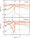 |
Fig. 3 Relative population numbers for the ground-state ion levels of carbon (upper panel) and nitrogen (lower panel) in the HD models with moderate LX (red curve), strong LX (brown dashed curve), and without X-rays (green curve). |
3.2 Mass-loss rates
A compilation of the results from the hydrodynamically-consistent wind models for the donor star of Vela X-1 is presented in Table 2, where we list all three models and compare them to the empirical model with prescribed v(r) by Giménez-García et al. (2016). The mass-loss rates of all three HD models differ by less than 0.1 dex, while the terminalwind velocities vary as a result of the different X-ray illumination. While we discuss the stratification details in the following section, we can conclude at this point that the X-rays do not strongly affect the layers of the critical point and below. The radius of the critical point rc remains about the same for the moderate X-ray illumination case and moves only slightly inward for the strong illumination case, resulting in a tiny increase in the mass-loss rate. The latter is exactly in line with the findings of MacGregor & Vitello (1982) for HMXBs where the authors used a simpler Sobolev-based model. It also agrees with studies that have been performed for intrinsic X-rays in single-star winds (e.g., Krtička & Kubát 2009).
Our value of the mass-loss rate in the non-X-ray model is 6.5 × 10⁻⁷ M⊙ yr−1. This is slightly more than a factor of two lower than found by Krtička et al. (2012), namely 1.5 × 10⁻⁶ M⊙ yr−1. However, their modeling assumed a smooth wind, while we used a depth-dependent microclumping approach with D∞= 11. While a simple comparison by multiplying our Ṁ with  yields 2.1 × 10⁻⁶ M⊙ yr−1 would provide a good agreement, this diagnostic is only valid for wind lines that scale with ρ2. Moreover, Muijres et al. (2011) discovered that for a microclumping approach, the mass-loss rate should even increase compared to the unclumped situation, although the recent CMF-based calculations by Petrov et al. (2016) might question this. The reasons that our mass-loss rate is lower than that of Krtička et al. (2012) likely lies in the different stellar parameters considered in the calculation. Even though both models use more or less the same log g, the luminosity resulting from the parameters in Krtička et al. (2012) is about 40% higher, which likely propagates into the higher mass-loss rate.
When we compare our result of logṀ = −6.19 to the predictions from Vink et al. (2000, Vink et al. 2001) assuming solar metallicity, their prediction of − 5.06 is more than an order of magnitude higher. For the stellar parameters from Krtička et al. (2012), the prediction would be − 5.61, which is also higher than obtained by Krtička et al. (2012), but only by about 0.2 dex. The main reason for the larger discrepancy with the predictions from Vink et al. (2000, Vink et al. 2001) is our lower temperature of T2∕3 = 23.5 kK. This is located between the two bistability jumps identified in Vink et al. (1999), while the 27 kK assumed by Krtička et al. (2012) is already above the higher bistability jump implemented in their formula. The steep increase in mass-loss rates when transitioning to cooler temperatures in the calculations from Vink et al. (1999) is not seen in our model. However, the observed bistability according to Lamers et al. (1995) should occur around 21 kK, and the recent calculations from Petrov et al. (2016) also found it in a similar range, which would place even our value of T2∕3 still on the hotter side. Unfortunately, Petrov et al. (2016) does not offer models with 20 M⊙ around our T2∕3, which would have allowed for a direct comparison of Ṁ. In any case, the donor star of an HMXB is a particular situation and although most abundances in our model are assumed to be solar, there is a significant nitrogen enrichment and carbon depletion as derived by Giménez-García et al. (2016), which we take into account, so the comparison with models based on scaled main-sequence compositions is certainly limited. Nevertheless, our models provides a first interesting test case for the bistability jump regime, which we discuss in the context of the driving ions in Sect. 3.5 in more detail.
3.3 Stratification
In an HD PoWR model, the outward and inward forces balance each other throughout the whole atmosphere, thus providing a self-consistent stratification. A visual check for the success of the solution method can be made by plotting the different accelerations, namely the total radiative acceleration arad(r), the acceleration from gas pressure as a result of temperature and turbulence apress(r), the gravitational acceleration g(r), and the inertia 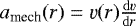 . This is shown in Fig. 4 for the model accounting for moderate X-ray illumination. The sum of arad and apress matches the sum of g and amech throughout the atmosphere, and thus our model is indeed hydrodynamically consistent.
Inspection of the contributions from the different accelerations in Fig. 4 reveals that the general picture is very similar to what we obtained for the significantly hotter O supergiant in Sander et al. (2017). In the wind, only the line acceleration and Thomson scattering are important, while in the inner subsonic regime, the gas pressure and the contributions from the continuum opacities from bound-free transitions have also to be considered. However, the curve shapes differ in detail, and the increase of arad beyond the critical point is significantly shallower than in the case of the O supergiant (cf. Fig. 6 in Sander et al. 2017). This is due to the different ions that contribute in the temperature regime of an early-B supergiant with T* = 25.5 kK compared to the 42 kK of the O star discussed in Sander et al. (2017). The detailed elemental contributions to the driving are discussed in Sect. 3.5.
A comparison of the velocity field v(r) from Giménez-García et al. (2016) using a prescribed β-law connected to a consistent hydrostatic solution (see Sander et al. 2015, for technical details) and from our HD consistent model is shown in Fig. 5. While we see a sharp increase for v(r) in the model from Giménez-García et al. (2016) around and outward of the sonic point, which marks our critical point in the HD case, the increase is more moderate for the self-consistent HD models. A similar situation occurred forthe O supergiant model in Sander et al. (2017) and is likely related to two things: first, the β-value used for theprescribed law is – if not simply adopted but motivated by observations – typically inferred from Hα. Second, v(r) in the region around the connection point between the quasi-hydrostatic layers and the β-law regime can significantly violate the acceleration balance we aim at with our HD models. When these models are used to obtain empirical stellar and wind parameters, this is usually not a problem, but as soon as conclusions are to be drawn from the detailed stratification, this can lead to errors, most notably in this transition regime.
A closer look reveals that all HD solutions behave rather similar in the inner wind near the critical point, but in the outer layers, the effects of the different amount of X-rays become clearly noticeable. In the model with moderate X-ray illumination, the amount of X-rays is just enough to ionize the wind such that the population of some of the driving ions such as N V increases and additional driving is provided. However, when the amount of X-rays becomes too high, as we see in the strongly X-ray illuminated model, there is so much ionization that important driving ions are depopulated, causing a sharp decrease in the line acceleration in the outer wind. This effect is also illustrated in Fig. 6, where we compare the wind accelerations for all three HD solutions. Here, we further note that the flattening of the velocity field for the strong illuminationcase seen in Fig. 5 is an artifact that is due to our technical limitations to monotonic velocity fields in the CMF radiative transfer rooted in the structure of the frequency boundary together with the applied elimination scheme (for more details, see Mihalas et al. 1975, especially their Appendix A). Since the normalized wind acceleration drops below unity here, we would have a deceleration in reality and thus an even lower terminal velocity than obtained in this work, which we cannot model because of the limitation to monotonic velocity fields. Interestingly, Kaper et al. (1993) suggested a have-monotonic velocity field for the donor wind of Vela X-1 because they had difficulties to model the changes of the UV lines when assuming a monotonic v(r), but they discussed this with regard to wind-intrinsic instabilities and not wind deceleration that is due to X-ray ionization. In the work of Krtička et al. (2012), the velocity in the direction toward the NS stops to increase much farther inward than in our model. The reasons are hard to determine, since not only their X-ray treatment, but also their radiative transfer treatment are entirely different. In their X-ray models, they use the Sobolev line acceleration corrected with factors obtained from their CMF-based calculation in the non-X-ray case. They furthermore do not seem to consider the acceleration due to Thomson scattering, which – unlike the line acceleration – does not break down in our models. In any case, Fig. 5 demonstrates that in all models the wind is accelerated to velocities higher than the local escape speed, allowing the material to leave the star even if no further acceleration were to occur. Interestingly, for Vela X-1, this is coincidentally just around or slightly beyond the radius where the NS is located. A rather slow wind at this distance fosters the accretion of wind material by the compact object, as we discuss in more detail in Sect. 3.4. Furthermore, in the strong X-ray illumination model, the wind speed does not surpass the escape speed at R* of vesc = 521 km s−1, even when we consider the reduction due to Γe, which would decrease the escape speed to 420 km s−1. In the other two cases, we obtain a ratio v∞∕vesc ≈ 1.3 when we account for Γe in vesc. This ratio is typical for the regime between the two bistability jumps (e.g., Lamers et al. 1995; Vink et al. 1999), which is especially interesting as our mass-loss rate would be associated with the regime above the jumps.
Although the radiative acceleration drops for r≳2dNS, Fig. 6 also illustrates that it does not vanish completely, and the wind might therefore not be shut off completely, even in the strongly ionized region. Our quite approximate X-ray treatment and the fixed temperature structure might be a caveat here, but it is noteworthy that the large breakdown of the acceleration and thus the strongest effect of the X-rays does not occur at the distance of the NS, but instead much farther outside for r ≳ 3 R*≈ 2dNS, where the stratification also becomes optically thin for X-ray wavelengths and the ionization balance changes, as discussed in Sect. 3.1. A more sophisticated treatment of the situation is needed to verify these results, but this might have interesting consequences for the proper wind treatment in multidimensional time-dependent HD simulations of HMXBs.
The (electron) temperature stratification Te(r) for all HD models is displayed in Fig. 7, where we also show the stratification from Giménez-García et al. (2016) for comparison. The results do not differ much, but the HD model is slightly hotter in the inner part and has minor non-monotonic parts in the outer wind. The shift in the optically thick part likely arises from the lower microturbulent velocity assumed in the HD calculations, which we fixed in the main iteration at the more “canonical” 10 km s−1 for B-supergiants (e.g., Lanz & Hubeny 2007) compared to 30 km s−1 in Giménez-García et al. (2016). Furthermore, the region between Rcrit and R2∕3 is smoother, which likely results from the fact that the HD-stratification avoids artifacts that can arise when the velocity fields of the subsonicand the wind regime are connected. We note that both studies neglected the changes in the electron temperature structure that are due to X-rays.
The stratifications from all three HD consistent wind models are provided as tables in Appendix B.
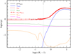 |
Fig. 4 Detailed acceleration stratification for the HD consistent model using the moderate X-ray flux. The wind acceleration (thick red diamond line) is compared to the repulsive sum of inertia and gravitational acceleration g(r) (black line). The input parameters of the model are given in Table 3, while the resulting quantities are listed in Table 2. In order to properly handle the various scales, this is a double-logarithmic plot with all acceleration terms normalized to g(r). |
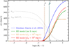 |
Fig. 5 Velocity field for Vela X-1 from Giménez-García et al. (2016) compared to the fields from the HD consistent models presented in this work using different X-ray fields. The orange line marks the location of the NS at a radius of dNS = 1.8 R* from the center of the donor, while the colored dashed lines denote the location of the critical point in the corresponding HD models. The grey dashed lines denote the escape speed vesc (r) without (large dashes) and with (small dashes) accounting for the reduction due to Γe. |
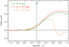 |
Fig. 6 Comparison of the total wind acceleration – normalized to g(r) – for the three HD consistent models using different amounts of X-ray illumination. |
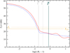 |
Fig. 7 Electron temperature stratification for the HD consistent models (red solid curve) compared to those of a model with a prescribed wind stratification (blue dashed curve) based on Giménez-García et al. (2016). Horizontal lines mark T* and T2∕3 for the HD-models. Vertical lines denote R2∕3 as well as the critical radius for the HD-model without X-rays and the distance of the NS. |
3.4 Accretion estimation
In the so-called “wind-fed HMXBs”, the wind of the donor star is accreted by the compact object, in our case, an NS star. The empirical results from Giménez-García et al. (2016) place Vela X-1 in the so-called “direct accretion regime”, using both the vwind-Pspin and the vwind-Ṁ planes to visualize the scheme from Bozzo et al. (2008). This scheme compares the relative positions of the NS magnetospheric radius with its accretion and corotation radii. The equations for transitions between different accretion regimes can be expressed with the help of the donor’s wind parameters. Since our results for the mass-loss rate in general confirm the findings of Giménez-García et al. (2016) and the wind velocity at the distance of the NS is even slightly lower than the one inferred from their prescribed law, the assumption that Vela X-1 is set in the direct accretion regime is corroborated by our results. For this case, we can expect the X-ray luminosity LX to be roughly on the order of the accretion luminosity Lacc, which we estimate through Bondi–Hoyle–Lyttleton (BHL) accretion (Hoyle & Lyttleton 1939; Bondi & Hoyle 1944; Davidson & Ostriker 1973). A more detailed discussion of BHL accretion and the different accretion regimes can be found in the recent review by Martínez-Núñez et al. (2017).
The Bondi–Hoyle radius or “accretion radius”
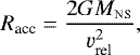 (6)
(6)
describes the radius around the NS within which wind material can be captured and accreted. MNS denotes the mass of the NS, and G is the gravitational constant. The relevant velocity for Racc is the relative velocity vrel between the NS and the donor wind, resulting from the radial wind velocity v(r = dNS) and the orbital velocity of the NS, vorb. For a circular orbit, which is quite a good approximation for the case of Vela X-1 (e≲0.1, see Table 1), the vector calculation simplifies to
 (7)
(7)
When estimating the relative velocity, a common assumption is to use vrel≈ v(dNS) assuming that the orbital velocity is much lower than the wind velocity ( ). Since the shape of the velocity field is usually unknown, assuming v(dNS) ≈ v∞ is sometimes used as well, which wouldallow us to replace vrel with v∞ in Eq. (6). However, both assumptions cannot be taken for granted for a particular system and thus can lead to significant errors in the accretion estimation if used inadvertently. Typical orbital separations are dNS ≈ 2 R*, at which it is by no means guaranteed that the wind has already reached its terminal velocity.
In the case of Vela X-1, the NS seems to be located even slightly closer. Using the velocity field from our model with moderate X-ray illumination, we predict a value of v(dNS) that is almost an order of magnitude lower than v∞, meaning that this would be causing a huge error due the steep velocity dependence, as we show in the further calculation. For other systems, this error might be smaller, but overestimating vrel by a factor of 2 would be rather typical when assuming v(dNS) ≈ v∞. Second, the low wind velocity at the distance of the NS also means that the assumption  is not true. With the prescribed velocity field, Giménez-García et al. (2016) have reported vorb ≈ v(dNS). The HD consistent solution now predicts that the wind velocity at the location of the NS is even lower than the orbital speed of the compact object. Thus Eq. (7) yields in our case vrel ≈ 300 km s−1.
Assuming that the potential energy from the accreted matter is completely converted into X-rays, we obtain the accretion luminosity,
 (8)
(8)
with RNS denoting the radius of the NS and Ṁacc the mass accretion rate. Assuming direct wind accretion, the latter can be expressed as
 (9)
(9)
where ζ is a numerical factor introduced to correct for radiation pressure and finite gas cooling. For moderately luminous X-ray sources, this is commonly taken as ζ ≡ 1. Approximating the density ρ(dNS) with the density from a stationary spherically symmetric wind, we can write
 (10)
(10)
This allows us to rewrite Eq. (9) such that we can express the accretion rate with the wind mass-loss rate of the donor star,
 (11)
(11)
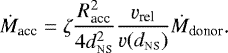
Now plugging Eq. (11) into Eq. (8) and replacing Racc with the help of Eq. (6), we obtain

which eventually allows us to estimate Lacc using our results. Applying typical values for the NS (MNS = 1.4 M⊙, RNS = 12 km, dNS = 1.8 R*, vNS = 281 km s−1) and inferring a value of v(dNS) ≈ 100 km s−1 from our HD model, which we essentially find regardless of the particular X-ray illumination, we find
 (15)
(15)
with the small range spanned by the mass-loss rates derived from no (lower value) and strong (higher value) X-ray illumination. This is on the order of what we used as LX in our strong illumination test case. Owing to the lower value of v(dNS) compared to Giménez-García et al. (2016), our value of Lacc is almost an order of magnitude higher, resulting from the fact that Lacc roughly scales with the inverse of this quantity to the fourth power. Although the average X-ray luminosity ⟨LX ⟩≃ 4.5 × 1036 erg s−1 (Sako et al. 1999; Fürst et al. 2010) is also an order of magnitude lower, our estimate is still remarkably consistent given that we assumed accretion to be so efficient that all energy is converted into X-ray luminosity. Since the BHL estimate is likely an upper limit, as indicated by simulations performed for accretion in binaries (e.g., Theuns et al. 1996), it is common to introduce an accretion efficiency parameter  – sometimes also termed transformation factor – which is typically assumed to be around
  (e.g., Negueruela 2010; Oskinova et al. 2012). In our case, a value of 0.1 would lead to an excellent agreement between our estimate and the observed ⟨LX ⟩.
3.5 Wind driving and the bistability jump
A more detailed look into the wind driving is possible through studying the contributions of the various elements to the radiative acceleration, as illustrated in Fig. 8 for the model using the moderate X-ray flux. At solar metallicity, the iron opacities are the main line contributions to the driving until the sonic point and farther outward up to about 2 R*. While this appears to be rather similar to the much hotter O-supergiant (ζ Pup) model from Sander et al. (2017), it is noteworthy that the iron contribution already outweighs the free electron (Thomson) scattering contribution at the sonic point in the case of Vela X-1. This is not the case for ζ Pup, where the main ion contributing to the iron acceleration fraction is Fe V instead of Fe III here, which is shown in Fig. 9, where the relative contributions of the various ions in the wind are plotted. The different temperature and thus ionization regime also leads to the differences in the list of elements that provide major contributions in the outer wind: After a few R*, sulfur, nitrogen, and the iron group (in descending order) all provide between 15% and 20% of the radiative force. Slightly smaller contributions stem from Si and C. Oxygen provides about 5%, which is already below the Thomson contribution. Interestingly, it is followed by hydrogen – because of its significant continuum contribution – and then several elements (Al, Cl, P, and Ar) that contribute on a percentage level. The driving influence of K is already two orders of magnitude lower than that of the leading elements and below the basically negligible gas pressure. The remaining elements (He, Ne, Mg, andCa) contribute even less and thus can be neglected with regard to driving. However, as the comparison with the ζ Pup model from Sander et al. (2017) illustrates, we have to be cautious about generalizing these results. The influence of the various elements strongly depends on the abundances and the ionization stages, and thus the picture can change drastically when transitioning to other temperature and/or abundance regimes.
As previously mentioned in Sect. 3.2, our self-consistent model provides an interesting test-case for the discussion of the (hot) bistability jump, which was originally discovered in wind models for P Cyg by Pauldrach & Puls (1990) and was later observationally corroborated by Lamers et al. (1995), who found a discontinuity in the v∞ ∕vesc ratio around an effective temperatureof 21 kK. Pauldrach & Puls (1990) have attributed the nature of the jump to a change in the leading ionization, which can have a significant effect on the driving. Vink et al. (1999) were able to find the bistability jump in their theoretical models by obtaining the radiative acceleration through Monte Carlo calculations, but at the slightly higher temperature of 25 kK. Using grids of CMFGEN models and interpolating at Q = 1, Petrov et al. (2016) predicted the region of the jump to be located between 22.5 kK and 20 kK. In both approaches, the change in the ionization structure is identified as the origin of the jump. Detailed knowledge about the exact locations and the intensity of the bistability jumps is very important, not only for our understanding of key objects like B-hypergiants (e.g., Clark et al. 2012; Oskinova et al. 2017) but also for correctly modeling the evolution of massive OB stars in general, for example, as recently demonstrated by Keszthelyi et al. (2017).
With our result of T2∕3 = 23.5 kK, we are still very close to the bistability jump, which is also indicated by the unusual combination of a low Ṁ combined with v∞∕vesc ≈ 1.3 (see Sect. 3.3). In the model without X-rays, Fe IV is the leading Fe ion with regard to the population numbers, while Fig. 10 clearly shows that its contribution to the driving in the wind is clearly minor compared to Fe III, which was also found in calculations from both Vink et al. (1999) and Petrov et al. (2016). While the results visualized in Figs. 8 and 9 are for a moderate X-ray illumination, the results for the non-X-ray model differ only in the details, as can be seen when comparing Fig. 9 with Fig. 10. The absence of all the higher ions (C IV, N IV, N V, also O IV and Cl IV at greater distance) in the wind part is conspicuous, since these ions are not significantly populated without the X-ray channel. In absolute numbers, the picture is very similar to Fig. 8, but without X-rays, the contributions of C, N, O, Si, and S are smaller, and Si and S are only mildly affected. Nevertheless, this change is enough to barely make iron – or the iron group elements, to be more exact – the leading element now.
From the calculations of Petrov et al. (2016), the contribution of CNO elements to the total work ratio was also derived. With our detailed calculations and their visualized results in Figs. 8 and 10, we can now not only verify their finding that the combined CNO contribution outweighs the iron-driving contribution in our temperature regime, but investigate this also in a depth-dependent manner, revealing that this is only true for the outer wind regime at r ≳ 3 R*, while Fe III and electron scattering are the dominant drivers below, down to the regime around the sonic point. We also discovered the important influence of Si and S in accelerating the wind, in particular S III and Si III, but also S IV and Si IV to a lesser degree, which was not noted by Petrov et al. (2016) although they included these elements in their calculations.Given these results and the significant differences between the contributions of C, N, and O, we therefore conclude that it is dangerous to consider the CNO elements alone as important drivers and disregard the importance of other elements such as S and Si. While S and N have comparable influences, the influence of O is about a factor of three lower. Of course we have to keep in mind that nitrogen is enriched while oxygen is slightly depleted, which is likely a result of the CNO cycle, but carbon is depleted as well, even much more strongly than oxygen, and still it has about twice the driving influence of oxygen in the wind. These deviations from the solar composition might be another reason why our results differ from predictions such as those in Vink et al. (2000). We plan to investigate the whole topic of detailed driving contributions in more detail in future studies.
We finally consider the origin of the “bump” structure that occurs in the radiative acceleration regardless of X-ray illuminationshortly below the sonic point. This structure, which is most notably seen in the contributions from iron, hydrogen, and electronscattering, does not originate from any major ionization change or non-monotonic feature in the temperature structure, but instead stems from the increase in the clumping factor in this region. Below the bump, we have D ≈ 1, while we have D ≈ 7 at the critical point. While the further increase outward does not leave a notable substructure on the radiative acceleration, the onset of the clumping does, in contrast to our O supergiant model in Sander et al. (2017), even though the clumping increase there started below the critical point as well. The influence of the clumping stratification on the radiative acceleration is another topic that has to be studied in more detail in the future.
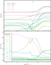 |
Fig. 8 Absolute (upper panel) and relative (lower panel) contributions to the radiative acceleration from the different elements considered in the HD consistent atmosphere model incorporating the moderate X-ray flux. The total radiative acceleration and the acceleration due to gas pressure are also shown in the upper panel for comparison. The lower panel shows the fraction that electron scattering (pink solid curve), and the various elements contribute to the total radiative acceleration. |
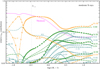 |
Fig. 9 Relative contributions to the radiative acceleration from the different ions (colored curves with various symbols) and due to scattering by free electrons (pink solid curve) for the HD consistent model with moderate X-ray illumination (cf. Table 2). Only ions that contribute at least 1% to the radiative acceleration are shown. For better visibility of the various contributions on a percentage level, the y-axis is shown on a logarithmic scale. |
4 Conclusions
We constructed HD consistent PoWR models for the donor star of Vela X-1, HD 77581, thereby for the first time applying our recently introduced next-generation PoWR models (Sander et al. 2017) to the regime of early-B supergiants. The values of the stellar parameters were motivated by the previous empirical study from Giménez-García et al. (2016), and the resulting models reproduce the overall spectral appearance of the donor star. Three HD consistent models using different levels of X-ray illuminations demonstrate the effects of the X-rays that arise from accretion onto the NS in the Vela X-1 system on the donor star wind.
Our atmosphere models prove that the low terminal velocity derived by Giménez-García et al. (2016) is consistent with the radiative acceleration provided by the radiation of the donor star, in line with earlier predictions by Krtička et al. (2012). In the inner wind region, our hydrodynamical models yield a stratification that is notably different from what is obtained when a prescribed β-law is used. Our calculations furthermore reveal that a certain amount of X-rays influences the ionization balance such that additional driving is provided in the outer wind, and the terminal velocity is increased by about 10% compared to a similar donor star without X-rays. However, when the X-ray illumination is too high, a breakdown of the acceleration occurs in the outer wind. It is noteworthy that this breakdown does not occur already at the distance of the NS dNS, but instead much farther out after r ≳ 3 R*≈ 2dNS. Nevertheless, owing to the restriction to a stationary 1D description of the wind and a rather approximate X-ray treatment, this result should be taken with care.
Our calculations confirm the empirically derived mass-loss rate of the donor star of Vela X-1 of log Ṁ ≈−6.2 assuming a depth-dependent microclumping with D∞ = 11. The X-ray illumination has only very little influence on the wind mass loss, potentially increasing the rate by up to 0.1 dex in the direction toward the NS. The wind velocity in the inner wind and especially at the distance of the NS v(dNS) ≈ 100 km s−1 is lower than typically estimated from prescribed β-laws. Our obtained v(dNS) is lower than the orbital speed of the NS, but an estimate assuming direct BHL accretion yields excellent agreement between the mean observed X-ray luminosity of Vela X-1 and our prediction. Tables with the stratifications from all the HD consistent models are provided in Appendix B.
A detailed inspection of the driving contributions reveals that a plethora of ions from more than ten different elements need to be considered to properly reconstruct the full radiative wind acceleration. The leading ion in our early B-type supergiant wind is Fe III, which contributes about 15% in the case of a moderate X-ray illumination. In the outer wind, S III reaches an almost comparable fraction, followed by Si III and C III which contribute about 10% in the wind. Although the general picture of the B-supergiant wind shows similarities to our previous O-supergiant results (Sander et al. 2017), the detailed contributions are significantly different because of the different stellar parameters. Further studies are required before more general conclusions should be drawn.
Acknowledgements
We would like to thank the anonymous referee for the insightful questions and suggestions that helped to strengthen this paper. A.A.C.S. is supported by the Deutsche Forschungsgemeinschaft (DFG) under grant HA 1455/26. T.S. acknowledges support from the German “Verbundforschung” (DLR) grant 50 OR 1612. This research made use of the SIMBAD and VizieR databases, operated at CDS, Strasbourg, France. This publication was motivated by a team meeting sponsored by the International Space Science Institute at Bern, Switzerland. We acknowledge support from the Faculty of the European Space Astronomy Centre (ESAC).
Appendix A: List of atomic data used in the stellar atmosphere models
Atomic data used in the HD models.
Appendix B: Stratifications of our hydrodynamcially consistent wind models for the donor star of Vela X-1
Stratification for the atmosphere model without any X-ray illumination.
Stratification for the atmosphere model with moderate X-ray illumination (LX ≈ 1033 erg s−1 ).
Stratification for the atmosphere model with strong X-ray illumination (LX ≈ 1037 erg s−1).
References
- Allen, C. W. 1973, Astrophysical Quantities, 3rd ed. (London: University of London, Athlone Press) [Google Scholar]
- Asplund, M., Grevesse, N., Sauval, A. J., & Scott, P. 2009, ARA&A, 47, 481 [NASA ADS] [CrossRef] [Google Scholar]
- Basko, M. M., & Sunyaev, R. A. 1973, Ap&SS, 23, 117 [NASA ADS] [CrossRef] [Google Scholar]
- Baum, E., Hamann, W.-R., Koesterke, L., & Wessolowski, U. 1992, A&A, 266, 402 [NASA ADS] [Google Scholar]
- Bildsten, L., Chakrabarty, D., Chiu, J., et al. 1997, ApJS, 113, 367 [NASA ADS] [CrossRef] [Google Scholar]
- Blondin, J. M., & Pope, T. C. 2009, ApJ, 700, 95 [NASA ADS] [CrossRef] [Google Scholar]
- Blondin, J. M., Kallman, T. R., Fryxell, B. A., & Taam, R. E. 1990, ApJ, 356, 591 [NASA ADS] [CrossRef] [Google Scholar]
- Blondin, J. M., Stevens, I. R., & Kallman, T. R. 1991, ApJ, 371, 684 [NASA ADS] [CrossRef] [Google Scholar]
- Bondi, H., & Hoyle, F. 1944, MNRAS, 104, 273 [NASA ADS] [CrossRef] [Google Scholar]
- Bozzo, E., Falanga, M., & Stella, L. 2008, ApJ, 683, 1031 [NASA ADS] [CrossRef] [Google Scholar]
- Cassinelli, J. P., & Olson, G. L. 1979, ApJ, 229, 304 [NASA ADS] [CrossRef] [Google Scholar]
- Castor, J. I., Abbott, D. C., & Klein, R. I. 1975, ApJ, 195, 157 [NASA ADS] [CrossRef] [Google Scholar]
- Chodil, G., Mark, H., Rodrigues, R., Seward, F. D., & Swift, C. D. 1967, ApJ, 150, 57 [NASA ADS] [CrossRef] [Google Scholar]
- Clark, J. S., Najarro, F., Negueruela, I., et al. 2012, A&A, 541,A145 [NASA ADS] [CrossRef] [EDP Sciences] [Google Scholar]
- Davidson, K., & Ostriker, J. P. 1973, ApJ, 179, 585 [NASA ADS] [CrossRef] [Google Scholar]
- Dupree, A. K., Gursky, H., Black, J. H., et al. 1980, ApJ, 238, 969 [NASA ADS] [CrossRef] [Google Scholar]
- Falanga, M., Bozzo, E., Lutovinov, A., et al. 2015, A&A, 577, A130 [NASA ADS] [CrossRef] [EDP Sciences] [Google Scholar]
- Fraser, M., Dufton, P. L., Hunter, I., & Ryans, R. S. I. 2010, MNRAS, 404, 1306 [NASA ADS] [Google Scholar]
- Fürst, F., Kreykenbohm, I., Pottschmidt, K., et al. 2010, A&A, 519, A37 [NASA ADS] [CrossRef] [EDP Sciences] [Google Scholar]
- Giménez-García, A., Shenar, T., Torrejón, J. M., et al. 2016, A&A, 591, A26 [Google Scholar]
- Gräfener, G., Koesterke, L., & Hamann, W.-R. 2002, A&A, 387, 244 [NASA ADS] [CrossRef] [EDP Sciences] [Google Scholar]
- Hamann, W., & Koesterke, L. 1998, A&A, 335, 1003 [NASA ADS] [Google Scholar]
- Hamann, W.-R., & Gräfener, G. 2003, A&A, 410, 993 [NASA ADS] [CrossRef] [EDP Sciences] [Google Scholar]
- Hatchett, S., & McCray, R. 1977, ApJ, 211, 552 [NASA ADS] [CrossRef] [Google Scholar]
- Hauschildt, P. H., & Baron, E. 2006, A&A, 451, 273 [NASA ADS] [CrossRef] [EDP Sciences] [Google Scholar]
- Hauschildt, P. H., & Baron, E. 2014, A&A, 566, A89 [NASA ADS] [CrossRef] [EDP Sciences] [Google Scholar]
- Howarth, I. D., Siebert, K. W., Hussain, G. A. J., & Prinja, R. K. 1997, MNRAS, 284, 265 [NASA ADS] [CrossRef] [Google Scholar]
- Hoyle, F., & Lyttleton, R. A. 1939, Proc. Camb. Philos. Soc., 35, 405 [Google Scholar]
- Kaper, L., Hammerschlag-Hensberge, G., & van Loon J. T. 1993, A&A, 279, 485 [NASA ADS] [Google Scholar]
- Keszthelyi, Z., Puls, J., & Wade, G. A. 2017, A&A, 598, A4 [NASA ADS] [CrossRef] [EDP Sciences] [Google Scholar]
- Kreykenbohm, I., Wilms, J., Kretschmar, P., et al. 2008, A&A, 492, 511 [NASA ADS] [CrossRef] [EDP Sciences] [Google Scholar]
- Krtička, J., & Kubát, J. 2009, MNRAS, 394, 2065 [NASA ADS] [CrossRef] [Google Scholar]
- Krtička, J., & Kubát, J. 2010, A&A, 519, A50 [NASA ADS] [CrossRef] [EDP Sciences] [Google Scholar]
- Krtička, J., Kubát, J., & Skalický, J. 2012, ApJ, 757, 162 [NASA ADS] [CrossRef] [Google Scholar]
- Krtička, J., Kubát, J., & Krtičková I. 2015, A&A, 579, A111 [NASA ADS] [CrossRef] [EDP Sciences] [Google Scholar]
- Kubát, J. 2001, A&A, 366, 210 [NASA ADS] [CrossRef] [EDP Sciences] [Google Scholar]
- Kubát, J., Puls, J., & Pauldrach, A. W. A. 1999, A&A, 341, 587 [NASA ADS] [Google Scholar]
- Kudritzki, R.-P., & Puls, J. 2000, ARA& A, 38, 613 [Google Scholar]
- Lamers, H. J. G. L. M., Cerruti-Sola, M., & Perinotto, M. 1987, ApJ, 314, 726 [NASA ADS] [CrossRef] [Google Scholar]
- Lamers, H. J. G. L. M., Snow, T. P., & Lindholm, D. M. 1995, ApJ, 455, 269 [NASA ADS] [CrossRef] [Google Scholar]
- Lanz, T., & Hubeny, I. 2007, ApJS, 169, 83 [CrossRef] [Google Scholar]
- Lucy, L. B. 1964, SAO Special Report, 167, 93 [NASA ADS] [Google Scholar]
- Macfarlane, J. J., Waldron, W. L., Corcoran, M. F., et al. 1993, ApJ, 419, 813 [NASA ADS] [CrossRef] [Google Scholar]
- Macfarlane, J. J., Cohen, D. H., & Wang, P. 1994, ApJ, 437, 351 [NASA ADS] [CrossRef] [Google Scholar]
- MacGregor, K. B., & Vitello, P. A. J. 1982, ApJ, 259, 267 [NASA ADS] [CrossRef] [Google Scholar]
- Manousakis, A., & Walter, R. 2015, A&A, 584, A25 [NASA ADS] [CrossRef] [EDP Sciences] [Google Scholar]
- Martínez-Núñez, S., Torrejón, J. M., Kühnel, M., et al. 2014, A&A, 563, A70 [NASA ADS] [CrossRef] [EDP Sciences] [Google Scholar]
- Martínez-Núñez, S., Kretschmar, P., Bozzo, E., et al. 2017, Space Sci. Rev., 212, 59 [NASA ADS] [CrossRef] [Google Scholar]
- McCray, R., & Hatchett, S. 1975, ApJ, 199, 196 [NASA ADS] [CrossRef] [Google Scholar]
- Mihalas, D., Kunasz, P. B., & Hummer, D. G. 1975, ApJ, 202, 465 [NASA ADS] [CrossRef] [Google Scholar]
- Muijres, L. E., de Koter, A., Vink, J. S., et al. 2011, A&A, 526, A32 [Google Scholar]
- Nagase, F., Zylstra, G., Sonobe, T., et al. 1994, ApJ, 436, L1 [NASA ADS] [CrossRef] [Google Scholar]
- Negueruela, I. 2010, in ASP Conf. Ser., 422, 57 [NASA ADS] [Google Scholar]
- Oskinova, L. M., Hamann, W.-R., & Feldmeier, A. 2007, A&A, 476, 1331 [NASA ADS] [CrossRef] [EDP Sciences] [Google Scholar]
- Oskinova, L. M., Feldmeier, A., & Kretschmar, P. 2012, MNRAS, 421, 2820 [NASA ADS] [CrossRef] [Google Scholar]
- Oskinova, L. M., Huenemoerder, D. P., Hamann, W.-R., et al. 2017, ApJ, 845, 39 [NASA ADS] [CrossRef] [Google Scholar]
- Owocki, S. P. 2008, in Clumping in Hot-Star Winds, eds. W.-R. Hamann, A. Feldmeier, & L. M. Oskinova (Potsdam: Universitätsverlag Potsdam), 121 [Google Scholar]
- Parsons, S. B., Wray, J. D., Henize, K. G., & Benedict, G. F. 1979, in IAU Symp., 83, 95 [NASA ADS] [Google Scholar]
- Pauldrach, A. W. A., & Puls, J. 1990, A&A, 237, 409 [NASA ADS] [Google Scholar]
- Petrov, B., Vink, J. S., & Gräfener, G. 2016, MNRAS, 458, 1999 [NASA ADS] [CrossRef] [Google Scholar]
- Prinja, R. K., Barlow, M. J., & Howarth, I. D. 1990, ApJ, 361, 607 [NASA ADS] [CrossRef] [Google Scholar]
- Sako, M., Liedahl, D. A., Kahn, S. M., & Paerels, F. 1999, ApJ, 525, 921 [NASA ADS] [CrossRef] [Google Scholar]
- Sander, A., Shenar, T., Hainich, R., et al. 2015, A&A, 577, A13 [NASA ADS] [CrossRef] [EDP Sciences] [Google Scholar]
- Sander, A. A. C., Hamann, W.-R., Todt, H., Hainich, R., & Shenar, T. 2017, A&A, 603, A86 [NASA ADS] [CrossRef] [EDP Sciences] [Google Scholar]
- Sato, N., Hayakawa, S., Nagase, F., et al. 1986, PASJ, 38, 731 [NASA ADS] [Google Scholar]
- Schulz, N. S., Canizares, C. R., Lee, J. C., & Sako, M. 2002, ApJ, 564, L21 [NASA ADS] [CrossRef] [Google Scholar]
- Snow Jr. T. P., & Morton, D. C. 1976, ApJS, 32, 429 [NASA ADS] [CrossRef] [Google Scholar]
- Sundqvist, J. O., Puls, J., & Owocki, S. P. 2014, A&A, 568, A59 [NASA ADS] [CrossRef] [EDP Sciences] [Google Scholar]
- Šurlan, B., Hamann, W.-R., Aret, A., et al. 2013, A&A, 559, A130 [NASA ADS] [CrossRef] [EDP Sciences] [Google Scholar]
- Theuns, T., Boffin, H. M. J., & Jorissen, A. 1996, MNRAS, 280, 1264 [NASA ADS] [CrossRef] [Google Scholar]
- Unsöld, A. 1955, Physik der Sternatmosphären, mit besonderer Berücksichtigung der Sonne, 2 Aufl. (Berlin: Springer) [Google Scholar]
- van Kerkwijk, M. H., van Paradijs, J., Zuiderwijk, E. J., et al. 1995, A&A, 303, 483 [NASA ADS] [Google Scholar]
- van Loon, J. T., Kaper, L., & Hammerschlag-Hensberge, G. 2001, A&A, 375, 498 [NASA ADS] [CrossRef] [EDP Sciences] [Google Scholar]
- Vink, J. S., de Koter, A., & Lamers, H. J. G. L. M. 1999, A&A, 350, 181 [NASA ADS] [Google Scholar]
- Vink, J. S., de Koter, A., & Lamers, H. J. G. L. M. 2000, A&A, 362, 295 [NASA ADS] [Google Scholar]
- Vink, J. S., Koter, A., & Lamers, H. J. G. L. M. 2001, A&A, 369, 574 [NASA ADS] [CrossRef] [EDP Sciences] [Google Scholar]
- Watanabe, S., Sako, M., Ishida, M., et al. 2006, ApJ, 651, 421 [NASA ADS] [CrossRef] [Google Scholar]
- Zuiderwijk, E. J. 1995, A&A, 299, 79 [NASA ADS] [Google Scholar]
All Tables
Stratification for the atmosphere model with moderate X-ray illumination (LX ≈ 1033 erg s−1 ).
Stratification for the atmosphere model with strong X-ray illumination (LX ≈ 1037 erg s−1).
All Figures
|
Fig. 1 Spectral energy distribution for a model without X-rays (blue curve) overplotted with those of a model including X-rays using the moderate illumination parameters (red dashed curve). |
| In the text | |
|
Fig. 2 Effect of including X-rays in the atmosphere calculations: The averaged observed normalized spectrum for selected UV lines (blue thin solid line) is compared to HD-PoWR models without (green solid line) as well as with moderate (red solid line) and strong X-ray illumination (brown dashed curve). |
| In the text | |
|
Fig. 3 Relative population numbers for the ground-state ion levels of carbon (upper panel) and nitrogen (lower panel) in the HD models with moderate LX (red curve), strong LX (brown dashed curve), and without X-rays (green curve). |
| In the text | |
|
Fig. 4 Detailed acceleration stratification for the HD consistent model using the moderate X-ray flux. The wind acceleration (thick red diamond line) is compared to the repulsive sum of inertia and gravitational acceleration g(r) (black line). The input parameters of the model are given in Table 3, while the resulting quantities are listed in Table 2. In order to properly handle the various scales, this is a double-logarithmic plot with all acceleration terms normalized to g(r). |
| In the text | |
|
Fig. 5 Velocity field for Vela X-1 from Giménez-García et al. (2016) compared to the fields from the HD consistent models presented in this work using different X-ray fields. The orange line marks the location of the NS at a radius of dNS = 1.8 R* from the center of the donor, while the colored dashed lines denote the location of the critical point in the corresponding HD models. The grey dashed lines denote the escape speed vesc (r) without (large dashes) and with (small dashes) accounting for the reduction due to Γe. |
| In the text | |
|
Fig. 6 Comparison of the total wind acceleration – normalized to g(r) – for the three HD consistent models using different amounts of X-ray illumination. |
| In the text | |
|
Fig. 7 Electron temperature stratification for the HD consistent models (red solid curve) compared to those of a model with a prescribed wind stratification (blue dashed curve) based on Giménez-García et al. (2016). Horizontal lines mark T* and T2∕3 for the HD-models. Vertical lines denote R2∕3 as well as the critical radius for the HD-model without X-rays and the distance of the NS. |
| In the text | |
|
Fig. 8 Absolute (upper panel) and relative (lower panel) contributions to the radiative acceleration from the different elements considered in the HD consistent atmosphere model incorporating the moderate X-ray flux. The total radiative acceleration and the acceleration due to gas pressure are also shown in the upper panel for comparison. The lower panel shows the fraction that electron scattering (pink solid curve), and the various elements contribute to the total radiative acceleration. |
| In the text | |
|
Fig. 9 Relative contributions to the radiative acceleration from the different ions (colored curves with various symbols) and due to scattering by free electrons (pink solid curve) for the HD consistent model with moderate X-ray illumination (cf. Table 2). Only ions that contribute at least 1% to the radiative acceleration are shown. For better visibility of the various contributions on a percentage level, the y-axis is shown on a logarithmic scale. |
| In the text | |
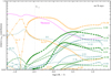 |
Fig. 10 Same as Fig. 9, but for the HD consistent model without any X-ray illumination. |
| In the text | |
Current usage metrics show cumulative count of Article Views (full-text article views including HTML views, PDF and ePub downloads, according to the available data) and Abstracts Views on Vision4Press platform.
Data correspond to usage on the plateform after 2015. The current usage metrics is available 48-96 hours after online publication and is updated daily on week days.
Initial download of the metrics may take a while.