| Issue |
A&A
Volume 609, January 2018
|
|
|---|---|---|
| Article Number | A50 | |
| Number of page(s) | 11 | |
| Section | Planets and planetary systems | |
| DOI | https://doi.org/10.1051/0004-6361/201731878 | |
| Published online | 05 January 2018 | |
Dust-driven viscous ring-instability in protoplanetary disks
Zentrum für Astronomie, Heidelberg University, Albert Ueberle Str. 2, 69120 Heidelberg, Germany
e-mail: dullemond@uni-heidelberg.de
Received: 1 September 2017
Accepted: 22 November 2017
Protoplanetary disks often appear as multiple concentric rings in dust continuum emission maps and scattered light images. These features are often associated with possible young planets in these disks. Many non-planetary explanations have also been suggested, including snow lines, dead zones and secular gravitational instabilities in the dust. In this paper we suggest another potential origin. The presence of copious amounts of dust tends to strongly reduce the conductivity of the gas, thereby inhibiting the magneto-rotational instability, and thus reducing the turbulence in the disk. From viscous disk theory it is known that a disk tends to increase its surface density in regions where the viscosity (i.e. turbulence) is low. Local maxima in the gas pressure tend to attract dust through radial drift, increasing the dust content even more. We have investigated mathematically if this could potentially lead to a feedback loop in which a perturbation in the dust surface density could perturb the gas surface density, leading to increased dust drift and thus amplification of the dust perturbation and, as a consequence, the gas perturbation. We find that this is indeed possible, even for moderately small dust grain sizes, which drift less efficiently, but which are more likely to affect the gas ionization degree. We speculate that this instability could be triggered by the small dust population initially, and when the local pressure maxima are strong enough, the larger dust grains get trapped and lead to the familiar ring-like shapes. We also discuss the many uncertainties and limitations of this model.
Key words: accretion, accretion disks / protoplanetary disks
© ESO, 2018
1. Introduction
High resolution, high contrast imaging at optical and sub-millimeter wavelengths has in recent years revealed that protoplanetary disks are highly structured. While some disks show complex non-axisymmetric structures, there are also numerous disks that display multiple nearly perfect concentric ringlike structures. The first and most prominent example was the disk around the star HL Tau (ALMA Partnership et al. 2015). Many other examples have since followed such as TW Hydra (Andrews et al. 2016; van Boekel et al. 2017), RX J1615.3 (de Boer et al. 2016), HD 97048 (Ginski et al. 2016), HD 163296 (Isella et al. 2016) and HD 169142 (Momose et al. 2015; Fedele et al. 2017). The rings are seen at submillimeter wavelength thermal dust emission as well as in optical/near-infrared scattered light. These rings and gaps have been interpreted as resulting from newly formed planets opening up gaps within the disk (e.g. Gonzalez et al. 2015; Kanagawa et al. 2015; Picogna & Kley 2015). This is an attractive scenario, because it would mean that we are indirectly “seeing” the young planets as they are being formed in their birth-disk. However, since we do not yet have direct indications of these planets, it is important to also investigate other explanations. Could these rings be caused by something entirely different altogether? And could this “something”, though unrelated to already existing planets, still teach us something about the formation of planets?
Various non-planet-related explanations for these rings have been proposed. In fact, their existence was predicted before their discovery, through a simple argument: It is known that dust aggregates of millimeter size and larger tend to radially drift toward the star on a very short time scale (Whipple 1972; Brauer et al. 2007). If the disk lives a few millions years, and the dust aggregates grow to the millimeter sizes inferred from millimeter-wave observations (e.g. Tazzari et al. 2016), then these disks should by the time they are observed already have lost most of their dust particles. By contrast, we see large quantities of dust in these disks, so something must be holding up the dust, preventing it from taking part in the rapid radial drift mechanism. It was suggested by Pinilla et al. (2012) that perhaps a multitude of local ring-shaped gas pressure bumps in the disk could trap the dust after it has grown to sizes of about a millimeter. The physical mechanism behind this dust trapping is the well-known, and unavoidable effect, that dust particles tend to drift toward regions of increased gas pressure (e.g. Whipple 1972; Adachi et al. 1976). Or in other words, that they drift in the direction of the gas pressure gradient ∇P. In smooth protoplanetary disks the gas pressure decreases with radius (∂rP< 0), which is the reason for the inward drift of dust. But if the gas pressure has wiggles that are strong enough that they cause ∂rP to flip sign, then there will exist local pressure maxima for which ∂rP = 0, and for which the dust drift is converging. In the absense of gas turbulence, all dust grains sufficiently close by would get trapped in these traps. Turbulence can mix the small dust grains (that are most strongly coupled to the gas) out of the traps, so that they may, on average, continue to drift inward. The bigger dust particles, which are less coupled to the gas, may still remain trapped. It depends on the amplitude of the pressure bumps and the strength of the turbulence, which grain sizes remain trapped and which not.
While the origin of these gas pressure bumps was not addressed in Pinilla et al. (2012), it was shown that if they exist, and if they are strong enough, the radial drift paradoxon could be solved. As a direct consequence, however, it was shown that high-resolution ALMA observations should then be able to see these dust rings, and the predicted ALMA images bear striking resemblance to HL Tau and similar sources.
This scenario does not, however, explain why these gas pressure bumps form in the first place. Takahashi & Inutsuka (2014, 2016) propose an elegant scenario in which dust rings are formed through a secular gravitational instability (Ward 2000). The idea is that if the dust density is high enough for a dust-driven gravitational instability to occur, the gas drag will slow this process down. The slowness of this process allows the information about the gravitational contraction to shear out and spread along azimuth, so that grand-design rings are formed instead of gravitationally contracting clumps. Takahashi & Inutsuka (2016) argue that as these rings contract further, this eventually leads to planets being formed, which, in their turn, open up gaps in the dust distribution (Paardekooper & Mellema 2004). They suggest that the ring-like structures could therefore be witnesses of both the initial and the final stages of planet formation.
A completely different scenario was proposed by Zhang et al. 2015, who argue that the locations of the rings suggest their association with the snow lines of a series of different volatile molecular species. A physical mechanism by which snow lines could lead to rings was worked out by Okuzumi et al. (2016). The physics of ice sublimation and deposition near these snow lines is complex, because it interacts strongly with the coagulation and fragmentation of dust aggregates, as well as with the radial drift and turbulent mixing in the disk (e.g. Stammler et al. 2017).
Gonzalez et al. (2017) propose an alternative scenario of spontaneous ring formation. In their model the radial drift of dust particles coupled to the dust coagulation process tends to lead to ring-like regions of high dust concentration and fast growth (see also Dra¸żkowska et al. 2016). While this might explain transition disks with a single dust ring, it may be more difficult to explain the multi-ring structures discussed here.
Global magnetohydrodynamical disk simulations with dead-zones also tend to create rings-shaped structures (Flock et al. 2015), and zonal flows (Johansen et al. 2009).
In this paper we investigate whether the viscous disk evolution could lead to the spontaneous formation of rings. This idea is not new. For instance, Wünsch et al. (2005) show, using 2D radiation-hydrodynamics models, that a disk with an active surface layer, self-gravity and “dead” midplane region could become viscously unstable and lead to the formation of several concentric rings. Our proposal is, however, based on a different physical driving mechanism. A version of this mechanism was already studied in a local box model by Johansen et al. (2011).
The ring instability works as follows. If we perturb an otherwise smooth disk with an infinitesimal-amplitude wiggle in the gas pressure (of the concentric ring type), it will tend to cause a slight enhancement of the dust-to-gas ratio in these pressure enhancements. This is the same physical mechanism as for dust trapping, but we do not necessarily need a flip of sign of ∂rP to cause this effect. It is just that the radial inward drift velocity | vdrift | of the dust is slightly increased on the outer side of the pressure enhancement and slightly reduced on the inner side, leading to a traffic-jam density enhancement effect. This effect works for big and small grains alike. It is known that dust has a negative influence on the disk viscosity, if it is caused by the magnetorotational instability (e.g. Sano et al. 2000; Ilgner & Nelson 2006; Okuzumi 2009; Dzyurkevich et al. 2013). A viscous disk reacts to the resulting wiggle in the viscosity ν(r) by adapting the surface density Σg(r) such that the steady-state  (1)is restored. So, whereever ν is reduced, Σg is increased. This change in Σg(r) amplifies the initial perturbation, resulting in a positive feedback loop. We therefore expect an initial perturbation in the gas disk to be amplified by the combined effect of dust drift and the effect the dust has on the viscosity of the disk. This process is depicted in cartoon form in Fig. 1.
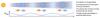 |
Fig. 1 Mechanism of the ring instability studied in this paper. |
To test whether this mechanism indeed works requires a linear perturbation analysis. This is what we present in this paper.
In Sect. 2 we give the basic equations that stand at the basis of our model. These are the standard viscous disk equations coupled to a single dust component of a given Stokes number.
The linear perturbation analysis of the combined gas and dust system is rather cumbersome. So in Sect. 3 we first simplify the system of equations radically, so that the mechanism presents itself more clearly. In Sect. 4 we then tackle the full set of equations, with some mathematics moved to the appendix.
2. Basic disk equations and model assumptions
The standard viscous disk equations for the gas together with a single dust component are: 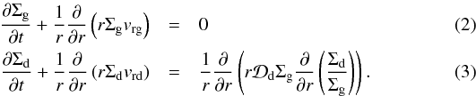 The gas radial velocity is given by the usual viscous disk equation:
  (4)with the turbulent viscosity defined by
  (5)where α is the usual alpha-turbulence parameter. The Kepler frequency is
  (6)with G the gravitational constant and M∗ the stellar mass. The isothermal sound speed squared is
  (7)with kB the Boltzmann constant, μ = 2.3 the mean molecular weight, and mp the proton mass. The vertical pressure scale height of the disk is
  (8)The dust diffusion constant is
  (9)where St is the Stokes number of the dust and Sc is the Schmidt number of the gas. The radial velocity of the dust is
  (10)where ρg is the midplane gas density and
  is the midplane gas pressure.
The α determines the strength of the turbulence, and hence the strength of the viscosity and the dust diffusivity. In our analysis we allow the dust surface density to affect the value of α: a higher dust concentration will lead to a lower α (e.g. Sano et al. 2000; Ilgner & Nelson 2006; Okuzumi 2009; Dzyurkevich et al. 2013). Since the physics of magnetorotational turbulence in non-ideal MHD is not yet fully understood, we parameterize this effect. We consider the following general prescription:  (11)where α1 is the unperturbed value of α, and likewise Σd1 and Σg1 are the unperturbed values of Σd and Σg respectively. The parameters φd and φg are powerlaw indices that parameterize how α depends on the change in dust and/or gas surface density. We focus on cases with φd< 0, meaning that an increase in Σd/ Σd1 leads to a decrease in α. The φg is used to allow for the following two cases of interest:
 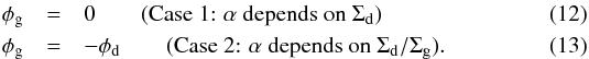 Case 1 could, at least in principle, allow for the expected instability even without dust drift relative to the gas, since without dust drift, Σd will necessarily increase if Σg does. In contrast, case 2 strictly requires dust drift for the instability to operate, since lack of dust drift keeps Σd/ Σg constant.
3. Simplified perturbation analysis
It is cumbersome to perform the linear stability analysis for the full set of equations of Sect. 2, because these equations contain factors  and the like. We postpone this full analysis to Sect. 4. For now, let us first simplify the equations.
3.1. Simplified equations
We simplify the equations to the following form: 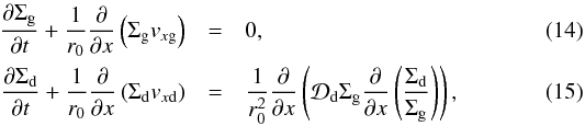 where r0 is the radius at which we wish to locally carry out the perturbation analysis, and x is the dimensionless radial coordinate starting from that location:
 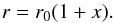 (16)The gas radial velocity formula (Eq. (4)) is simplified as:
 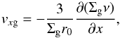 (17)with the viscosity still defined by Eq. (5). However, for simplicity cs and ΩK are now assumed be be constant. On the other hand, α is allowed to depend on x, but only due to the perturbation. The radial velocity of the dust is given, in our simplified description, by
  (18)The stationary solution is Σg = constant, Σd =constant and α =constant. This also yields vxd = vxg = 0 for that stationary solution. This stationary solution is the backdrop of our perturbation analysis.
Now we introduce an infinitesimal perturbation:  where Σg1 and Σd1 are the stationary (constant) solutions for gas and dust, respectively. From here on the subscript 1 denotes this stationary solution. We will also omit the (x,t) notation, to not clutter the equations too much. The symbols σg and σd are the dimensionless infinitesimal perturbations on the gas and the dust respectively. For the α, according to Eq. (11), we obtain, to leading order:
  (21)on account of the fact that | σd/g | ≪ 1.
Inserting these formulae into Eqs. (14), (15), and keeping in mind that both vxg and vxd are linear in the perturbations, and that we omit all terms of higher order in σg/d, we arrive, to leading order, at:  By inserting Eqs. (5), (19) together with Eqs. (21) into (17), and assuming that cs and ΩK are constant (see above), the radial velocity for the gas becomes
  (24)Similarly that of the dust becomes
  (25)Inserting these into the continuity equations (Eqs. (22), (23)) yields
  Now let us assume the linear perturbations to be plane waves in space x and time t. Since we seek modes for which the dust and the gas perturbations growth due to their mutual coupling, we can assume a single spatial frequency k and time frequency ω for both modes:
  The complex amplitudes A (for the gas) and B (for the dust) can be set independently. Inserting this mode into the above set of equations yields:
  where we made use of Eq. (9) to replace
  . This can be put into matrix form:
 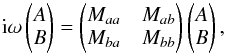 (32)with
  The eigenvalues of this matrix are found from:
  (37)So we have
  (38)The solution is stable if
  (39)for all possible values of k. One can see that if this is true/untrue for one value of k, it is true/untrue for all values of k, because k only enters as a multiplicative factor. The above stability condition requires that both Maa + Mbb< 0 and MaaMbb>MabMba. These two conditions simplify to:
 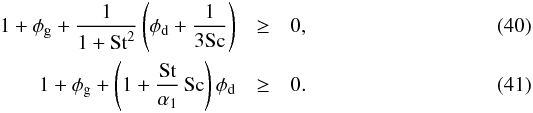 Both conditions have to be fulfilled for the disk to be stable against the dust-driven viscous instability. Otherwise it is unstable for all k.
3.2. Results for the growth rates
We apply the model to the case of a young solar mass star (M∗ = M⊙) with still substantial luminosity (L∗ = 10 L⊙), to mimic the case of HL Tau (ALMA Partnership et al. 2015). We perform the analysis at a radius of r0 = 60 au. The Schmidt number of the gas is set to Sc = 1. To compute the temperature of the midplane gas we assume a simple irradiated disk model, in which the irradiation angle is ϕ = 0.05. By setting the midplane temperature to the effective temperature of the disk assuming thermal equilibrium we obtain  , which is a very rough estimate of the disk temperature, but sufficient for the present purpose. The orbital time is 465 years. The vertical pressure scale height of the disk is Hp = cs/ ΩK = 6 au. We now apply the perturbation analysis for wave numbers k corresponding to dimensionless wavelengths λ = 2π/k in the range between the smallest possible wavelength λ = Hp/r0 and the largest reasonable one λ = 1. The choice of Hp/r0 is the smallest wavelength is based on the assumption that the turbulent viscosity in the disk cannot lead to radial structures that are narrower than about one vertical scale height. In the current example this means that the smallest wavelength we should consider is λ = 0.1.
We now compute the growth rate  (42)of each of these modes for a range of different dust particle sizes. We express the dust particle size in terms of its Stokes number St defined as St = tstop/torbit, where tstop is the stopping time of the dust particle defined as tstop = ffric/mgrain | vgrain−vgas | where ffric is the friction force between the gas and the dust particle, mgrain is the dust grain mass, and | vgrain−vgas | is the absolute value of the velocity difference between the gas and the dust particle. The precise translation between particle mass mgrain and Stokes number is not trivial to express, because it depends on much detailed physics, such as the porosity or fractility of the dust aggregate, its size compared to the gas mean free path, the gas density and temperature etc. For typical disk parameters a Stokes number of unity at 60 AU would correspond to a compact silicate dust particle of about a centimeter or a decimeter, and is smaller for smaller particles. We refer to the literature for an in-depth discussion of the relation between particle size and Stokes number (see e.g. Birnstiel et al. 2010). For our analysis only the Stokes number is relevant. The results of the present analysis are shown in Fig. 2.
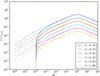 |
Fig. 2 Growth rate in units of the reciprocal orbital time (1 /torbit = ΩK/ 2π) of the dust-driven viscous instability, as a function of dust particle size (expressed as Stokes number St), according to the simplified analysis of Sect. 3. Dashed lines: case 1 (i.e. φg = 0), solid lines: case 2 (i.e. φg = −φd). The different lines show modes of different dimensionless wavelength λ in the dimensionless coordinate x, where λ = 2π/k. A dimensionless wavelength λ = 1 means a wavelength as large as r0. The parameters of the model shown here are φd = −1.0, α1 = 10-4, M∗ = 1 M⊙, L∗ = 10 L⊙, r0 = 60 au, T = 43,K, Sc = 1 (i.e. cs = 0.39 km s-1 and torbit = 465 yr). |
The growth rate Γ = Re(iω) is expressed in terms of the reciprocal orbital time scale. This means that if this value is larger than unity, the perturbation grows faster than the gas can orbit around the star. This would not lead to “grand-design” rings, but instead to small arc-shaped clumps, because if a perturbation is triggered at some azimuthal position, the information about this event does not have time to propagate around the entire orbit before the perturbation has grown to much larger amplitude. In other words: to create global-scale rings we need a slow instability (a “secular instability”). It must be slow compared to the time it takes for a perturbation to shear out over 2π in azimuth. This time scale depends on the radial width of the perturbation, which is related to the dimensionless wavelength λ of the unstable mode through Δr = r0λ. Through keplerian orbital dynamics we can then define this shear time scale as  (43)So instead of comparing Γ to the reciprocal orbital time, we should express Γ in terms of 1 /tshear. If we do so, the curves for small λ will move up. The results are shown in Fig. 3.
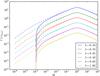 |
Fig. 3 Same as Fig. 2, but now with the growth rate Γ expressed in units of the reciprocal shear time over a radial distance of Δr = r0λ. |
Whereever the curve lies above unity, the growth is faster than the azimuthal communication. In that case small-scale arcs form instead of global scale rings. Wherever the curve lies sufficiently below unity but above zero (which in this log-representation means that the curve is visible in the plot), the perturbation may lead to large scale rings.
One can also see that, for case 2 (φg = −φd, solid lines in the figure) the instability does not operate for St ≤ 10-4 (for this set of model parameters), consistent with Eqs. (40), (41). This can be understood because for very small grains (small St) the dust is so well-coupled to the gas that dust drift is virtually inhibited, meaning that Σd/ Σg remains constant.
For both case 1 and case 2, however, the instability does not occur for St → 0, i.e. for the case in which the dust does not drift at all. This changes if we set φd< −1. In Fig. 4 the results for φd = −2 are shown (both case 1 and case 2). Now, at least for case 1 (φg = 0, dashed lines), the instability even operates for St → 0, i.e. without dust drift. The reason is that the convergent flow of gas, dragging along the dust with it, increases the gas and dust density enough to set the instability in motion. We then recover the instability by Hasegawa & Takeuchi (2015) and others. We discuss this in Sect. 5.
As can be seen, however, the strongest growth occurs around Stokes numbers of unity, and for the shortest wavelength λ. In this regime the growth rate is faster than 1 /tshear. In a disk with a grain size distribution spanning from tiny to large, this seems to suggest that the instability will be mainly driven by the comparetively large St ≃ 1 grains, which would then lead not to rings but to numerous small arcs. Perhaps these arcs can later merge into large scale rings is something that cannot be studied using this linear perturbation analysis.
In reality the situation is likely more subtle. In a disk with a dust size distribution it is typically the smallest grains that are affecting the α the most, because the smallest grains have the largest total surface area and can thus be most effective in removing free electrons and ions from the gas. We therefore speculate that in spite of the strong growth rate for St ≃ 1 particles that results from our analysis, it is mostly the smallest dust grains that drive the instability, if at all. If most/all of the dust has Stokes numbers below the cut-off for case 1, then if case 1 is applicable the instability would not operate at all.
3.3. A speculative scenario
Let us speculate about the following scenario: We assume that only relatively small dust affects the viscosity parameter α. From Fig. 3 for, say, St ≃ 3 × 10⁻⁴ the instability is driven at a low enough rate, even for the smallest wavelengths, that a set of global rings can form. As these rings grow in strength, we will enter into the non-linear regime. The radial derivative of the gas pressure will start to display sign-changes, and thus form actual dust traps. Since the disk also has large grains (even though they did not participate in the instability), these large grains get trapped into the dust traps and form dense dust rings, possibly even dominating the local density over the gas density. At this point the frictional back-reaction of the dust onto the gas will have to be taken into account, and the streaming instability (Johansen & Youdin 2007) may set in within these dust rings. Also the self-gravity of the population of large grains may start to play a role. Perhaps a combination with the secular instability of Takahashi & Inutsuka (2016) could occur. We are aware that these are mere speculations, and more investigation (in particular: numerical modeling) is required.
So far we have only looked at the growth rates of the modes, not their spatial propagation. In other words, we looked at Re(iω) but not yet at Im(iω). The above speculative scenario is only possible if the initial ring-instability occurs more or less in situ, or in other words, that it is not a moving wave that is slowly amplifying but instead a standing wave that is growing in amplitude. To verify this we need to study the ratio Im(iω)/Re(iω) for all cases where Re(iω) > 0. For the simplified analysis of this section it turns out that Im(iω) = 0. The mode grows exactly in-situ, meaning that the above speculative scenario is plausible.
4. Full perturbation analysis
The perturbation analysis for the full system of equations of Sect. 2 is substantially more tedious than the simplified analysis of Sect. 3, but the results are overall consistent with each other. There are also some simplifications that we keep: we still assume that the Stokes number does not change with time and space, and the same holds for the Schmidt number. In reality, for a given particle size the Stokes number changes if the gas density changes. Such effects are not included.
4.1. Stationary powerlaw solution
Let us assume the following Ansatz for the stationary solution: 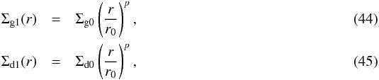 where we deliberately took the same powerlaw index for both the dust and the gas component. For the temperature profile we also assume a powerlaw of the form
 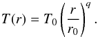 (46)The isothermal sound speed cs follows from this temperature by Eq. (7). The dimensionless vertical scale height h is defined as h = Hp/r, where the scale height Hp is given by Eq. (8).
The radial gas velocity (Eq. (4)) becomes  (47)where ν is given by Eq. (5). It can be aposteriori verified that stationary powerlaw solutions only exist if the α coefficient is independent of radius, which we will, from here on, assume to be the case. With Eq. (5) we then obtain
  (48)Inserting this into the gas continuity equation (Eq. (2)), and setting the time-derivative to zero, yields Σgν = constant. This means (with Eqs. (5), (6), (7), (46), (44)) that
  (49)Inserting this into Eq. (48) yields
  (50)Now let us do the dust, Eq. (3). Since by our Ansatz Σd(r)/Σg(r) is a constant (because both have the same powerlaw index), the right-hand-side of Eq. (3) is zero. This then immediately means that vd(r) /vg(r) must also be a constant. If we now look at the two terms in Eq. (10), and we assume that vd(r) must have the same radial powerlaw dependency as vg(r), then both terms in Eq. (10) must have the same radial powerlaw dependency. This means that csh must have the same radial powerlaw dependency on r as vrg:
  (51)where we used Eqs. (50), (5) and the definition of q (Eq. (46)) in the last step. However, given that
  we already independently know that
  (52)which confirms that we indeed have a stationary powerlaw solution for both the dust and the gas. We can now calculate the ratio of the dust radial velocity to the gas radial velocity using Eq. (10) with Eq. (44):
 ![\begin{eqnarray} \label{eq-vdust-vgas-stationary} \begin{split} v_{\rm rd} &= \frac{v_{\rm rg}}{1+\mathrm{St}^2} + \frac{c_{\rm s}h}{\mathrm{St}+\mathrm{St}^{-1}} \left(p + \frac{q-3}{2}\right)\\ &= \frac{1}{1+\mathrm{St}^2}\left[1+L\left(p+\frac{q-3}{2}\right)\right] \;v_{\rm rg}\comma \end{split} \end{eqnarray}](/articles/aa/full_html/2018/01/aa31878-17/aa31878-17-eq152.png) (53)where we define
(53)where we define  (54)where in the last step we used the stationary solution for vrg (Eq. (50)) and the equation for ν (Eq. (5)).
If we insert a standard example, p = −1, q = −0.5, then this becomes: ![\begin{equation} v_{\rm rd} = \frac{1}{1+\mathrm{St}^2}\left[1+1.833\,\frac{\mathrm{St}}{\alpha}\right] \;v_{\rm rg}\cdot \end{equation}](/articles/aa/full_html/2018/01/aa31878-17/aa31878-17-eq156.png) (55)
(55)
4.2. Linearization
Now we impose a perturbation on the stationary solution. We introduce the coordinate x:  (56)and the perturbations:
  similar to Sect. 3. Again, the subscript 1 denotes the stationary solution. We keep the temperature and sound speed stationary (i.e. static in time, but varying in space). The perturbations σd(x,t) and σg(x,t) are allowed to affect α(x,t). We use the same recipe for α as before (Eq. (11)). To first order in the perturbations we can write:
 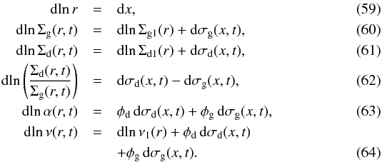 Or specifically for the double-logarithmic derivative with respect to r we obtain (omitting the (r,t) for notational convenience):
  The gas velocity vrg (Eq. (4)) is now:
  where we used Eqs. (69), (49). The dust velocity vrd (Eq. (10)) becomes, using Eqs. (6)–(8), (44), (65) and the identities h = Hp/r and
  :
: ![\begin{eqnarray} \label{eq-vdust-2} v_{\rm rd} &=& \frac{v_{\rm rg}}{1+\mathrm{St}^2} + \frac{c_{\rm s}h}{\mathrm{St}+\mathrm{St}^{-1}} \left(\frac{{\partial}{\ln}\,\Sigma_{\rm g}}{{\partial}{\ln}\,r} + \frac{q-3}{2}\right)\\ &=& \frac{v_{\rm rg}}{1+\mathrm{St}^2} \left[1+\frac{\mathrm{St}\,c_{\rm s}h}{v_{\rm rg}} \left(p+\frac{\partial \sigma_{\rm g}}{\partial x} + \frac{q-3}{2}\right)\right] \cdot\label{eq-vrdin-nu-with-perturb} \end{eqnarray}](/articles/aa/full_html/2018/01/aa31878-17/aa31878-17-eq168.png) To be able to use vrg and vrd in the viscous disk equations Eqs. (2), (3), will be forced to compute their radial derivatives, which is where the cumbersome math comes in. To keep things as orderly as possible, we rewrite Eqs. (2), (3) into double-logarithmic form:
To be able to use vrg and vrd in the viscous disk equations Eqs. (2), (3), will be forced to compute their radial derivatives, which is where the cumbersome math comes in. To keep things as orderly as possible, we rewrite Eqs. (2), (3) into double-logarithmic form:  The double-logarithmic derivatives of rΣg/dvr g/d can, using Eqs. (65), (66), be written out as
  (76)The right-hand-side of Eq. (75) can also be written into the derivatives of the perturbations. To first order in σg and σd we get:
  (77)where we made use of the fact that ∂(σd−σg) /∂x is already first order in σg and σd, and that
  is, to first order in σg and σd, constant. This is because the stationary solution (Sect. 4.1) obeys
  , which is constant.
What remains to be done is to derive expressions for the double-logarithmic derivatives of the gas and dust velocities (Eqs. (71) and (73), respectively) used in Eq. (76). This is somewhat tedious algebra, which we defer to Appendix A. After inserting the resulting expressions (Eqs. (A.3), (A.4)), into Eq. (76), we see that for both the gas and the dust version the constant term 1 + p drops out, and the expression of Eq. (76) becomes linear in the perturbations. This cancellation of the constant 1 + p is not surprising, because it follows from the fact that we start our perturbation analysis from the stationary solutions of Sect. 4.1. Inserting the resulting gas- and dust-versions of Eq. (76), together with Eq. (77), into the continuity equations Eqs. (74), (75), we find the following set of equations: ![\begin{eqnarray} \frac{\partial\sigma_{\rm g}}{\partial t} &+&\left[ \tilde C_{\rm g}\frac{\partial \sigma_{\rm g}}{\partial x} + \tilde C_{\rm gg}\frac{\partial^2\sigma_{\rm g}}{\partial x^2} + \tilde C_{\rm gd} \,\phi_{\rm d}\left( \frac{1}{2}\frac{\partial\sigma_{\rm d}}{\partial x} + \frac{\partial^2\sigma_{\rm d}}{\partial x^2}\right) \right. \nonumber\\ & & \left.+ \tilde C_{\rm gd} \,\phi_{\rm g}\left( \frac{1}{2}\frac{\partial\sigma_{\rm g}}{\partial x} + \frac{\partial^2\sigma_{\rm g}}{\partial x^2}\right) \right] = 0 \comma\label{eq-cont-gas-lin-2}\\ \frac{\partial\sigma_{\rm d}}{\partial t} &+&\left[ \tilde C_{\rm d}\frac{\partial \sigma_{\rm d}}{\partial x} + \tilde C_{\rm dg}\frac{\partial^2\sigma_{\rm g}}{\partial x^2} + \tilde C_{\rm dd} \,\phi_{\rm d}\left( \frac{1}{2}\frac{\partial\sigma_{\rm d}}{\partial x} + \frac{\partial^2\sigma_{\rm d}}{\partial x^2}\right) \right.\nonumber\\ & & \left. + \tilde C_{\rm dd} \,\phi_{\rm g}\left( \frac{1}{2}\frac{\partial\sigma_{\rm g}}{\partial x} + \frac{\partial^2\sigma_{\rm g}}{\partial x^2}\right) \right] = \tilde {\cal D}_{\rm d}\, \frac{\partial^2(\sigma_{\rm d}-\sigma_{\rm g})}{\partial x^2} \comma\label{eq-cont-dust-lin-2} \end{eqnarray}](/articles/aa/full_html/2018/01/aa31878-17/aa31878-17-eq177.png) where the tilde-symbols are defined as:
where the tilde-symbols are defined as:  where the symbols Cgg, Cgd, Cdg and Cdd are defined in Eqs. (A.5)–(A.8). We again insert trial functions
  and obtain the matrix equation (32)with
 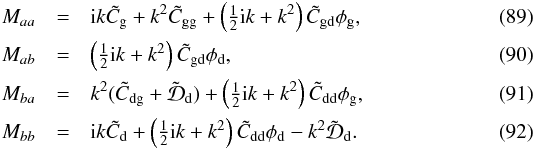 The eigenvalues, and thereby the growth rates of the modes, follow from Eqs. (37), (38).
4.3. Results
For the same parameters as in Sect. 3.2 we plot the resulting growth rates for the full perturbation analysis. The result is shown in Fig. 5 for case 2.
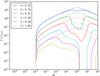 |
Fig. 5 Results for the full perturbation analysis of Sect. 4 (solid lines) compared to the results of the simplified perturbation analysis of Sect. 3 (dashed lines). Here case 2 is shown (φg = −φd) with φd = −1. For the rest the figure is the same as Fig. 3. If we would have plotted case 1 instead of case 2, the difference would only be that the curves would not be cut off for St ≲ 10-4, but would continue down to St → 0 in the same fashion as the dashed lines in Fig. 3. |
It shows that for small enough particles and small enough wavelength λ the simple perturbation analysis of Sect. 3 agrees well with the full perturbation analysis. The same is true if we would have plotted this diagram for case 1, the only difference to Fig. 5 being, that the curves would continue down to St → 0 as in Fig. 3. However, for larger particles and/or larger wavelength, the full perturbation analysis yields substantially weaker growth rates. But we see that for λ ≲ 0.25 the growth rates are nevertheless everywhere positive where the simplified analysis predicts positive growth rates. Since we need the instability to be slow to obtain large scale rings, this is, in fact, advantageous for the model.
As we did for the simplified analysis of Sect. 3.3 we have to verify if the initial ring-instability occurs more or less in situ. To this end we plot Im(iω)/Re(iω) (Fig. 6). We see that, in contrast to the simplified analysis, the imaginary component of iω is not zero. However, we see in the plot that for most Stokes numbers of interest Im(iω) is sufficiently much smaller than Re(iω). That means that the growth can be considered to be sufficiently well in situ for the speculative scenario of Sect. 3.3 to remain plausible.
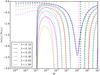 |
Fig. 6 Ratio of Im(iω)/Re(iω) for the full perturbation analysis. Dashed lines: case 1 (φd = −1, φg = 0), solid lines: case 2 (φd = −1, φg = 1). |
5. Discussion
5.1. Limitations and speculations
The linear stability analysis of this paper shows that, at least in principle, the combination of viscous disk theory, radial drift of dust, and the negative feedback of the dust on the viscosity, could lead to ring-shaped patterns in a protoplanetary disk.
The linear growth rate depends on the size of the dust grains, or more precisely: on their Stokes number. Depending on the prescription of the feedback, the instability is inhibited for the very small Stokes numbers. But for Stokes numbers beyond a critical value, the growth rate increases with increasing St. Around St ≃ 1 the instability is suppressed again. Figure 5 shows the growth rates as a function of St for given wavelengths of the mode.
Not surprisingly, the instability grows the quickest for the shortest wavelengths. The shortest wavelength is expected to be the disk pressure scale height, which is therefore expected to be the dominant mode.
However, the feedback of the dust onto the viscosity of the gas is a surface-area effect (dust grains removing free electrons and ions from the gas), so one should expect the feedback to be the strongest for the smallest grains. In our model we did not include this effect: we took the same feedback recipe (Eq. (11)) independent on grain size. We speculate that if a disk contains a size distribution of dust, the smallest grains with Stokes numbers still beyond the critical one, will be the ones that drive the instability. Since the growth rate of the instability for such grain sizes is substantially slower than the time a blob would be sheared out into a ring (see Fig. 5), the information about the growth of the instability can be communicated over the full 2π azimuth of the disk, so that a global ring is formed instead of a set of independent arcs.
With our model we cannot study what happens if the instability becomes non-linear. Assuming we have a size distribution of dust grains, then, although only the smaller grains drive the instability, also the larger grains will undergo density enhancements: they will do so even stronger than the instability-driving smaller grains. Once the mode becomes so strong that rings of positive pressure gradient are produced, then the larger grains will get trapped. Turbulent mixing always leaks a few of these grains out of the traps, but on the whole, large grains would be trapped and produce large-amplitude rings made from millimeter to centimeter size grains, similar to what is seen with ALMA in many sources. Our perturbation analysis suggests that the shortest wavelengths grow the quickest. However, viscous disk theory works on scales equal to or larger than the pressure scale height. The spacing between the rings in the gas structure of the disk will therefore be at least a pressure scale height. The large dust grains, however, could conceivably get trapped in rings that are thinner than that.
In this two-stage scenario (small grains triggering the rings, large grains getting trapped) the rings have to be sustained. If the small grains coagulate and become large, their ability to affect α reduces, and the rings may dissipate. Maybe this can be prevented through a bit of fragmentation of the pebbles, producing fresh fine grained dust. Even for low levels of turbulence the collision velocities of the pebbles may be relatively high. The typical turbulent eddy velocity at the top of the Kolmogorov cascade is  . With a temperature of, say, 100 K one has cs = 0.6 km s-1. If the fragmentation velocity is 1 m/s (e.g. Güttler et al. 2010) one would need α ≲ 3 × 10⁻⁶ to prevent fragmentation. Anything above that would lead to the production of small grains. It is therefore feasible that a sufficient amount of small grains are continuously regenerated to keep the rings in place. On the other hand, aggregates made up of icy grains are thought to be more robust, and may fragment only at collision velocities of ~ 10 m/s, or even up to ~50 m/s, depending on the size of the monomers of which they are made (Wada et al. 2009)
Dust aggregates are most likely porous or fractal. Large “pebbles” may therefore still have rather large surface-to-mass ratios, and thus still strongly affect the ionization degree of the disk. We would, however, also observe them as if they were much smaller than they are, since also the optical properties of such dust aggregates depend a lot on the surface-to-mass ratio (Kataoka et al. 2014). The “big grains” that we identify as “big” due to their opacity slope at millimeter wavelengths therefore presumably also have a relatively low surface-to-mass ratio, and thus have little influence on the ionization degree of the disk. To have such big grains arranged in rings, we really need this two-stage scenario, as the big grains cannot (according to our scenario) generate the rings themselves.
There is, however, a big uncertainty with the model: the role of the vertical structure. Small grains can be turbulently stirred to several pressure scale heights above the midplane, even for relatively low turbulent α. Is it therefore still justified to assume that the wavelength of one pressure scale height to be the strongest growing mode? Could it be that this would lead to sufficient radial smearing that larger wavelength modes dominate? Okuzumi & Hirose (2011) study the effect of the vertical structure on the viscosity of the disk. They conclude that the vertically averaged magneto-turbulent viscosity only depends on the resistivity profile (and thereby on the vertically averaged dust abundance) through three critical heights, and is largely insensitive to the details of the resistivity profile itself. This may mean that the vertically averaged dust abundance has, in most parts of the disk, only limited influence (S. Okuzumi, priv. comm.).
Multi-wavelength observations of the same sources can help answer these questions. For instance, for TW Hydra both millimeter (Andrews et al. 2016) and H-band observations (van Boekel et al. 2017) exist. van Boekel et al. (2017) study how the rings in the millimeter compare to the large scale rings in the H-band. Some correspondence is found, but overall the structures appear to be uncorrelated, which appears to argue against our model, at least for this source.
5.2. On rings and the slowness of the instability
As argued in this paper, for an instability to lead to ring-like structures rather than patchy/clumpy structures in a disk, the instability has to be slower than the shear. This is the case for the dust-driven viscous instability discussed in this paper. In hindsight this is not surprising, since the viscous time scale of the disk can be quite long. One can quantify this by considering a perturbation with radial width W (i.e. in our dimensionless form this is W = λr). If we express W in units of the pressure scale height, which is the narrowest viscous structures we can expect in the disk, we get 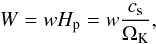 (93)The viscous time scale for this perturbation is
 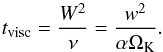 (94)The shear time (from Eq. (43)) is
  (95)The condition for the instability to be slow enough then becomes
  (96)The smallest possible value for w is 1, which is also the fastest growing mode. This shows that if α is much smaller than the disk’s dimensionless thickness (aspect ratio), then the instability (if it exists) is slow enough to create rings instead of patches. For a typical disk Hp/r ≃ 0.05···0.1 this means that α ≪ 10-2 for the instability to be slow enough. Therefore we can conclude that, if the rings seen in numerous disks are due to any form of viscous instability, the viscosity of the disk must be substantially lower than the canonical value of 10-2, or the instability must be slowed down by an even slower process such as dust drift of small enough dust grains.
5.3. Comparison to earlier work
The ring-instability we have investigated in this paper appears to have a relation to the ring-instability found by Wünsch et al. (2005). In their model the disk had an active surface layer and a passive (“dead”) midplane layer. If gas would accumulate at some radius, the surface density of the active layer stays the same, but that of the dead layer increases. In a vertically averaged sense the viscosity thus gets reduced. This is mathematically identical to our case of φd = −1 and φg = 0 (prescription 1, Eqs. (11), (12)), with St = 0. In our model, however, we do not find an instability for these parameters. However, Wünsch et al. (2005) include the effect of the perturbation on the disk midplane temperature, which we do not. In our case we indeed get the instability if φd< −1.
Hasegawa & Takeuchi (2015) also studied the behavior of the two-layered disk model. They find that if the effective α of the two-layered disk is simply an average of the active and dead layers (weighted by their respective surface densities), then the disk remains stable. Our model with φd = −1 and φg = 0 (prescription 1) and St = 0 (no dust drift) confirms this. When they apply a more sophisticated effective α recipe, based on Okuzumi & Hirose (2011), they find that the disk becomes unstable near the dead zone outer edge, because that is where the dependence of α on Σ is the steepest. Our model confirms this, because the more sophisticated α recipe has a steeper dependence of α on Σ, which would amount, in our work, to φd< −1 (again taking φg = 0 and St = 0), which we confirm to lead to instability. Our model is thus consistent with the earlier work by Hasegawa & Takeuchi (2015). But by including dust drift our model is more general.
Flock et al. (2015) perform 3D full disk non-ideal MHD models and find ringlike structures, too, although rather wide ones and only two of them. But like Hasegawa & Takeuchi (2015), this is unrelated to dust drift.
Our dust-drift induced viscous instability is, however, very similar to the instability found by Johansen et al. (2011). While the analysis in that paper is locally more detailed (including radial and azimuthal motions), our linear stability analysis includes the radial gradients and the global cylindrical geometry terms an is thus not just a local analysis. Furthermore our analysis includes the radial drift, as well as the turbulent diffusion, both of which play a key role in the mechanism. Moreover, we argue that the slowness of the instability is critical in getting grand-design rings rather than chaotic arc-shaped structures.
The analysis in this paper is by no means a proof of the feasibility of this scenario. It will require detailed 2D/3D viscous hydrodynamic disk modeling, and comparisons to observations, to test this scenario.
6. Conclusion
In this paper we show that it is conceivable that the combination of viscous disk theory, radial drift of dust, and the negative feedback of the dust on the viscosity, can produce (or at least trigger the formation of) ring-shaped patterns in protoplanetary disks similar to what is seen in protoplanetary disks at millimeter and optical/near-infrared wavelengths. From our present analysis we conclude:
-
1.
Even without dust drift, if ∂ln α/∂ln Σ < −1, the disk is prone to the viscous ringinstability. This is a conclusion in agreement with work byHasegawa & Takeuchi (2015).
-
2.
When dust grains are large enough to start drifting, yet small enough to have a substantial influence on the viscosity of the disk (through their ability to capture free electrons and ions from the gas), dust drift tends to cause a feedback loop on the disk viscosity, leading to dust-rich regions of low viscosity and dust-poor regions of high viscosity. In this way dust drift can trigger the viscous instability even when the disk would be stable otherwise (∂ln α/∂ln Σ ≥ −1). These findings are consistent with Johansen et al. (2011), and generalize them to global disk accretion with generalized viscosity description.
-
3.
The radial drift due to the global pressure gradient in the disk does not suppress the instability for small grains, but does so for grains with Stokes number near unity. The ring instability (viscous instability) must therefore be driven by small enough grains. This also agrees with the issue that small grains more easily affect the viscosity of the disk, because due to their larger surface-to-mass ratio, they more easily capture free electrons and ions.
-
4.
For grand-design rings to form, such as those observed in real protoplanetary disks, rather than pseudo-random patchy structures, the growth rate of the instability must be slower than the shear-out time scale. Our analysis shows that this is generally the case, if the instability is driven by small enough grains and/or if the viscous α ≪ 10-2.
-
5.
If the grains are too small, they hardly drift. Whether the disk is then stable or not depends strongly on the viscosity recipe. We have identified two cases: case 1 in which the absolute value of the dust density determines the viscous α and case 2 in which the ratio of dust-to-gas density determines the viscous α. For very small grains, the disk becomes stable for case 2, but may still become unstable for case 1, if the dependence of α on 1/Σ is steep enough.
-
6.
Observations seem to show that the rings seen at millimeter wavelengths are populated by relatively large rains. Since the viscous ring instability seems to be driven by small grains, this may seem inconsistent at first. We suggest that the initial rings are created by the viscous instability, which then produces strong enough dust traps that the larger grains get trapped and produce the ALMA images observed.
Acknowledgments
This research was supported by the Munich Institute for Astro- and Particle Physics (MIAPP) of the DFG cluster of excellence “Origin and Structure of the Universe”. We thank Satoshi Okuzumi for interesting discussions regarding the effect of the vertical structure. We thank the anonymous referee for insightful comments which helped improve the manuscript.
References
- Adachi, I., Hayashi, C., & Nakazawa, K. 1976, Prog. Theor. Phys., 56, 1756 [NASA ADS] [CrossRef] [Google Scholar]
- ALMA Partnership, Brogan, C. L., Pérez, L. M., et al. 2015, ApJ, 808, L3 [NASA ADS] [CrossRef] [Google Scholar]
- Andrews, S. M., Wilner, D. J., Zhu, Z., et al. 2016, ApJ, 820, L40 [NASA ADS] [CrossRef] [Google Scholar]
- Birnstiel, T., Dullemond, C. P., & Brauer, F. 2010, A&A, 513, A79 [NASA ADS] [CrossRef] [EDP Sciences] [Google Scholar]
- Brauer, F., Dullemond, C. P., Johansen, A., et al. 2007, A&A, 469, 1169 [NASA ADS] [CrossRef] [EDP Sciences] [Google Scholar]
- de Boer, J., Salter, G., Benisty, M., et al. 2016, A&A, 595, A114 [NASA ADS] [CrossRef] [EDP Sciences] [Google Scholar]
- Drążkowska, J., Alibert, Y., & Moore, B. 2016, A&A, 594, A105 [NASA ADS] [CrossRef] [EDP Sciences] [Google Scholar]
- Dzyurkevich, N., Turner, N. J., Henning, T., & Kley, W. 2013, ApJ, 765, 114 [NASA ADS] [CrossRef] [Google Scholar]
- Fedele, D., Carney, M., Hogerheijde, M. R., et al. 2017, A&A, 600, A72 [NASA ADS] [CrossRef] [EDP Sciences] [Google Scholar]
- Flock, M., Ruge, J. P., Dzyurkevich, N., et al. 2015, A&A, 574, A68 [NASA ADS] [CrossRef] [EDP Sciences] [Google Scholar]
- Ginski, C., Stolker, T., Pinilla, P., et al. 2016, A&A, 595, A112 [NASA ADS] [CrossRef] [EDP Sciences] [Google Scholar]
- Gonzalez, J.-F., Laibe, G., Maddison, S. T., Pinte, C., & Ménard, F. 2015, MNRAS, 454, L36 [NASA ADS] [CrossRef] [Google Scholar]
- Gonzalez, J.-F., Laibe, G., & Maddison, S. T. 2017, MNRAS, 467, 1984 [NASA ADS] [Google Scholar]
- Güttler, C., Blum, J., Zsom, A., Ormel, C. W., & Dullemond, C. P. 2010, A&A, 513, A56 [NASA ADS] [CrossRef] [EDP Sciences] [Google Scholar]
- Hasegawa, Y., & Takeuchi, T. 2015, ApJ, 815, 99 [NASA ADS] [CrossRef] [Google Scholar]
- Ilgner, M., & Nelson, R. P. 2006, A&A, 445, 205 [NASA ADS] [CrossRef] [EDP Sciences] [Google Scholar]
- Isella, A., Guidi, G., Testi, L., et al. 2016, Phys. Rev. Lett., 117, 251101 [NASA ADS] [CrossRef] [Google Scholar]
- Johansen, A., & Youdin, A. 2007, ApJ, 662, 627 [NASA ADS] [CrossRef] [Google Scholar]
- Johansen, A., Youdin, A., & Klahr, H. 2009, ApJ, 697, 1269 [NASA ADS] [CrossRef] [Google Scholar]
- Johansen, A., Kato, M., & Sano, T. 2011, in Advances in Plasma Astrophysics, eds. A. Bonanno, E. de Gouveia Dal Pino, & A. G. Kosovichev, IAU Symp., 274, 50 [Google Scholar]
- Kanagawa, K. D., Muto, T., Tanaka, H., et al. 2015, ApJ, 806, L15 [NASA ADS] [CrossRef] [Google Scholar]
- Kataoka, A., Okuzumi, S., Tanaka, H., & Nomura, H. 2014, A&A, 568, A42 [NASA ADS] [CrossRef] [EDP Sciences] [Google Scholar]
- Momose, M., Morita, A., Fukagawa, M., et al. 2015, PASJ, 67, 83 [NASA ADS] [CrossRef] [Google Scholar]
- Okuzumi, S. 2009, ApJ, 698, 1122 [NASA ADS] [CrossRef] [Google Scholar]
- Okuzumi, S., & Hirose, S. 2011, ApJ, 742, 65 [NASA ADS] [CrossRef] [Google Scholar]
- Okuzumi, S., Momose, M., Sirono, S.-I., Kobayashi, H., & Tanaka, H. 2016, ApJ, 821, 82 [NASA ADS] [CrossRef] [Google Scholar]
- Paardekooper, S.-J., & Mellema, G. 2004, A&A, 425, L9 [NASA ADS] [CrossRef] [EDP Sciences] [Google Scholar]
- Picogna, G., & Kley, W. 2015, A&A, 584, A110 [NASA ADS] [CrossRef] [EDP Sciences] [Google Scholar]
- Pinilla, P., Birnstiel, T., Ricci, L., et al. 2012, A&A, 538, A114 [NASA ADS] [CrossRef] [EDP Sciences] [Google Scholar]
- Sano, T., Miyama, S. M., Umebayashi, T., & Nakano, T. 2000, ApJ, 543, 486 [NASA ADS] [CrossRef] [Google Scholar]
- Stammler, S. M., Birnstiel, T., Panić, O., Dullemond, C. P., & Dominik, C. 2017, A&A, 600, A140 [NASA ADS] [CrossRef] [EDP Sciences] [Google Scholar]
- Takahashi, S. Z., & Inutsuka, S.-I. 2014, ApJ, 794, 55 [NASA ADS] [CrossRef] [Google Scholar]
- Takahashi, S. Z., & Inutsuka, S.-I. 2016, AJ, 152, 184 [NASA ADS] [CrossRef] [Google Scholar]
- Tazzari, M., Testi, L., Ercolano, B., et al. 2016, A&A, 588, A53 [NASA ADS] [CrossRef] [EDP Sciences] [Google Scholar]
- van Boekel, R., Henning, T., Menu, J., et al. 2017, ApJ, 837, 132 [NASA ADS] [CrossRef] [Google Scholar]
- Wada, K., Tanaka, H., Suyama, T., Kimura, H., & Yamamoto, T. 2009, ApJ, 702, 1490 [NASA ADS] [CrossRef] [Google Scholar]
- Ward, W. R. 2000, On Planetesimal Formation: the Role of Collective Particle Behavior, eds. R. M. Canup, & K. Righter (Tucson: University of Arizona Press), 75 [Google Scholar]
- Whipple, F. L. 1972, in From Plasma to Planet, ed. A. Elvius, 211 [Google Scholar]
- Wünsch, R., Klahr, H., & Różyczka, M. 2005, MNRAS, 362, 361 [NASA ADS] [CrossRef] [Google Scholar]
- Zhang, K., Blake, G. A., & Bergin, E. A. 2015, ApJ, 806, L7 [NASA ADS] [CrossRef] [Google Scholar]
Appendix A: Double-logarithmic derivatives of the velocities
The double-logarithmic derivative of the gas velocity with respect to r is computed from Eq. (71) by initially taking the single-logarithmic-derivative ∂vrg/∂ln r, working out ∂(ν/r)∂ln r, and dividing again by Eq. (71), where one regularly makes use of the fact that | σg/d | ≪ 1 and that we expand only to first order in σg/d.
For the double-logarithmic derivative of the dust velocity with respect to r we start from Eq. (73), and make use of the result we already obtained for the double-logarithmic derivative of vrg. Again we regularly make use of the fact that | σg/d | ≪ 1 and that we expand only to first order in σg/d. To make the algebra more convenient we define 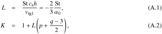 where Eq. (A.1) is, in fact, the same as Eq. (54).
After substantial algebra we find: ![\appendix \setcounter{section}{1} \begin{eqnarray} \frac{{\partial}{\ln} |v_{\rm rg}|}{{\partial}{\ln}\, r} &=&-(p+1) + C_{\rm gg}\frac{\partial^2\sigma_{\rm g}}{\partial x^2}\nonumber\\[2mm] &&+C_{\rm gd}\phi_{\rm d}\left( \frac{1}{2}\frac{\partial\sigma_{\rm d}}{\partial x} + \frac{\partial^2\sigma_{\rm d}}{\partial x^2}\right)\nonumber\\[2mm] &&+C_{\rm gd}\phi_{\rm g}\left( \frac{1}{2}\frac{\partial\sigma_{\rm g}}{\partial x} + \frac{\partial^2\sigma_{\rm g}}{\partial x^2}\right)\comma\label{eq-dbllog-lin-der-vrg-2}\\[2mm] \frac{{\partial}{\ln} |v_{\rm rd}|}{{\partial}{\ln}\, r} &=&-(p+1) + C_{\rm dg}\frac{\partial^2\sigma_{\rm g}}{\partial x^2}\nonumber\\[2mm] &&+C_{\rm dd}\phi_{\rm d}\left( \frac{1}{2}\frac{\partial\sigma_{\rm d}}{\partial x} + \frac{\partial^2\sigma_{\rm d}}{\partial x^2}\right)\nonumber\\[2mm] &&+C_{\rm dd}\phi_{\rm g}\left( \frac{1}{2}\frac{\partial\sigma_{\rm g}}{\partial x} + \frac{\partial^2\sigma_{\rm g}}{\partial x^2}\right)\comma\label{eq-dbllog-lin-der-vrd-2} \end{eqnarray}](/articles/aa/full_html/2018/01/aa31878-17/aa31878-17-eq215.png) with
with ![\appendix \setcounter{section}{1} \begin{eqnarray} C_{\rm gg} &=& 2\comma\label{eq-define-cgg}\\[2mm] C_{\rm gd} &=& 2\comma\label{eq-define-cgd}\\[2mm] C_{\rm dg} &=&2\left[1-\frac{L}{K}\left(p+\frac{q-4}{2}\right)\right] = \frac{12-4\,\mathrm{St}/\alpha_0}{6+11\,\mathrm{St}/\alpha_0}\comma\label{eq-define-cdg}\\[2mm] C_{\rm dd} &=&2\left[1-\frac{L}{K}\left(p+\frac{q-3}{2}\right)\right] = \frac{12}{6+11\,\mathrm{St}/\alpha_0}\label{eq-define-cdd}\cdot \end{eqnarray}](/articles/aa/full_html/2018/01/aa31878-17/aa31878-17-eq216.png) The second identities in Eqs. (A.7), (A.8) are for the case p = −1, q = −1/2.
The second identities in Eqs. (A.7), (A.8) are for the case p = −1, q = −1/2.
All Figures
|
Fig. 1 Mechanism of the ring instability studied in this paper. |
| In the text | |
|
Fig. 2 Growth rate in units of the reciprocal orbital time (1 /torbit = ΩK/ 2π) of the dust-driven viscous instability, as a function of dust particle size (expressed as Stokes number St), according to the simplified analysis of Sect. 3. Dashed lines: case 1 (i.e. φg = 0), solid lines: case 2 (i.e. φg = −φd). The different lines show modes of different dimensionless wavelength λ in the dimensionless coordinate x, where λ = 2π/k. A dimensionless wavelength λ = 1 means a wavelength as large as r0. The parameters of the model shown here are φd = −1.0, α1 = 10-4, M∗ = 1 M⊙, L∗ = 10 L⊙, r0 = 60 au, T = 43,K, Sc = 1 (i.e. cs = 0.39 km s-1 and torbit = 465 yr). |
| In the text | |
|
Fig. 3 Same as Fig. 2, but now with the growth rate Γ expressed in units of the reciprocal shear time over a radial distance of Δr = r0λ. |
| In the text | |
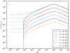 |
Fig. 4 Same as Fig. 3, but now for φd = −2 instead of φd = −1. |
| In the text | |
|
Fig. 5 Results for the full perturbation analysis of Sect. 4 (solid lines) compared to the results of the simplified perturbation analysis of Sect. 3 (dashed lines). Here case 2 is shown (φg = −φd) with φd = −1. For the rest the figure is the same as Fig. 3. If we would have plotted case 1 instead of case 2, the difference would only be that the curves would not be cut off for St ≲ 10-4, but would continue down to St → 0 in the same fashion as the dashed lines in Fig. 3. |
| In the text | |
|
Fig. 6 Ratio of Im(iω)/Re(iω) for the full perturbation analysis. Dashed lines: case 1 (φd = −1, φg = 0), solid lines: case 2 (φd = −1, φg = 1). |
| In the text | |
Current usage metrics show cumulative count of Article Views (full-text article views including HTML views, PDF and ePub downloads, according to the available data) and Abstracts Views on Vision4Press platform.
Data correspond to usage on the plateform after 2015. The current usage metrics is available 48-96 hours after online publication and is updated daily on week days.
Initial download of the metrics may take a while.