| Issue |
A&A
Volume 609, January 2018
|
|
|---|---|---|
| Article Number | A126 | |
| Number of page(s) | 24 | |
| Section | Interstellar and circumstellar matter | |
| DOI | https://doi.org/10.1051/0004-6361/201731788 | |
| Published online | 01 February 2018 | |
Expansion patterns and parallaxes for planetary nebulae ⋆
1 Leibniz-Institut für Astrophysik Potsdam (AIP), An der Sternwarte 16, 14482 Potsdam, Germany
e-mail: This email address is being protected from spambots. You need JavaScript enabled to view it.
2 Astronomy Department, University of Washington, Seattle, WA 98195, USA
e-mail: This email address is being protected from spambots. You need JavaScript enabled to view it.
Received: 17 August 2017
Accepted: 25 September 2017
Abstract
Aims. We aim to determine individual distances to a small number of rather round, quite regularly shaped planetary nebulae by combining their angular expansion in the plane of the sky with a spectroscopically measured expansion along the line of sight.
Methods. We combined up to three epochs of Hubble Space Telescope imaging data and determined the angular proper motions of rim and shell edges and of other features. These results are combined with measured expansion speeds to determine individual distances by assuming that line of sight and sky-plane expansions are equal. We employed 1D radiation-hydrodynamics simulations of nebular evolution to correct for the difference between the spectroscopically measured expansion velocities of rim and shell and of their respective shock fronts.
Results. Rim and shell are two independently expanding entities, driven by different physical mechanisms, although their model-based expansion timescales are quite similar. We derive good individual distances for 15 objects, and the main results are as follows: (i) distances derived from rim and shell agree well; (ii) comparison with the statistical distances in the literature gives reasonable agreement; (iii) our distances disagree with those derived by spectroscopic methods; (iv) central-star “plateau” luminosities range from about 2000 L⊙ to well below 10 000 L⊙, with a mean value at about 5000 L⊙, in excellent agreement with other samples of known distance (Galactic bulge, Magellanic Clouds, and K648 in the globular cluster M 15); (v) the central-star mass range is rather restricted: from about 0.53 to about 0.56 M⊙, with a mean value of 0.55 M⊙.
Conclusions. The expansion measurements of nebular rim and shell edges confirm the predictions of radiation-hydrodynamics simulations and offer a reliable method for the evaluation of distances to suited objects.
Key words: planetary nebulae: general / stars: fundamental parameters / techniques: image processing / techniques: spectroscopic
Results of this paper are based on observations made with the NASA/ESA Hubble Space Telescope in Cycle 16 (GO11122) and older data obtained from the Data Archive at the Space Telescope Science Institute, which is operated by the Association of Universities for Research in Astronomy, Inc., under NASA contract NAS 5-26555.
© ESO, 2018
1. Introduction
For many years long-slit Doppler studies of planetary nebulae (PNe) have shown that structures in PNe expand at mildly supersonic speeds of order 10−30 km s-1 or more (see compilations by Hajian et al. 2007; López et al. 2012; Schönberner et al. 2014). Their speeds and sharp leading edges argue that the expansions are actually pressure-driven. In general, these velocities correspond to proper motions of 0.̋02 to over 0.̋06 in a decade at a distance of 1 kpc. Therefore the expansion patterns of PNe with simple, sharp-edged features can discerned in repeated high-spatial-resolution images that span a decade using geometrically stable cameras (Liller 1965; Liller et al. 1966; Osterbrock 1966; Hajian et al. 1995). As these papers highlight, the Doppler expansion speeds divided by the corresponding angular expansion rates can, in principle, be combined to derive distances to PNe using the “expansion parallax method”. Once their distances are known, many intrinsic properties of the PNe and their central stars (mass, luminosity, death rates, Galactic distribution) are derivable. For the bulk of objects one has, however, to rely on statistical distance scales that depend on poorly justified assumptions. Accordingly, objects with known parallax serve as excellent calibrators.
A comprehensive discussion of commonly used methods to obtain individual distances for PNe can be found in Frew (2008). Based on individual distances of about 120 calibrating sources, a new distance scale was devised which is based on the Hα-surface brightness evolution with nebular radius. The reliability of this distance calibration has been supported recently by Jacob et al. (2013) by employing radiation-hydrodynamics models. An update of Frew’s 2008 calibration is given in Frew et al. (2016).
Individual distances of higher accuracy are urgently needed since they enable estimates of masses via the (core) mass-luminosity relation for post-asymptotic-giant-branch (post-AGB) stars. This mass can be compared with the mass that follows from distance-independent methods, for example, from detailed spectroscopic determinations of the photospheric parameters by non-LTE model atmospheres and comparison with evolutionary tracks in the log g-Teff plane or from sophisticated radiation-hydrodynamical wind models which provide stellar mass, radius, and luminosity without referring to any stellar model calculations.
However, radiation-hydrodynamical models of Pauldrach et al. (2004) argued that (i) the dependence of stellar luminosity with mass is smaller than expected and (ii) the central stars of some well-studied PN had luminosities 4.2 < log (L/L⊙) < 4.5 and masses right at the Chandrasaekhar limit. The reliability of their wind models have been reinforced by Kaschinski et al. (2012) and Hoffmann et al. (2016). Because of this quite disturbing finding any independent determination of the distance to the objects in question would be of utmost relevance not only for accurate determinations of stellar properties but also for checking the complicated physics underlying stellar wind models.
The Hubble Space Telescope (HST) and large radio interferometers with subarcsecond resolution have revolutionized expansion studies. Expansions and proper motions are best derived from geometrically simple PNe with bright, sharp-edged features with angular diameters of 30′′ or less. Systematic radial expansion patterns have been monitored from multi-epoch HST images for NGC 6543 (Reed et al. 1999; Balick & Hajian 2004), BD + 30°3639 (Akras & Steffen 2012; Li et al. 2002) and a few other PNe (Palen et al. 2002; Hajian et al. 1995). Similar expansions have also been found from radio images using the Very Large Array (VLA) for NGC 7027 (Zijlstra et al. 2008), M2-42 Guzmán et al. (2006), IC 418 (Guzmán et al. 2009), and NGC 6881 (Guzmán-Ramírez et al. 2011).
In this paper, we present HST/WFPC2 images of a dozen additional bright PNe with simple geometries in the emission lines of Hα, [O iii], and [N iii] to: (1) more generally characterize the rates and patterns of the expansions of PNe, and (2) extend the measurements of expansion distances to another dozen bright targets with relatively simple shapes and sharp-edged features.
The application of radiation-hydrodynamical models to high-quality multi-epoch HST images for the derivation of accurate distances is the primary contribution of this paper. As we shall see, the outer edge of a smooth shell is the simplest means to measure expansion distances. However, it is much fainter then the bright rim of the cavity inside, so its position is more poorly defined. On the other hand, the bright rim is generally a bubble-driven shock, a pattern that moves through the gas at a speed that may not represent that of the gas inside it. Where possible we measure the expansion rates of both features and use our models to convert the shock pattern motions into true gas motions.
This paper is organised as follows: in Sect. 2 we present details of the observations and the selection of suited objects for a detailed analysis. In Sect. 3, we determine and compare the apparent expansions of nebular edges (rims, shells), and other pronounced features of our sample objects. Individual distances, as they follow from the angular expansions of rim and shell, are deduced in Sect. 4. Section 5 contains the evaluation and discussion of our adopted distances and comparisons with statistical and other individual ones, viz. those based on detailed spectroscopic analyses of photospheric and wind lines. In Sect. 6, we derive individual central-star luminosities based on our expansion distances and compare them with PN samples of the Galactic bulge and the Magellanic Clouds. The central masses are determined using the most recent post-AGB stellar models. In Sect. 7 we give our summary and the conclusions.
Preliminary results of this work have been presented at IAU Symposium No. 323 (Schönberner et al. 2017).
2. Observations and data analysis
2.1. Image acquisition and calibration
The 19 targets studied in this paper were initially selected for their brightness, size, and simple symmetries so that expansion parallax methods could be used to determine their distances. New images were obtained using the Wide-Field Planetary Camera 2 (hereafter WFPC2; Holtzman et al. 1995) on HST during observing cycle 16 (2007−2008). In most cases, the important regions of our targets fit within the high-definition PC camera of WFPC2 (800 × 800 pixels, pixel size = 0.̋0455), which is a close match to the diffraction limit of the telescope. All of our observations were repeats of exposures obtained between 1995 and 2002 with the same camera, the F658N and F502N filters, and similar exposure times. Table 1 contains the archive log of all observations.
Archive log.
Only one orbit was allocated to each target. Owing to the likely secular drifts of guide stars we did not endeavor to match the pointing direction and orientation of the telescope in both epochs. No dithering was used to save time. After pipeline data calibration, there are no epoch-to-epoch changes of the fluxes of bright field stars, and their displacements in the two epochs were consistent with normal random proper motions.
Geometric corrections of both epochs are extremely important to suppress false positive results. We applied the best available corrections appropriate for each epoch. The geometric distortion of each of the cameras within WFPC2 is correctable to much less than a pixel except at the corners of the field of view.1
Most targets fitted comfortably within the PC camera. IC 4593, NGC 3132, and NGC 7009 were too large to fit well in the PC and, so were observed in one of the wide-field cameras (0.̋10 pixel-1). NGC 3242, which marginally overfills the PC, was reobserved in the PC since that camera was the only one available for earlier images. We did not observe IC 4593; instead, we used archival images from April 1999 and February 2007. The earlier data came from the WF camera whereas the PC was used for the newer images. These cameras have different point-spread functions (PSF). Although this complicates our analysis, the final results for IC 4593 (i.e. no discernible change in size or shape) appear to be robust.
The F502N and F658N HST images of the objects used for our studies have all been published previously (mostly in Hajian et al. 2007) along with long-slit échelle observations along several cuts through the nebula and simple models of their shapes. The images are also found in Appendix B.
2.2. Determination of magnification factors M
Data were processed through task multidrizzle (Fruchter & Hook 2002; Koekemoer et al. 2003) in PyRAF/STSDAS to a common centre (generally the central star), orientation (north up), and pixel width. Pairs of images from each epoch were then manually aligned to an accuracy much smaller than the PSF of WFPC2 using the subtraction method described in the next paragraph. We ignored the small residual variations in the PSF over the field of each camera, all of which are much too small to affect the large-scale changes of interest here. Most of our targets tend to have round geometries that render their gross structures insensitive to small camera rotation changes. Small empirical image rotations of 0.̋1 were applied in two cases when such rotations significantly improved the registration of nebular knots.
Changes in the structures of PNe were measured by subtracting aligned images from pairs of epochs through the same filter: The difference image then represents a “signal” of nebular growth for those features that have sharp edges. Blinking the two-epoch images showed that their expansions are overwhelmingly radial. This is expected for nebulae that are round or moderately elliptical. Then, for each target, we magnified the earlier image by a factor Mdif spanning a range of trial values near unity, and then subtracted the image pairs until the resulting residual image showed minimal systematic nebular structure. We repeated this process for every two-epoch filter pair and each major nebular feature.
The subtraction method works very reliably for bright, round filamentary features such as the bright rims. The problem with this method is that the residuals of subtracted images are insensitive to the expansions of large-scale features with low surface brightnesses such as the outer edge of a faint shell. As a result we repeated the nulling study by selecting a starting value of M around Mdif. The image pairs were then repeatedly divided after varying M until the systematics of the nebular residuals were largely featureless. In several cases the average surface brightness of one image was scaled slightly in order to improve the null in the residual image.
For faint features our success in nulling the residual image is ultimately limited by the S/N in the image pixels, the sharpness and size of the features studied, and signals of other features that may overlap in projection. Slowly-moving field stars, cosmic rays, and hot pixels dominate the rms statistics of the residual image. Therefore, the global root-mean-square (rms) error of the residual image is not a sensitive measure of the goodness of fit for extended objects. The eye is the best judge of a good overall residual since it can easily discern subtle nebular patterns in the residual image as M changes. A good null residual is always found for a small range of M from M< to M>. We adopted a final and best value of M at the middle of that range and an empirical error derived from (M< − M>)/2.
The results of M and the associated empirical errors are compiled in Table 2. A visualisation of our nulling efforts are presented for one target in Fig. 1 and for the other targets in Appendix B. The values of M for the F502N and F658N images of a single object and feature usually agree within the quoted errors. The average annual fractional expansion rate of a feature is (M − 1)/Δt, and the kinematic age of a feature is then  (1)where Δt is the time interval between image epochs. Both M − 1 and Δt are listed in Table 2 for each nebular edge and other important features (if present).
Measured magnification M and the kinematical ages of the sample PNe.
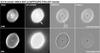 |
Fig. 1 Example of the magnification process for IC 418. Shown are the images in [O iii] and [N ii] (left two columns). The third column shows the signal of expansion, and the fourth shows the difference after the first-epoch image was magnified by a factor M before subtraction (see text for more details). Corresponding sets of images for the other targets are found in Appendix B. |
We would like to emphasize here that the age as defined by Eq. (1) should not be mistaken as the real post-AGB age. Rather, it represents the present timescale of expansion of the measured feature. The real age is usually higher because of the accelerated nebular expansion. A thorough evaluation of the offset between the kinematic ages from Eq. (1) and the real ones by means of radiation-hydrodynamics simulations can be found in Schönberner et al. (2014). Especially for young objects with cool central stars, the real (=post-AGB) age can be higher by 20–100%.
We also caution the reader that difference and residual images allow us to recover only the proper motions of edges and not the bulk changes in the smoothly distributed gas that represents nearly all of the nebular mass. Also, if sharp edges are associated with material at or behind a shock, we stress that we are measuring the motion of the shock pattern, not the motion of gas that continuously streams through the shock (Mellema 2004, hereafter M04; Schönberner et al. 2005b, herefater SJS). Similarly, changes in location of an ionisation front (IF) mark the far penetration distance of stellar ionizing radiation but not the motion of gas through which the IF and its leading shock penetrates further into neutral gas.
M04 and SJS have shown that the Doppler speeds measured from emission lines at or near the sharp edges may disagree with the apparent proper motions (converted to km s-1) of shock locations and edges measured from images such as ours by as much as 20% or more at various times during the evolution of the nebula. Correction for this discrepancy is critical for measuring accurate expansion parallaxes.
Table 2 lists our fits to global nebular expansion rates derived from pairs of high-quality WFPC2 images through the same filters. By “global” we refer largely to the loci of bright rims, the edges of shells, or ionisation fronts that define the large-scale morphology of each PN inside its halo. A single magnification factor M was usually sufficient to describe the expansion of the nebular feature in question.
2.3. Nebular diameters
Diameters along the minor axes of our sample objects.
In this section, we report on our efforts to measure accurately the angular sizes of the structures whose proper motions are used for distance determinations. We measured exclusively along the minor axis because the nebular structures are usually cleaner along this axis and the measured angular diameter is not affected by the nebula’s inclination.
We proceeded as follows: using intensity cuts of the images along the minor axis, we measured the distance between steep slopes located on opposite sizes of a feature (rim or shell) just above the outer base of the slopes. The exact placement of the measuring position is obviously subjective, but we tried to be as consistent as possible. This is the most consistent way to measure diameters for much noisier nebulae where noise and asymmetries will render most numerical methods unreliable without first fitting splines.
Most PNe are easy to measure, but some are not. Sometimes the edges are amorphous or filamentary, so the determination of an edge is ambiguous. In other cases the edges are faint and difficult to identify. In such cases the line ratio method is preferred (see below). Even so, the uncertainties are large. In three cases, the rim is clearly broad and the [N ii] diameter is larger than that measured from Hα or [O iii]. In each case (NGC 6565, NGC 7027, and IC 418), the edge looks like an ionisation-recombination front, not a sharply defined brightness discontinuity that supersonic gas flows will produce. We suspect that NGC 3132 and NGC 6886 are also in this class; cf. Figs. B.5 and B.14. We guess that the rim of BD + 30°3639 is also an ionisation front with holes in it (Fig. B.1). If so, some of the stellar UV leaks through into a shell whose leading edge is too faint to be seen.
We present our minor axis diameters of rims and shells in Table 3 where we also compare our shell diameters with the nebular diameters recently measured by Frew (2008). Note that Frew’s values correspond to the 10% intensity level. In cases where no shell is visible, the Frew diameter refers to the rim. In general, there is very good agreement between our and Frew’s diameters: The differences do not exceed the 20% level, except for NGC 6543 in which the definition of the minor-axis diameter is ambiguous (see Table 3).
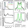 |
Fig. 2 Snapshot of a hydrodynamical PN model (left column) and comparison with observable quantities like [O iii] λ 5007 Å surface brightness (top right) along the minor axis and central line profile (bottom right) of IC 2448. Symbols are the observations, solid lines the model predictions. The model is from a sequence introduced in Steffen & Schönberner (2006, Fig. 6, right panel which utilizes the “revised” wind model of Pauldrach et al. (2004). The parameters of the model are given in the legend. The PN model proper extends from 1.5 × 1017 cm to 5 × 1017 cm, consisting of a high-density part, the “rim”, and a low-density part, the “shell”, both embracing the shock-heated “bubble” (cavity). The top left panel gives also the ion density distribution (total, He2+, O2+, N+), the middle panel: the radial velocity field, and the bottom panel: the electron temperature. The two tiny temperature spikes indicat the leading shocks of rim and shell, respectively. The shell engulfs halo matter (former AGB wind) where the history of the final AGB evolution is stored, and the rim engulfs the slower upstream matter of the shell. The weak appearance of the shell as seen in the surface brightness and line profile reflects the density difference between rim and shell, although most of the nebular mass (up to about 80%) resides within the shell. |
3. Expansion properties of PNe
3.1. Theoretical considerations
Nearly all of the past expansion parallax studies have assumed that nebular expansion speeds and corresponding Doppler expansion speeds are the same. However, PNe expand owing the rapidly varying effects of the global momentum flow derived from ultraviolet heating and local shocks induced by highly supersonic stellar winds. Thus proper motion measurements tend to focus on thin, bright shock-compressed gas whose location propagates through the nebula; that is, they represent the history of an evolving pattern. The Doppler velocities, however, are dominated by the expansion of nebular gas as integrated through its corpus, that is by bulk motions. The ratio of the two speeds must therefore be corrected for these differencs. The correction factor must be determined by hydrodynamic models, as recognized by Marten & Schönberner (1991), Marten et al. (1993), Mellema (1994, 1995), Schönberner & Steffen (2003), and M04.
Since then 1D detailed radiation hydrodynamic models including realistic stellar evolution have appeared (Perinotto et al. 2004; Schönberner et al. 2005a; SJS; Jacob et al. 2013, and references therein). These can be used to derive accurate expansion-parallax distances. These new 1D radiation models are fully time-dependent and predict the evolving expansion rates and loci of shock-compressed gas of PNe formed by stars of different masses, ejection mass fluxes and wind speeds, global heating rates from ionizing radiation, and the propagation and mass redistribution effects of highly supersonic stellar winds.
An example of how these models compare with real objects is shown in Fig. 2. Although our hydrodynamics simulations were neither aimed at nor fine-tuned for fitting any particular object, the agreement with, e.g. IC 2448, ist surprisingly good. The model has well-developed rim and shell structures and a radial velocity field not really similar to a Hubble-like law v(r) ∝ r. Instead, we see two nested shock waves which are driven by two different kinds of pressures and expand completey independently of each other. The temperature spikes seen in the temperature panel of Fig. 2 indicate the radial positions of their leading shocks. The flow velocity at the outer shell edge (~28 km s-1) is much higher than the corresponding rim velocity (at the inner shell edge) of about 18 km s-1. However, the higher shell velocity is hardly seen in the [O iii] line profile, although the shell is clearly visible in the surface-brightness distribution.2 We note that Sabbadin et al. (2004) finds a similar velocity structure in NGC 7009, although the authors incorrectly presumed that the nebular expansion speed is proportional to distance from the star (see discussions in Sects. 3.3 and 4.1, and in Perinotto et al. (2004).
The ionisation sructure of this model is also interesting. While O2+ follows closely the total density distribution, except for the innermost regions where O3+ dominates, N+ is mainly concentrated towards the outer shell where the stellar UV flux is geometrically diluted; He2+ is still restricted to the rim.
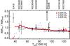 |
Fig. 3 Ratios of measured rim and shell expansion timescales (kinematical ages), i.e. |


3.2. Global expansion of rim, shell, and microstructures
All the theoretical aspects discussed above refer only to the optically-thin phase of nebular evolution. We postpone the treatment of the four optically thick objects mentioned above (Sect. 2.3) to a separate subsection (Sect. 4.7).
Before continuing with our main goal, the determination of distances, we would like to discuss global aspects of the PN evolution as they follow directly from the measurements listed in Table 2 and to compare them with the predictions of modern radiation-hydrodynamics simulations of PN evolution.
3.3. Rims and shells
We show in Fig. 3 the measured timescale ratios of rim and shell expansion listed in Table 2 vs. the effective temperature of the respective central stars. The stellar temperature is a useful distance-independent proxy of the evolutionary time across the Hertzsprung-Russell diagram (HRD) because the two most important processes which rule the nebular expansion, the radiation field and the stellar wind, depend directly or indirectly on the stellar temperature. Furthermore, the total range of the stellar temperature does not depend much on the central-star mass. The high sensitivity of the post-AGB evolutionary timescale on the stellar mass is thereby eliminated.
The message from Fig. 3 for stars with Teff ≲ 8000 K is clear: within the observational errors, rim and shell edges initially expand, by accident, with about the same speed. There is, however, an indication that the rim’s expansion timescale is a little longer at the beginning than that of the shell (IC 418). Later, the rim becomes more accelerated, and its expansion timescale falls eventually below that of the shell (NGC 7662, NGC 3918). IC 418 and NGC 3242 are significant exceptions to be discussed in the next paragraph.
These observations are consistent with the predictions of the hydrodynamic model calculations for which three examples are also shown in this figure. These model calculations show the general trend of decreasing rim and shell age ratios from about unity to values well below unity. We remind the reader that it is simply the rapid increase of thermal shell pressure due to photoionisation-heating that prevents the wind-blown bubble to expand rapidly enough into the photoionized shell. The latter is, in turn, accelerated because of the negative density gradient build up during the last mass-loss phase during the final AGB phase of evolutiony (e.g. discussed in Schönberner et al. 2014). This general trend is interupted by the transition from the optically thick to the optically thin nebular stage during the early evolution and by the passage of the He ii ionisation front through the rim-shell interface. In both cases, the rim or shell kinematical age ratio can well be higher than unity. IC 418 belongs obviously to the first and NGC 3242 to the second case.3
For obvious reasons the model sequences shown in Fig. 3 are illustrative examples of PN evolution and not a fit to the observations. We note, however, that the optically thick-thin transition of the 0.595 M⊙ model sequence shown in Fig. 3 occurs at an stellar effective temperature of about 50 000 K, obviously later than it occurs for IC 418, and at this temperature both the observed objects (NGC 6891 and NGC 6826) are already optically thin. We remind the reader that the moment when a nebula becomes optically thin dependes sensitively on the nebula’s initial density distribution and the central star’s properties such as luminosity and mass (i.e. evolutionary speed). Also, the amplitude of the age ratio caused by the passage of an ionisation front depends on the prevailing densities. Thus we are confident that appropriate adjustments of the initial model parameters would suffice in order to bring the models into better agreement with the observations, that is, with the time of the thick-thin transition and the corresponding age-ratio amplitudes.
A cautionary note, however, is necessary here: As already mentioned previously in this paper (Sect. 2.1) and what will be discussed more explicitly in Sect. 4.2, the measured expansion rate does not necessarily trace exactly the propagation of the respective shock. This is especially a problem for the rim because its leading shock is weak and the rim’s density distribution is mainly controlled by the rapid variation of the bubble’s thermal pressure along the evolutionary track and not by shock compression, as is the case for the shell’s shock. However, because the rim is always (and remains) quite thin with respect to the extension of the whole nebular structure, we do not expect significant errors when comparing the observations with the predictions of our hydrodynamics models.
We mention in passing that the measured behaviour of rim and shell expansion in the plane of the sky is fully consistent with the respective radial velocity measurements along the central line of sight. This can be seen in Fig. 9 of Schönberner et al. (2014) where (for many stars in common with the present work) the (Doppler) expansion velocities of rim and shell are plotted against the effective temperature of the respective stars. While the rim (Doppler) velocities do not exceed about 10 km s-1 for all objects with cooler nuclei (Teff ≲ 60 000 K), they increase to about 30 km s-1 for the objects with the hottest central stars. In contrast, the corresponding shell post-shock velocities vary only modestly from about 10–30 km s-1 to about 40 km s-1. Thus also the Doppler velocities reflect decreasing expansion timescales with evolution.
The close agreement between rim and shell expansion timescales as seen in Fig. 3 is purely fortuitous and should not lead to the presumption (as is done frequently) that PNe expand with flow velocities v ∝ r. This interpretion is physically incorrect since we measure only the expansion of leading shocks (or features closely associated to them). The flow of matter behind (or in between) these shocks is entirely ruled by hydrodynamics and is only very loosely described by a v ∝ r law. A suite of radial velocity profiles expected from (1D) hydrodynamics can be seen in Perinotto et al. (2004).
3.4. Microstructures
Systems of knots and networks of filaments are also observable in almost half of our sample, especially in the F658N filter. These reveal “microscale” structures whose displacements over a decade can also be measured from the HST images. As seen in Table 2, and illustrated in Fig. 4, most of the proper motions of the microscale features do not track those of the larger structures in which they are embedded.4 Either these small features were formed when the nebula was ejected from the envelope of the pre-PN star or they condensed as instabilities in the outflowing gas at a later time. Moreover, there is no obvious sign that knot formation has much of an impact on the global morphologies of PNe.
The fast low-ionisation emission regions (FLIERs) seen in NGC 3242 and NGC 6826 are two poignant cases. Their proper motions lag those of the global features in which they are found, suggesting a larger age if they have not been decelerated. This peculiar expansion behaviour of the FLIERs can be nicely explained if the early growth patterns of post-AGB winds are constrained by poloidal magnetic fields in the ISM (van Marle et al. 2014, their Fig. 17), though poloidal fields are generally weak.
An exception from the general trend is seen for NGC 6543. The data used in Fig. 4 refers to the feature called “E105” for which we have already found faster expansion with respect to the central bubble. See Balick & Hajian (2004) for more details.
4. Expansion distances
4.1. Basic methodology
In its simplest form, the distance determined using the expansion parallax method, or “expansion distance” Dexp, in parsecs, is given by  (2)(e.g. Reed et al. 1999), where VDoppler is the flow velocity in a nebular shell, deduced from a suited Doppler-split emission line observed in the direction to the nebular centre (in km s-1), θ the angle between the centre of the nebula and the feature being used to determine its expansion (here the nebular edge), and
  (3)is the overall angular expansion rate (in milliarcseconds per year, or mas yr-1) of this feature. Values of M − 1 and Δt are provided by Table 2, the angular radii can be derived from the diameters listed in Table 3.
We make the presumptions that
-
(i)
the rim and the edge of the shell can have different fractionalexpansion rates (i.e. kinematic ages); and
-
(ii)
the rim (or the edge of the shell) can be characterized by a single expansion age (that is, expansion factor M). This is verified because one value of M works for the entire rim (or shell), even for relatively elliptical objects (cf. Table 2).
If it were the case that the rim and the shell were simple ballistically expanding entities, then the expansion parallax method works without correction. However, the hydrodynamical models show that nebulae shaped by winds and thermal pressure do not expand uniformly. The rim is shell material that has been displaced and swept-of by the growth of the overpressured cavity inside of it. Its sharp leading edge is actually a pattern feature associated with the shock.
In our models, the rim forms later than the shell (as the wind luminosity ramps up), and – after a phase of stalling – it becomes accelerated.5 It can be used to derive expansion distances provided that the position of the evolving rim and its expansion speed are carefully measured and interpreted (see below). As noted earlier, the leading edge of the shell is sweeping supersonically into lower density gas upstream. Its very sharp edge attests to the presence of this upstream gas. The shock interface is formed by inertial resistance and steady pressure of the shell. The density compression at the leading edge of the shell is very mild, its progress is steady, and the location of its shock is simple to determine from well-exposed images. From a hydrodynamical standpoint, the leading edge of the shell is a more robust (albeit fainter) feature to use for distance studies.
In particular, the location of the outer edge of the shell is a much simpler fiducial because the angular expansion speed of its edge is nearly proportional to the flow speed of the gas behind that edge (shock) and the shock properties, thus the correction factors to be applied, do not change much during the expansion. Moreover, the shell shock’s upstream matter (i.e. the halo) has often an obviously quite spherical shape (cf. Corradi et al. 2007), which implies that our assumption of spherical expansion is better fulfilled than for the rim.
The edge of the rim consists of compressed gas that follows a shock whose precise location is not easily extracted from images in which the shock itself is not resolved (M04; SJS). That is to say, the location of the shock is determined by the density gradient at the leading edge of the rim and not the brightness distribution of the rim after convolution by the telescope PSF. The proper motions of the rim need to be corrected by factors of 1.2 up to approximately three – or better still determined using the simulated density and shock structure from hydro models that properly compute the emissivity of the emission lines at every point in the post-shock zone where the detected light is emitted (discussed in Sect. 4.2).
Some objects could not be (fully) considered for distance determinations, for the following reasons:
-
BD + 30°3639:
This is the onlyobject of our sample with a hydrogen-poor [WC] central star,implying that our hydrodynamical models are not appropriate forinterpreting the angular expansion of the nebula. The reason is themuch higher mass-loss rate that is typical for Wolf-Rayet objects.Without a hydrodynamic model it is not possible to correct for thedifference between pattern and matter velocities. Additionaly,the images of BD + 30°3636do not show distinct features like shell or rim edges whose propermotions could be measured unambigously.
-
NGC 2392:
It was difficult to assign appropriate flow velocities to rim and shell angular expansions.
-
NGC 6210:
Rim and shell are too irregular.
-
NGC 7027:
Uncertain magnification (cf. Table 2) because optical light from the compact ionized nebula is heavily obscured by irregularly distributed foreground dust.6
-
NGC 6891:
Here the outer edge of the shell is faint, and its radius is systematically affected by problems with CTE1. Nevertheless, we were able to derive a reasonable distance.
4.2. Lessons from hydro models
For the distance determinations we follow a new, more physically based approach: we combined the basic methodology just discussed with the knowledge gained from the hydrodynamical simulations of PN formation and evolution in order to derive the so far most reliable distances to many of the objects presented in this paper. This more physical approach includes the important offset between shock and the (measurable) flow speed not considered in the basic approach used hitherto. This offset is such that Eq. (2) always underestimates the distance by at least 20–30%. The physically correct version of Eq. (2) is then  (4)where Ṙshell/rim are the true expansions of the rim or shell edges (in km s-1) and
  the corresponding angular expansions in the plane of sky (in mas yr-1).
The first attempts in this direction have been made by M04 and SJS who applied appropriate correction to distances based on Eq. (2). M04 derived the corrections from the shock jump conditions taylored to the conditions prevailing in PNe while SJS used predictions from detailed radiation-hydrodynamics simulations of PN evolution. Both methods arrive at correction factors that are in good agreement with respect to the size of the corrections and their differences between rim and shell (see below).
We note that all previous attempts for deriving expansion parallaxes (except the study of IC 418 by Guzmán et al. 2009) have exclusively used the bright nebular rim, for obvious reasons. Here we employ also the shell for a larger number of objects and for reasons just mentioned above. The fractional increase of both nebular structures, rim and shell, should lead, of course, to the same distance if the method used here, that is, employing hydrodynamical corrections, is reliable. On the other hand, agreement or disagreement between rim and shell parallaxes is a criterion on our present understanding of PN physics.
The shells.
Once the apparent expansion of the shell’s outer edge (=expansion of the shock front) in the plane of the sky has been determined, we combined it with the post-shock velocity measured from carefully analysed emission-line profiles that have been observed through the central line of sight: here we assumed that the nebula is spherical or slightly prolate in shape and growth and that the shock expands uniformly in the nebular midplane. This appears to be justified given that the shock propagation speed depends only on the upstream density gradient and not on the density itself (Chevalier 1997; Shu et al. 2002) and that the smooth shell upstream from the rim usually has a more spherical shape than the rim itself (Corradi et al. 2003; Schönberner et al. 2004). Accordingly, corrections due to a possible aspherical expansion are very small.
The concept of the post-shock velocity and how the latter can be determined has been introduced by Corradi et al. (2007) and expanded by Schönberner et al. (2014) where the shell’s post-shock velocities for a large sample of PNe can be found. Using radiation-hydrodynamical models, Schönberner et al. (2014, Fig. 6 therein) demonstrated that, once the model becomes optically thin to Lyman-continuum photons, the ratio between post-shock flow velocity and shock speed does not change appreciably during the evolution across the HR diagram. Specifically, for optically thin PN models the relation  (5)holds, where Vpost (post-shock velocity) is the flow velocity immediately behind the shock with radius Rshell, and Ṙshell is the edge (=shock) expansion speed. The distance Dexp to a particular object follows then via Eq. (4):
  (6)M04 proposes a correction of about 20%, that is, a correction factor of about 1.20. This correction factor changes only slowly with shock speed: from Mellema’s Fig. 6, we extract, for example, a 20% correction for a typical Vpost = 40 km s-1, but 25% for 30 km s-1. For very low post-shock velocities, say 20 km s-1, the correction is about 30%. Given that M04 used only a fixed value for the (isothermal) sound speed (corresponding to 10 000 K), the agreement with our hydrodynamical simulations is excellent. We conclude that our correction factor (and its uncertainty) used in Eq. (2) is quite robust and is valid as long as the nebula is fully ionised.
The rims.
The situation is more complicated for the rim, as already mentioned earlier. The leading shock is weak (Mach number about 1), and the density distribution between shock and contact discontinuity is rather ruled by the pressure balance between rim and hot bubble and is thus subject to the nebula’s evolutionary stage. Because of this, the expansion velocity of the bulk rim matter measured spectroscopically, Vrim, does not usually correspond to the shock’s post-shock velocity in a simple way.
The ever changing wind luminosity while the central star crosses the HR diagram is responsible for the matter and velocity distribution within the rim. An impression about the influence of the wind model used in hydrodynamical simulations is seen in Fig. 6 of Steffen & Schönberner (2006) where where the surface brightness of two nebular models with the same parameters but with different mass-loss histories are compared. We note that only the rim is influenced; the expansion of the shell remains completely unaffected by the changing wind properties.
Based on the jump conditions for shock waves, M04 derived a relation such that the ratio between shock and post-shock velocity,  , can be expressed by the other flow variables (his Eq. (4) where our FM is called ℛ). Using the very good approximation of an isothermal (γ = 1) and weak (Mach number = 1) shock, this ratio FM is plotted in Fig. 5 over
  for different assumption of the electron temperature, represented by the (isothermal) sound speeds cs.
 |
Fig. 5 Ratio |

![Mathematical equation: \hbox{${F = \dot{R}_{\rm rim}/ V_{\rm rim}^{\rm [O\,III]}}$}](/articles/aa/full_html/2018/01/aa31788-17/aa31788-17-eq129.png)
![Mathematical equation: \hbox{$V_{\rm rim}^{\rm [O\,III]}$}](/articles/aa/full_html/2018/01/aa31788-17/aa31788-17-eq130.png)
Distances from shell-edge expansion.
It is clearly seen that especially for low flow velocities, shock and post-shock speeds differ considerably, that is, F can be higher than two. The ratio FM shown in Fig. 5 depends on the assumed (isothermal) sound speed: the curve is shifted downwards for lower and upwards for higher electron temperatures. If the Mach number increases, FM becomes smaller and the run with post-shock or rim velocity is flatter (cf. M04).
Since for the rim’s case the post-shock velocity is not observable, we have to rely on Vrim only (from the line of sight splitting of the main line-profile components) and need an appropriate correction in order to account for the difference between the bulk velocity Vrim and Ṙrim, the shock’s expansion velocity. Here we utilise again our radiation-hydrodynamics models where we know Ṙrim and the observable Vrim and compute  vs. Vrim (instead of ). The result is also shown in Fig. 5 and is very similar to Mellema’s theoretical approach. The correction factor F decreases also with increasing Vrim. It is important to realize that F is quite large (between two and three) for very low rim velocities, as is typical for unevolved objects. Later, if the rim expands faster, F approaches values which are typical for the shell, that is, values closer to unity.
Given the fact that the run of F with Vrim is rather smooth, not much model-dependent and very similar to the simple theoretical considerations, we are confident that our models allow a reasonable estimate of the correction from bulk rim velocity to rim shock velocity, and we therefore applied the following relation for determining rim expansion distances: 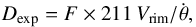 (7)where F depends on the observed Vrim and is read off from the models shown in Fig. 5. Specifically, we use F as predicted fom the 0.595 M⊙ model because its rather smooth run with Vrim.
For completeness we note that the relations shown in Fig. 5 hold also for [N ii].
4.3. Results for shell expansion
For all objects from Table 2 with reasonably measured shell edge expansion and known post-shock velocity, distances via Eq. (6) were determined for the first time. For consistency we took individual post-shock velocities from Table 1 in Schönberner et al. (2014), although the differences beween velocities from [N ii] and [O iii] are, if at all, usually very small. The resulting expansion distances are listed in Table 4, together with the relevant input parameters.
IC 418.
This object is still optically thick, or marginally optically thick, and Eq. (6) is not applicable since the shell’s leading shock and the ionisation front are virtually at the same radial distance from the star. A good tracer of the ionisation front and its expansion speed is the [O i] λ 6302 Å line, but here we have also to consider the strong radial increase of density and flow velocity, as is typical for this phase of evolution (see, e.g. Fig. 3, top panels, in SJS). Together with the projection effect, the line-peak separation measures thus a somewhat lower velocity. This difference depends on the exact phase of evolution, but using our hydrodynamic models we estimated factors between 1.2 and 1.4 for converting the [O i] line-peak separation velocity into the shock/ionisation front velocity for the rather short evolutionary phase of the transition from the optically thick to the optically thin stage. We used, therefore, a factor of 1.3 ± 0.1 instead of 1.25 for the case of IC 418.
This is the only object from Table 4 whose shell expansion has been measured previously by means of radio continuum observations with a time baseline of about 21 years (Guzmán et al. 2009). These authors found an angular expansion of 5.8 ± 1.5 mas yr-1. Our value from optical HST images is a bit smaller but much more accurate: 5.2 ± 0.5 mas yr-1 (cf. Table 4). Guzmán et al. (2009) combined the angular expansion with a flow velocity of 30 km s-1, derived from an empirical expansion law found by Morisset & Georgiev (2009) and arrived at a distance of 1.1 ± 0.3 kpc without and 1.3 ± 0.4 kpc with gas dynamic correction as proposed by M04.
We believe that our approach to use a measured velocity (here 22 km s-1 from [O i]) is more reliable. Our smaller angular expansion rate and smaller flow velocity combine such that we arrived at nearly the same distance but with a reduced uncertainty: 1.16 ± 0.20 kpc.
4.4. Results for rim expansion
Distances from rim-edge expansion.
The distances from the rim parallaxes are listed in Table 5 along with the corresponding correction factors. The spectroscopic bulk velocity of the rims, Vrim, is taken from the most recent literature, that is, from Schönberner et al. (2014) if not otherwise stated. In Table 5, we did not correct the measured Vrim for rim orientations as did, for example, Palen et al. (2002). As long as all Doppler line width measurements pertain to the central line of sight only no inclination corrections are necessary.
IC 2448, NGC 6578.
These two objects have already been studied by Palen et al. (2002) using HST images about four years apart. Our time span is twice as long as theirs, and comparing Palen et al.’s magnification data with ours, we find fair agreement: 2.25 ± 0.60 vs. 2.7 ± 0.2 mas yr-1 (IC 2448, mean from Table 5) and 1.6 ± 0.4 vs. 2.4 ± 0.4 mas yr-1 (NGC 6578, mean from Table 5).
NGC 6543.
Miranda & Solf (1992) have shown that NGC 6543 is structurally and kinematically complicated, making it a less-than-ideal nebula for our purposes. This object has been analysed by Reed et al (1999) using HST images with a baseline of three years only. We used images with a baseline of 13 years, and our angular expansion rate of 3.13 ± 0.16 mas yr-1 is consistent with the older measurements of 3.4...3.6 mas yr-1, but now with a much smaller error, that is, 0.16 instead of 0.9 mas yr-1.
Balick & Hajian (2004) studied this objects over a time span of 6 years and with more sophisticated analysis methodologies. Among other things, they found (and we verify) a very complex expansion pattern which 1D radiation hydro models cannot fit well. They also found (as do we) that no single value of M characterizes the inner bubble (Mmajor>Mminor). They found Dexp = 1.0 kpc after adopting a value of F = 1. Frew (2008) used this object as calibrator, but with a corrected expansion parallax as recommended by Mellema (2004), that is, with a factor of 1.5 and a corresponding distance of 1.50 kpc (Frew 2008, Tables 9.5 and 9.6 therein), a little lower than the distance of ≃1.85 kpc found here (cf. Table 5).
NGC 3242, NGC 7662.
For both objects, expansion measurements have been reported by Hajian et al. (1995) and Hajian & Terzian (1996) with the radio technique. Our measurements are based on a longer time baseline with much smaller errors and differ considerably: 13.2 ± 4.7 vs. 4.8 ± 0.3 mas yr-1 (NGC 3242) and 5.6 ± 5.0 vs. 3.5 ± 0.3 mas yr-1 (NGC 7662). We are unable to present any explanation of these differences. However, our new and more accurate angular expansion rates measured for NGC 3242 and NGC 7662 lead now to significantly larger distances than before, resulting in luminosities which are now in good agreement with predictions of post-AGB evolutionary models (cf. Sect. 6).
4.5. Comparison between N II and O III distances
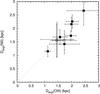 |
Fig. 6 Distances from [N ii] images vs. distances from [O iii] images for objects with measurements in both filters. Open squares are for shell (3) and filled square for rim measurements (7). |
Hajian (2006) noted, based on [N ii] and [O iii] data of 8 objects, that there might be a trend of the [N ii] distances to be somewhat larger than the [O iii] distances. Here we have 7 PNe with expansion measurements from [N ii] and [O iii] images, 4 PNe of which have additionally also data from both the shell and rim available. Although the number of measurements is comparable, we found no sytematic trend between [N ii] and [O iii] distances, neither for the rim nor shell (see Fig. 6).7
In principle, this outcome is to be expected: the kind of PNe investigated here, that is, with a well-defined rim-shell structure, are fully ionised, and lines from the N+ and O2+ ions trace virtually the same nebular regions. The small difference between the [N ii] and [O iii] bulk rim expansion velocity observed for some objects is too small as to have, within the errors of the proper-motion measurements, a significant influence on the distance determination.
Because of the close agreement between [N ii] and [O iii] results, we will not distinguish between them in the following sections. Instead, we will use their average value, weighted according to their individual errors.
4.6. Comparison between rim and shell distances
In the previous sections we have been able to derive distances from rim and shell expansions measured separately and corrected individually by means of predictions based on hydrodynamic nebular models. In principle, both measurements should give the same answer if our assumptions were indeed justified. There are only three objects for which both rim and shell distances are available with sufficient accuracy, and Fig. 7 shows the comparison, separated into [N ii] and [O iii].
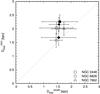 |
Fig. 7 Comparison of shell and rim distances for the three objects for which reliable shell data exist (cf. Tables 4 and 5). Open symbols are for [O iii], filled for [N ii]. |
It is evident from this figure that there is, within the errors, a good correspondence between the distances deduced from the expansions of the rim and shell edges, though it appears that the shell distances are a bit smaller (except for NGC 6826). The number of objects with both measurements is, however, too small as to allow a firm statement. We note that this rather close agreement with both distances is only possible because of two very different correction factors, viz. 1.25 for the shell and about two for the rim for the case of NGC 6826! We are thus confident that also the expansion of rim edges, if appropriate corrections are applied, yields reasonable distance determinations.
4.7. Optically-thick, evolved PNe
Distances for evolved, optically thick objects.
4.7.1. General considerations
We noted above (Sect. 2.3) that four objects of our sample are in a very evolved stage with very hot central stars (>100 000 K) and nebulae which are obviously optically thick to Lyman ionizing photons. These objects can be separated into two groups: those with still rather luminous central stars (≳ 103L⊙, NGC 6886 and NGC 7027), and those with low-luminosity central stars (<103L⊙, NGC 3132 and NGC 6565). NGC 7027 will not be considered further here because no single magnification factor could be found (cf. Table 2).
We note that IC 418, although still mainly optically thick, does not belong to the group of objects considered in this section. It is an unevolved, very young nebula with a luminous central star which is just in the transition to become optically thin with and has been already treated in conjunction with the other optically-thin nebulae.
Measurements along the minor axes of the three remaining objects show clear indications of ionisation stratification: their [N ii] diameters are a bit larger than the [O iii] diameters (cf. Table 3). This is a clear indication of ongoing recombination or already beginning reionisation, depending on the stellar flux of ionising photons. Still dense nebulae around fast evolving stars recombine already well before maximum stellar temperature because the fluxes of ionizing photons decrease once a certain stellar temperature is reached, viz. about 60 000 K for Lyman photons (see, e.g. Fig. 7 in Schönberner et al. 2007). Less dense nebulae around more slowly evolving stars may only recombine (to different degrees) after the fast luminosity drop of the star when it settles onto the white-dwarf sequence.
The process of recombination disturbs the relatively simple double-shell structure which is typical for the high-luminous, optically-thin phase of evolution. For PNe ionised by geometrically diluted stellar photons and whose densities decline more slowly than r-2, recombination starts at the outer nebular edge and proceeds inwards with a timescale controlled by the local ion and ionising photon density.8 After the stellar luminosity drop, recombination and reionisation occur at the same time but at different places within the nebula: reionisation close to the star and still ongoing recombination further out. We note that neither recombination nor reionisation always manifest themselves by a sharp, well-defined “front” such as one finds during early evolution. Instead, both fronts are often radially smeared because of the rather low nebular densities and photons with a wide range of energies and corresponding mean free path lenghts. It is clear from these considerations that only fully time-dependent calculations (such as ours) are suitable to model this kind of late nebular evolution.
The reionisation stage is long-lived and occurs on the expansion timescale of the nebula, while recombination is relatively short, ruled by the rapid evolution and dimming of the central star. Thus nearly all nebulae around faint central stars must be considered to be in their reionisation phase.
Concerning the determination of expansion parallaxes, one must consider the consequences of ionisation stratification. During reionisation, N+ (and O+) is built up from the outer edge and is moving inwards. The O2+ concentration is restricted to the inner region only, closer to the central star. This kind of stratification also remains during the reionisation phase because the central star is not luminous enough as to ensure full ionisation as is typical during the high-luminous phase of evolution. Because of this, only lines from [N ii] (or [O ii]) are suited to tracing the outer edge of the visible nebula, that is, the old (recombination) or new (reionisation) leading shock. The positive velocity gradient leads then often to higher line-peak separations for [N ii] as for [O iii]. Therefore, only lines of species with a low degree of ionisation, for example N+, should be used in studies of optically-thick nebulae where the expansion velocities play a decisive role.
4.7.2. Applications
In order to derive expansion distances to the evolved, optically-thick objects NGC 3132, NGC 6565, and NGC 6886, we proceeded as follows: first we tried to pin-down the evolutionary stage of the three objects in question. For this purpose, we selected models from our suite of 1D radiation-hydrodynamic sequences which match the observed intensity distributions along the minor axis, at least qualitatively. Then we determined the factors necessary for correctiong the difference between the expansion velocity given by the line-peak separation and the expansion of the respective shock. We also determined the run of the correction factors as a function of the emission-line peak-separation velocity of [N ii]. The details of the whole procedure are outlined in Appendix A.
The resulting distances for these three objects, together with the other relevant parameters, are collected in Table 6. Because the procedure for obtaining the correction factors as outlined here is not at all straightforward, it is interesting to compare our expansion distances with other individual distance estimates, viz. from the extinction method and/or H i line absorption along the line of sight:
-
NGC 3132.
The central object is most probably a wide binary witha central-star companion of spectral class A0 (Ciardulloet al. 1999). Assuming that the Astar is still in its main-sequence stage, Ciardulloet al. (1999) determined a distanceto NGC 3132 of
 pc, well below our value of 1.24 ± 0.30 kpc but with overlapping error bars. NGC 3132 is also in the list of Gaia distances provided by Stanghellini et al. (2017): 656 ± 157 pc, somewhat lower than existing estimates and surely in conflict with our parallax measurement.
 -
NGC 6565.
Gathier et al. (1986a) report an extinction distance of 1.00 ± 0.44 kpc, much lower than our value. However, looking at their EB − V/(m − M)0 diagram, a distance up to about 2 kpc appears also possible. More recently, Turatto et al. (2002) estimated an extinction distance of 2.0 ± 0.5 kpc, which agrees quite well with our expansion distance of 2.19 ± 0.67 kpc.
-
NGC 6886.
This is with 4.62 ± 1.00 kpc the most distant object of our sample. The H i line absorption provides only a lower limit of 1.7 ± 0.7 kpc (Gathier et al. 1986b).
5. Final expansion distances and their discussion
In this section, we compare our derived distances (appropriately averaged, if possible, over the [N ii] and [O iii] observations and over the rim and shell measurements) with other determinations, either individually or statistically based. The final distances for those objects where we believe they are reliable (15 objects) are collected in Table 7 and compared with the statistically based distances of Frew et al. (2016) and Stanghellini & Haywood (2010) and with individual distances by means of detailed spectroscopic analyses of photospheric and/or wind lines (Méndez et al. 1992; Pauldrach et al. 2004; Kudritzki et al. 2006).
Our adopted expansion distances, Dexp, and comparisons with other determinations.
5.1. Stastistical distances
We begin our comparison with Fig. 8 which shows our distances Dexp (from Table 7) compared to those based on the Frew et al. (2016) calibration. The overall agreement is quite satisfactory, but discrepant cases do exist: NGC 6543, NGC 6891, and to a lesser degree NGC 3242 and NGC 7662. However, one should not forget that nearly all of our objects from Table 7 are used by Frew (2008) and Frew et al. (2016) as calibrators whose distances are either based on earlier expansion measurements or the gravity method. Thus, the close agreement between our expansion distances and the those from the surface-brightness–radius relation of Frew is not too surprising.
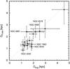 |
Fig. 8 Distances according to Frew et al. (2016) vs. our expansion distances; data from Table 7. Objects mentioned in the text are labelled. The dotted line is the 1:1 relation. |
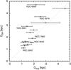 |
Fig. 9 Same as in Fig. 8, but for the Stanghellini & Haywood (2010) calibration. |
Figure 9 compares the Stanghellini & Haywood (2010) statistical distances with our results. The agreement is very good for objects with DSH< 2 kpc, but higher deviations exist for more distant objects. We note that Stanghellini & Haywood’s error estimate of 20% (0.08 dex) is in our view far too low. The Stanghellini & Haywood (2010) distances are basically the same as those of Stanghellini et al. (2008) which are calibrated by means of PNe in the Magellanic Clouds and should thus be the most reliable (in the statistical sense). For more details, the reader is referred to the cited paper.
Interestingly, two discrepant cases from Fig. 8 disappeared: NGC 6543 and NGC 7662, while the status of NGC 6891’s distance remained virtually unchanged. Two new outliers, however, appeared: NGC 6578 and NGC 6565. We are inclined to believe that our expansion parallaxes are the more reliable ones for these particular cases (perhaps with the exception of NGC 6891).
Two further comments are in order, though. We used as distance to NGC 6886 the Stanghellini et al. (2008) value of 4.4 kpc, instead of the unrealistic low value of 1.6 kpc provided by Stanghellini & Haywood (2010). Their original very high distance of 4.0 kpc to IC 2448 has been corrected by us in Table 7 because it is due to an incorrectly chosen angular radius of 5′′ which refers rather to the rim and not to the outer shell with its 10′′ radius (cf. Table 3).
5.2. The spectroscopic-gravity distances
So far we have only tested our expansion distances against the predictions of the most recent statistical methods. In this section, we will compare individual distances for the cases where also individual distances based on sophisticated spectroscopic tools are available from the literature. Three variants with different degrees of sophistification are in use:
-
The classical method of employing NLTE model atmospherestaylored to the special needs for hot and luminous central stars(Méndez et al. 1992). We prefer torefer to this paper because it provides updated parameters for allthe objects analysed in previous works. The analyses of the stellarspectra deliver Teff and surface gravity g, which are then used to estimate the mass from a Teff-log g diagram with calculated post-AGB evolutionary tracks. The distance follows then via Eq. (4) in Méndez et al. (1992), that is, D2 ∝ M/g. The implicit assumption made is the correctness of stellar evolution theory concerning the post-AGB evolution, that is, the core-mass luminosity relation. Metal line-blanketing, which reduces the effective temperature somewhat by backwarming, is not considered (cf. discussion in Kudritzki et al. 2006), and may have an impact on the gravity determination.
-
Pauldrach et al. (2004) employed a method that had been successfully used for massive hot stars with strong winds: construction of a homogeneous, stationary, extended, outflowing, and spherically symmetric radiation-driven stellar atmosphere. The blocking and blanketing of all metal lines in the sub- and supersonic region of the expanding atmosphere is treated in a hydrodynamically consistent way. The analysis relies entirely on the UV spectrum where all the important strong P Cygni lines and other wind-contaminated lines are located. A description of the underlying physics is also presented in detail in Kaschinski et al. (2012). The effective temperature is fixed by the ionisation equilibria of UV metal lines, the mass-loss rate is determined by fitting the observed spectrum, and mass and radius are constrained by the (measured and fitted) terminal velocity which scales with (M/R)1/2. This method yields, independently of other assumptions, temperature, mass, and radius, and thus one can get the distance independently of any evolutionary calculations. Strictly speaking, the distance is not based on the gravity, but because of its closeness to the two other methods we keep this variant in this group. Kaschinski et al. (2012) and Hoffmann et al. (2016) used an improved version of their code allowing also for wind clumping and analysing optical lines and confirmed the previous results from Pauldrach et al. (2004).
-
Kudritzki et al. (2006) updated the previous analyses of Méndez et al. (1992) by using so-called unified NLTE atmosphere models which include full metal line-blanketing and extend from the static photospheric region far into the wind domain. This method gives, as the authors claim, more reliable stellar parameters, especially for those objects with a strong wind, as compared to the older analyses of Méndez et al. (1992). To obtain distances, the masses are again taken from post-AGB calculations. The method of Kudritzki et al. (2006) is, however, not hydrodynamically consistent because the velocity law of the wind is adopted. On the other hand, “clumping” of the wind matter is also considered, at least rudimentarily.
The distances of Méndez et al. (1992) and Kudritzki et al. (2006) are based on the post-AGB models of Schönberner (1983) and Blöcker (1995), respectively.9 There now exist modern AGB and post-AGB calculations (Miller Bertolami & Althaus 2006; Weiss & Ferguson 2009; Miller Bertolami 2016) which employ the most recent opacities together with convective overshoot at all radiative-convective boundaries in the same (or a similar) manner to that proposed by Herwig et al. (1997). These new models are more luminous at given remnant mass (also cf. Fig. 11) which translates into a mass shift in the Teff-log g diagram of –0.04 M⊙, on the average. Since we believe that these new evolutionary calculation are superior, we will exclusively use them here. Consequently, all gravity distances of Méndez et al. (1992) and Kudritzki et al. (2006) are reduced by about –0.02 dex, or 5%, and we have already considered this systematic correction, although quite small, in Table 7 for consistency (and in Fig. 10 as well).
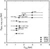 |
Fig. 10 Same as in Fig. 8, but for the spectroscopic (gravity) distances of Méndez et al. (1992), MKH (squares), Pauldrach et al. (2004), PHM (circles), and Kudritzki et al. (2006), KUP (diamonds). There are up to three spectroscopic distance per object. |
Before continuing, we remember that the spectroscopic-gravity distances turned out to be, in general at least, higher than those derived by other methods, such that stellar masses and luminosities became unreasonably high and severely disagree with the predictions from stellar evolutionary theory. We note the extreme cases claimed by Pauldrach et al. (2004): central-star masses nearly up to the Chandrasekhar mass limit have been found. With this in mind, a comparison between these distances with our expansion distances are thus of paramount importance for clearing the issue whether current post-AGB models are really incorrect.
As one sees in Table 7 and Fig. 10, the spectroscopic-gravity distances of Pauldrach et al. (2004) and Kudritzki et al. (2006) are often considerably higher than the expansion distances for all objects in common. The difference can be up to a factor of two (IC 418, IC 4593, and NGC 6826). With the exception of IC 2448 and NGC 6891, the MKH distances are close to but also systematically above (except NGC 3242) our expansion distances. The errors for IC 4593 are very big and encompasses the three spectroscopic distances. Really disturbing is, however, the fact that in those cases where three spectroscopic-gravity distance determinations exist (IC 418, NGC 3242, and NGC 6826), they disagree considerably from each other.
The lower distances found by us clearly contradict the claim of Pauldrach et al. (2004), Kaschinski et al. (2012), and more recently Hoffmann et al. (2016) that central-star masses close to the Chandrasehkar mass limit are possible for well-known objects. A discussion of their masses and luminosities on the basis of our expansion distances follows in the next section.
6. Central-star luminosities and masses
In this section, we will discuss the impact of our new expansion distances on the luminosities and masses of the respective central stars. We will also provide a comparison of our Galactic disk objects with objects for which distances are rather well known, that is, PNe in the Galactic bulge and the Magellanic Clouds.
Luminosities and corresponding masses estimated from post-AGB evolutionary tracks for our sample of Galactic disk central stars with determined expansion distances.
6.1. Galactic disk PNe with expansion distances
Table 8 gives an overview of the central-star parameters for the 15 Galactic disk objects investigated here. Temperatures and luminosities, the latter scaled to our distances, are taken from the literature as indicated. Masses of the central stars are estimated from the post-AGB evolutionary tracks used in Fig. 11. The luminosity error in Table 8 is solely based on the given distance uncertainty. The (internal) temperature error, if provided at all, is usually significantly below 10% and thus will not contribute much to the luminosity error. Moreover, temperature and radius are not indepent of each other if modern stellar atmospheres are employed for analysing the stellar spectrum.
One should, however, be more concerned about temperature discrepancies between studies on the same object performed by different authors and methods. An example is the case of IC 2448: the most recent study by Herald & Bianchi (2011), which we preferred here in Table 8, utilised next to the optical also the far-UV and UV spectral region and came up with a substantially higher stellar temperature (based on a number of metallic-line ionisation equilibria) than the classical NLTE-study of Méndez et al. (1992), viz. 95 000 K instead of 65 000 K. In this context we mention that we also preferred the higher effective temperature of 90 000 K (instead of 65 000 K) from Miller et al. (2016) for the central star of NGC 3242, simply because its nebula has nearly the same excitation as IC 2448.
Likewise, derived luminosities may depend on the analysing methods used, as one can demonstrate for the case of NGC 6826. Despite the very smilar effective temperatures (44 000–50 000 K), the luminosities differ by high margins: 7000, 3700, and 4700 L⊙ for Méndez et al. (1992), Pauldrach et al. (2004), and Kudritzki et al. (2006), respectively, if scaled to our distance of 1.55 kpc.
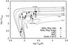 |
Fig. 11 HRD of PNe nuclei together with evolutionary tracks of hydrogen-burning AGB remnant after Miller Bertolami & Althaus (2006, priv. comm., solid). Numbers at the tracks denote the central-star masses in solar units. Tracks of AGB remnants from Blöcker (1995) and Schönberner (1983) are also shown (dashed) for comparison. Their masses are (from bottom to top): 0.553, 0.565, 0.605, and 0.696 M⊙, respectively. The 0.517 and 0.553 M⊙ remnants start their post-AGB evolution as burning helium. The upward “hooks” are due to the rekindling of hydrogen which then slows down the evolution considerably. The filled circles with the respective error bars mark the positions of the Milky Way disk objects listed in Table 8. We show also nine (hydrogen-rich) objects from the Magellanic Clouds (seven from the Large Cloud, circles, and two from the Small Cloud, squares), taken from the analyses of Herald & Bianchi (2004) and Herald & Bianchi (2007). Also, five objects from the Milky Way bulge with the parameters derived by Hultzsch et al. (2007) are displayed (diamonds). The position of K648 in M 15 is based on the recent study of Jacoby et al. (2017). |
Figure 11 shows the HRD relevant for post-AGB evolution. We employed the new post-AGB calculations of Miller Bertolami & Althaus (2006, and priv. comm.) which consider the latest opacities and a more physical description of the convection-related “overshooting”.10 The latter is treated in the same or similar way as proposed by Herwig et al. (1997) and is applied to all convective-radiative boundaries. For comparison purposes, we also overplotted older computations, viz. those of Schönberner (1983) and Blöcker (1995) which did not consider convective overshoot.
First of all, there is a significant difference between the two grids of post-AGB evolutionary tracks. At a given luminosity, the Miller Bertolami & Althaus (2006) models are less massive than the Blöcker (1995) models: for instance, 0.54 corresponds roughly to 0.57 M⊙, 0.563 to about 0.605 M⊙, and 0.661 to 0.696 M⊙. With other words, the new AGB evolutionary calculations of Miller Bertolami & Althaus (2006) reveal a new (core)-mass–luminosity relation for central stars. It starts at lower core masses and runs initially rather steep. Only for core masses above 0.7 M⊙ it approaches slowly the older relation. In the following, we will refer only to the new evolutionary calculations of Miller Bertolami & Althaus (2006).
At the lower mass end, we have added two initially helium burning models, 0.553 M⊙ from Schönberner (1983) and 0.517 M⊙ from Miller Bertolami & Althaus (2006), because of their low luminosities and comparitively short transition times from the tip of the AGB to the PNe region until hydrogen burning turns on again.
Our 15 objects from Table 8 ocuppy a well constrained region in this HRD which is embraced by post-AGB track between about 0.6 and 0.53 M⊙ (neglecting NGC 6891). By interpolating between the tracks, a mean central-star mass of 0.55 M⊙ follows.11 The corresponding plateau luminosity is about 5000 L⊙ (log (L/L⊙) = 3.7).
6.2. PNe in stellar populations with known distance
It is, of course, of paramount importance to compare our expansion-distance based sample in the HRD of Fig. 11 with objects for which distances are known a priori. We therefore supplemented our sample by objects from the Magellanic Clouds and the Galactic bulge for which detailed analyses of the central stars are available.
6.2.1. The Magellanic Clouds
Herald & Bianchi (2004, 2007) studied PNe in the Magellanic Clouds by means of FUV (Fuse) together with UV and optical (HST) spectrograms. They employed NLTE, fully metal-line blanketed atmosphere/wind models to infer effective temperatures, luminosities, and mass-loss rates of the central stars. Knowledge of the stellar gravity is not necessary.
We show in Fig. 11 the nine hydrogen-rich central stars (LMC and SMC) analysed by Herald & Bianchi (2004, 2007).12 Their positions overlap nicely with our sample, and their mean luminosity is approximately 4200 L⊙, the evolutionary luminosity decline not considered (cf. Fig. 11). There is excellent agreement with the results of our expansion-distance sample. 13
6.2.2. The Milky Way bulge
Another stellar population with known distance is that of the Galactic bulge, although the distance dispersion is bigger than that for the Magellanic Clouds. Five bright central stars in the Galactic bulge have been analysed by Hultzsch et al. (2007) using optical spectrograms, and with the known distance to the bulge (8.0 ± 2.0 kpc), the authors derived luminosties between ≃5000 and ≃10 000 L⊙ (see Fig. 11). This sample has a slightly higher mean luminosity (and hence also mean central-star mass), but within the errors it is still consistent with the other two samples, especially if one considers that, according to the authors, the sample is very likely biased towards the brightest central stars.
6.2.3. The case of K648 in M15
Of particular interest is the case of the central star K648 of the PN Ps 1 in the globular cluster M 15 because its mass set very important constraints on the formation of PNe in old and metal-poor stellar populations. Its effective temperature is well known (e.g. 39 000 K, Rauch et al. 2002), and after careful evaluation of the distance to M 15, Jacoby et al. (2017) determined recently a luminosity of 4000 L⊙ only for the central star of Ps 1.
It is intersting to see that the newly derived position of K648 in Fig. 11 fits perfectly to the positions of all other objects discussed here. This position gives a strong constraint on the mass of K648: assuming a distance uncertainty of 10.%, or 0.08 dex for the luminosity error, 0.54 ± 0.01M⊙ follows from the tracks shown in Fig. 11, because their mass-luminosity relation runs very steep in this particular mass range.14 This mass agrees well within the errors with the average white dwarf mass found for the globular cluster NGC 6752: 0.53 ± 0.02M⊙ (Moehler et al. 2004). According to theoretical considerations on PN formation from single stars in globular clusters, the mass expected for presently forming white dwarfs is also 0.53 ± 0.02M⊙ (Renzini & Fusi Pecci 1988).
6.3. Comments on the central-star masses
We repeat that, while the luminosity of a central star is a measurable quantity if the distance is known, the respective mass can usually only be inferred by invoking stellar models which predict a relation between remnant mass and (post-AGB) luminosity and how this relation depends on stellar temperature (cf. Fig. 11). Unfortunately, this (core-) mass–luminosity relation depends strongly on the physics employed, notably on the treatment of convective-radiative boundaries: inclusion of overshoot leads to lower (core) masses for given luminosity, as has been shown in conjunction with the discussion of Fig. 11 above. Any progress in our understanding of convective overshoot inside stars would also be of the utmost importance for increasing our understanding of stellar evolution and the interpretation of central stars of PNe. Central-star masses quoted in the literature so far are always based on evolutionary calculations without convective overshoot. Because some sort of overshoot will certainly exist in nature, these masses should be considered as upper limits only.
The approach initiated by Pauldrach et al. (2004) and conducted further by Kaschinski et al. (2012) and Hoffmann et al. (2016) is qualitatively different: as discussed in Sect. 5.2, these authors were able to determine consistently the stellar parameters including the luminosity for a number of objects, from which they derived their distances. However, as we have already seen, our distances are lower for the four objects in common (with the exception of NGC 3242), and since the ratio M/R is coupled to the terminal wind velocity, v∞ ∝ (M/R)0.5, which in turn is fixed by observation, a reduced distance (or R) leads directly to a lower stellar mass as well.
IC 418.
Pauldrach et al. (2004) derived a stellar mass M = 1.33M⊙ and luminosity L = 15 800L⊙ with a distance of 2.00 kpc. With our distance of 1.15 kpc (Table 7), a more reasonable mass of 0.76 M⊙ and luminosity of 5200 L⊙ would follow.
IC 4593.
Here the distances are the same within the errors, 3.63 vs. 3.00 kpc, and also the luminosities are very similar, 6900 vs. 6300 L⊙. However, the central-star mass derived by Pauldrach et al. (2004) is nearly twice as high: 1.1 vs. 0.56 M⊙ (cf. Table 8).
NGC 3242.
We have found rather good agreement with the results of Pauldrach et al. (2004) who found M = 0.53M⊙, L = 3200L⊙ and a distance of 1.10 kpc.
NGC 6826.
The discrepancy between the Pauldrach et al. (2004) distance and ours is the largest of the four objects: 3.18 vs. 1.55 kpc. With the expansion distance, the central-star mass is reduced from 1.40 to 0.68 M⊙ and the luminosity from 15 800 to 3800 L⊙.
We conclude that, using the expansion distances derived in this paper for the four objects in commen with the Pauldrach et al. (2004) study, none of the central-stars has a mass exceeding 0.7 M⊙. The downward revision of the stellar luminosities leads to values in fair agreement with our values listed in Table 8 and with the luminosities found for objects with known distance. But the new mass-luminosity combinations are, with the exception of NGC 3242, still in conflict with those of stellar evolution models, viz. the central-star masses are too high for the given luminosity.
We emphasise that their is no way for an increase of the expansion distance by a factor of about two, as is necessary for the cases IC 418 and NGC 6826 in order to reconcile expansion and spectroscopic distances: The angular expansions  of rim and shell are known within errors of about 10−15%, and the corresponding Doppler expansions Vrim/shell are well constrained by even less than 10% uncertainty. The errors of the correction factors F are of the same order.
7. Summary and conclusions
Based on multi-epoch HST observations of a sample of 19 round or slightly elliptical Galactic PNe we were able to measure for most of them the angular expansions of distinct nebular features, that is, global ones like shell and rim edges, and as well local ones like knots and FLIERs (cf. Table 2). The time basis of the observations varies between five and 14 years. We confirmed earlier measurements with HST images of shorter time coverage. We are confident that these new angular expansion measurements supersede previous ones in quality, especially those based on radio techniques or using ground-based images.
We derived expansion distances by combining the inclination-independent angular expansions along the minor axis with appropriate ground-based radial velocity measurements, assuming that the nebular expansion is isotropic. We employed radiation-hydrodynamics simulations of PN formation and evolution to infer the corrections which are necessary when one combines spectroscopically measured expansions of rim and shell matter with the corresponding expansions of their respective edges (shock fronts). This correction turned out to be quite important for the rim expansion: the correction factor is a steep function of the expansion speed itself. Starting at rather high values for slowly expanding rims, it levels off at values of about 1.3 for the fastest expanding rims. For the first time, also the expansion of the outer edges of relatively smooth nebular shells are considered for distance determinations.
Altogether, we succeeded in determining reliable expansion distances for 15 PNe. We determined also the stellar luminosities based on our new distances, using information from the literature. Using a HRD with the latest post-AGB stellar evolution calculations, we also estimated the central-star masses.
In the following, we briefly summarize our basic results:
-
In general, rim and shell edges have, within the errors, the sametimescale of expansion (kinematic age). Exceptions are for theyoungest (IC 418) and more evolved objects(NGC 3918 and NGC 7662). Thisfinding is in line with the expansion properties ofradiation-hydrodynamic models: at the beginning of evolution,the rim edge expands slowly, but later it becomes accelerated, andits expansion timescale falls below that of the shell’s edge. For arelatively long period of time in between, both timescales areabout equal, which, however, does not mean that the nebula growshomologously.
-
The “knots” and FLIERs seen within the nebular body obviously do not share the global expansion because their expansion timescale is larger by up to a factor of two. Therefore, these features (including some FLIERS) probably predate the fast winds that form and sustain the central cavity.
-
Expansions measured from [N ii] and [O iii] images of the same object agree well. Also the distances based on the expansions of rim and shell always agree well, thanks to the respective correction factors predicted by the hydrodynamic models. This particular result indicates that the basic physics of our models is correct.
-
Our individual expansion distances confirm, on the average, the stastically based distances provided by Frew (2008) and Stanghellini & Haywood (2010).
-
Our expansion distances do not support the spectroscopic/gravity distances based on detailed and very sophisticated NLTE analyses of UV and/or optical photospheric and wind lines. The expansion distances are always smaller, and none of the considered central-star mass is close to the Chandrasekhar mass. However, some of the new central-star mass and luminosity combinations are still inconsistent with current stellar evolution theory.
-
The range of central-star plateau luminosities extends from above 2000 till about 6300 L⊙, with a mean plateau luminosity of about 5000 L⊙. Samples of PNe with known distances (MCs and bulge), have virtually the same stellar luminosity range and mean plateau luminosity. This luminosity range corresponds to a mass range from about 0.53 to about 0.56 M⊙ if the latest post-AGB models of Miller Bertolami & Althaus (2006) are employed. The mean plateau luminosity of 5000 L⊙ corresponds then to a central-star mass of about 0.55 M⊙.
-
The revised luminosity of K648 suggests that there do not exist significant differences of the formation and evolution of PNe between different stellar populations, in particular between disk, bulge and globular clusters of the Milky Way, and the Magellanic Clouds. This may have implications for the interpretation of the PNe luminosity function.
We draw the following final conclusions:
-
Although we employed 1D models only, the basic physics behindthe driving of rim and shell is supported by observations. Both rimand shell are obviously independently expanding entities, and thesimilarity of the expansion of their edges is purely fortuitous andshould not lead to the conclusion that the genral nebularexpansion is ballistic. It is also very gratifying that already modelswith a simple spherical geometry provide the necessarycorrection factors for getting consistent distances from both therim and shell edge expansions.
-
The partially severe systematic disrepancies with the spectraocpic-gravity distances found in nearly all cases is a challenge for the developer of the very sophisticated stellar wind models that are necessary for deriving stellar parameters by spectral analyses of expanding central-star atmospheres.
The CCDs in WFPC2 increasingly suffered from the degradation of “charge transfer efficiency” (CTE) over time. CTE is an effect which creates artificial charge tails behind faint sources (e.g. A. Reiss 2000, Instrument Science Report WFPC2 00-04, http://www.stsci.edu/hst/wfpc2/documents/isr/wfpc2_isr0004.pdf). In our case the faint outer edges are asymmetrically smeared and their loci are slightly displaced in the direction of charge readout on the CCD. The expansion rate of the outer edge of NGC 6891 could contain substantial systematic errors for this reason.
The signature of shell expansion is not clearly visible in the model profile since its shell post-shock velocity, 28 km s-1, is significantly lower than the 35 km s-1 measured for IC 2448 (Schönberner et al. 2014). Because of these different expansion histories, the model needs a higher distance to match the observation.
Indeed, monochromatic images presented by Balick et al. (1987) show that the He ii/He i transition coincides in NGC 3242 with the rim border; see also Fig. 7 in SJS.
Here we used the rim data as reference because they are more accurate than the shell data. This is no loss of generality since, according to Fig. 3, shell and rim expansions are very similar.
The snowploughing of slower shell gas can eventually affect the progress of the rim.
Refer to radio images presented by Zijlstra et al. (2008).
Unfortunately, Hajian (2006) does not provide any information for the objects that he studied, but we have good reasons to assume that they are the same as analysed here.
We emphasize that recombination is never complete. Instead, the rim, or at least its innermost region, remains always ionised.
The post-AGB models of Vassiliadis & Wood (1994) would give the same results as those of Schönberner/Blöcker.
We used the older Miller Bertolami & Althaus (2006) calculations because they provide a better mass “resolution” at low masses. The differences to the more recent Miller Bertolami (2016) models are negligible for our purpose.
The mean mass is between about 0.57–0.58 M⊙ if the older Blöcker (1995) models are used.
The very small influence of metallicity on the post-AGB evolution can safely be neglected.
Following distances have been used: 50.6 kpc for the LMC and 60.0 kpc for the SMC.
The effect of metallicity on the plateau luminosity of post-AGB stars is small and can be neglected here.
A value of the [N ii] velocity is not available, but our models suggest that surface brightness and line profiles of [O ii] are the same as those of [N ii].
Acknowledgments
This project was supported in part by the National Science Foundation from grant AST-0808201 and by HST GO grant 11122. Support for GO11122 was provided by NASA through a grant from the Space Telescope Science Institute (STScI), which is operated by the Association of Universities for Research in Astronomy, Incorporated, under NASA contract NASS-26555. Some of the data presented in this paper were obtained from the Multimission Archive (MAST) at the Space Telescope Science Institute. B.B. is grateful for travel support from the Leibniz-Institute for Astrophysics Potsdam, Potsdam, Germany.
References
- Akras, S., & Steffen, W. 2012, MNRAS, 423, 925 [CrossRef] [Google Scholar]
- Balick, B., & Hajian, A. R. 2004, AJ, 127, 2269 [NASA ADS] [CrossRef] [Google Scholar]
- Balick, B., Preston, H. L., & Icke, V. 1987, AJ, 94, 1641 [NASA ADS] [CrossRef] [Google Scholar]
- Balick, B., Perinotto, M., Maccioni, A., Terzian, Y., & Hajian, A. 1994, ApJ, 424, 800 [NASA ADS] [CrossRef] [Google Scholar]
- Blöcker, T. 1995, A&A, 299, 755 [NASA ADS] [Google Scholar]
- Chevalier, R. A. 1997, ApJ, 488, 263 [NASA ADS] [CrossRef] [Google Scholar]
- Ciardullo, R., Bond, H. E., Sipior, M. S., et al. 1999, AJ, 118, 488 [NASA ADS] [CrossRef] [Google Scholar]
- Corradi, R. L. M., Schönberner, D., Steffen, M., & Perinotto, M. 2003, MNRAS, 340, 417 [NASA ADS] [CrossRef] [Google Scholar]
- Corradi, R. L. M., Steffen, M., Schönberner, D., & Jacob, R. 2007, A&A, 474, 529 [NASA ADS] [CrossRef] [EDP Sciences] [Google Scholar]
- Frew, D. J. 2008, Ph.D. Thesis, Macquarie University, Australia [Google Scholar]
- Frew, D. J., Parker, Q. A., & Bojicić, I. S., 2016, MNRAS, 455, 1459 [NASA ADS] [CrossRef] [Google Scholar]
- Fruchter, A. S., & Hook, R. N. 2002, PASP, 114, 144 [NASA ADS] [CrossRef] [Google Scholar]
- Gathier, R., Pottasch, S. R., & Pel, J. W. 1986a, A&A, 157, 171 [NASA ADS] [Google Scholar]
- Gathier, R., Pottasch, S. R., & Goss, W. M. 1986b, A&A, 157, 191 [NASA ADS] [Google Scholar]
- Georgiev, L. N., Peimbert, M., Hillier, D. J., et al. 2008, ApJ, 681, 333 [NASA ADS] [CrossRef] [Google Scholar]
- Guzmán, L., Gómez, Y., & Rodríguez, L. F. 2006, Rev. Mex. Astron. Astrofis., 42, 127 [Google Scholar]
- Guzmán, L., Loinard, L., Gómez, Y., & Morisset, C. 2009, AJ, 138, 46 [NASA ADS] [CrossRef] [Google Scholar]
- Guzmán-Ramírez, L., Gómez, Y., Loinard, L., & Tafoya, D. 2011, MNRAS, 414, 3129 [NASA ADS] [CrossRef] [Google Scholar]
- Hajian, A. R. 2006, in Planetary Nebulae in our Galaxy and Beyond, eds. M. J. Barlow, & R. H. Méndez, IAU Symp., 234, 41 [Google Scholar]
- Hajian, A. R., Terzian, Y., & Bignell, C. 1995, AJ, 109, 2600 [NASA ADS] [CrossRef] [Google Scholar]
- Hajian, A. R., Movit, S. M., Trofimov, D., et al. 2007, ApJS, 169, 289 [NASA ADS] [CrossRef] [Google Scholar]
- Herald, J. E., & Bianchi, L. 2004, ApJ, 611, 294 [NASA ADS] [CrossRef] [Google Scholar]
- Herald, J. E., & Bianchi, L. 2007, ApJ, 661, 845 [NASA ADS] [CrossRef] [Google Scholar]
- Herald, J. E., & Bianchi, L. 2011, MNRAS, 417, 2440 [NASA ADS] [CrossRef] [Google Scholar]
- Hajian, A. R., & Terzian, Y. 1996, PASP, 108, 419 [NASA ADS] [CrossRef] [Google Scholar]
- Herwig, F., Blöcker, T., Schönberner, D., & El Eid, M. F. 1997, A&A, 324, L81 [NASA ADS] [Google Scholar]
- Hoffmann, T. l., Pauldrach, A. W. A., & Kaschinski, C. B. 2016, A&A, 592, A158 [NASA ADS] [CrossRef] [EDP Sciences] [Google Scholar]
- Holtzman, J. A., Burrows, C. J., Casertano, S., et al. 1995, PASP, 107, 1065 [NASA ADS] [CrossRef] [Google Scholar]
- Hultzsch, P. J. N., Puls, J., Méndez, R. H., et al. 2007, A&A, 467, 1253 [NASA ADS] [CrossRef] [EDP Sciences] [Google Scholar]
- Jacob, R., Schönberner, D., & Steffen, M. 2013, A&A, 558, A78 [NASA ADS] [CrossRef] [EDP Sciences] [Google Scholar]
- Jacoby, G. H., De Marco, O., Davies, J., et al. 2017, ApJ, 836, 93 [NASA ADS] [CrossRef] [Google Scholar]
- Kaschinski, C. B., Pauldrach, A. W. A., & Hoffmann, T. L. 2012, A&A, 542, A45 [NASA ADS] [CrossRef] [EDP Sciences] [Google Scholar]
- Koekemoer, A., Fruchter, A., & Hack, W. 2003, STECF, 33, 10 [NASA ADS] [Google Scholar]
- Kudritzki, R. P., Urbaneja, M. A., & Puls, J. 2006 in Planetary Nebulae in our Galaxy and Beyond, eds. M. J. Barlow & R. H. Méndez, IAU Symp., 234, 119 [Google Scholar]
- Kwok, S., Purton, C. R., & Fitzgerald, P. M. 1978, ApJ, 219, 125 [Google Scholar]
- Li, I., Harrington, J. P., & Borkowski, K. J. 2002, AJ, 123, 2676 [NASA ADS] [CrossRef] [Google Scholar]
- Liller, M. H., Welther, B. L., & Liller, W. 1966, ApJ, 144, 280 [NASA ADS] [CrossRef] [Google Scholar]
- Liller, W. 1965, PASP, 77, 25 [NASA ADS] [CrossRef] [Google Scholar]
- López, J. A. 2012, Rev. Mexicana Astron. Astrofis., 48, 3 [NASA ADS] [Google Scholar]
- Malkov, Y. F. 1997, Astron. Rep., 41, 760 [NASA ADS] [Google Scholar]
- Marten, H., & Schönberner, D. 1991, A&A, 248, 590 [Google Scholar]
- Marten, H., Gesicki, K., & Szczerba, R. 1993, in Planetary Nebulae, eds. R. Weinberger, & A. Acker, IAU Symp., 155, 315 [Google Scholar]
- Meatheringham, S. J., Wood, P. R., & Faulkner, D. J. 1988, ApJ, 334, 862 [NASA ADS] [CrossRef] [Google Scholar]
- Mellema, G. 1994, A&A, 290, 915 [NASA ADS] [Google Scholar]
- Mellema, G. 1995, MNRAS, 277, 173 [NASA ADS] [Google Scholar]
- Mellema, G. 2004, A&A, 416, 623 (M04) [NASA ADS] [CrossRef] [EDP Sciences] [Google Scholar]
- Méndez, R. H., Kudritzki, R. P., & Herrero, A. 1992, A&A, 260, 329 [NASA ADS] [Google Scholar]
- Miller Bertolami, M. M. 2016, A&A, 588, A25 [NASA ADS] [CrossRef] [EDP Sciences] [Google Scholar]
- Miller Bertolami, M. M., & Althaus, L. G. 2006, A&A, 454, 845 [NASA ADS] [CrossRef] [EDP Sciences] [Google Scholar]
- Miller, T. R., Henry, R. B. C., Balick, B., et al. 2016, ApJ, 830, 9 [NASA ADS] [CrossRef] [Google Scholar]
- Miranda, L. F., & Solf, J. 1992, A&A, 260, 397 [NASA ADS] [Google Scholar]
- Moehler, S., Koester, D., Zoccali, M., et al. 2004, A&A, 420, 515 [NASA ADS] [CrossRef] [EDP Sciences] [Google Scholar]
- Morisset, C., & Georgiev, L. 2009, A&A, 507, 1517 [NASA ADS] [CrossRef] [EDP Sciences] [Google Scholar]
- Neiner, C., Acker, A., Gesicki, K., & Szczerba, R. 2000, A&A, 358, 321 [NASA ADS] [Google Scholar]
- Odell, C. R., & Ball, M. E. 1985, ApJ, 289, 526 [NASA ADS] [CrossRef] [Google Scholar]
- Osterbrock, D. E. 1966, ApJ, 145, 697 [NASA ADS] [CrossRef] [Google Scholar]
- Palen, S., Balick, B., Hajian, A.R., et al. 2002, AJ, 123, 2666 [NASA ADS] [CrossRef] [Google Scholar]
- Pauldrach, A. W. A., Hoffmann, T. L., & Méndez, R. H. 2004, A&A, 419, 1111 [NASA ADS] [CrossRef] [EDP Sciences] [Google Scholar]
- Perinotto, M., Schönberner, D., Steffen, M., & Calonaci, C. 2004, A&A, 414, 993 [NASA ADS] [CrossRef] [EDP Sciences] [Google Scholar]
- Raičević, M., Pawlik, A. H., Schaye, J., & Rahmati, A. 2014, MNRAS, 437, 2816 [NASA ADS] [CrossRef] [Google Scholar]
- Rauch, T., Heber, U., & Werner, K. 2002, A&A, 381, 1007 [NASA ADS] [CrossRef] [EDP Sciences] [Google Scholar]
- Reed, D. S., Balick, B., Hajian, A. R., et al. 1999, AJ, 118, 243 [NASA ADS] [CrossRef] [Google Scholar]
- Renzini, A., & Fusi Pecci, F., 1988, ARA&A, 26, 199 [NASA ADS] [CrossRef] [Google Scholar]
- Sabbadin, F., Turatto, M., Cappellaro, E., Benetti, S., & Ragazzoni, R. 2004, A&A, 416, 955 [NASA ADS] [CrossRef] [EDP Sciences] [Google Scholar]
- Sandin, C., Schönberner, D., Roth, M. M., et al. 2008, A&A, 486, 545 [NASA ADS] [CrossRef] [EDP Sciences] [Google Scholar]
- Schönberner, D. 1983, ApJ, 272, 708 [NASA ADS] [CrossRef] [Google Scholar]
- Schönberner, D., & Steffen, M. 2003, in Planetary Nebulae: Their Evolution and Role in the Universe, eds. S. Kwok, M. Dopita, & R. Sutherland, IAU Symp., 209, 147 [Google Scholar]
- Schönberner, D., Steffen, M., & Jacob, R. 2004, in Asymmetric Planetary Nebulae III, eds. M. Meixner, J. Kastner, & N. Soker, ASP Conf. Ser., 313, 283 [Google Scholar]
- Schönberner, D., Jacob, R., Steffen, M., et al. 2005a, A&A, 431, 963 [NASA ADS] [CrossRef] [EDP Sciences] [Google Scholar]
- Schönberner, D., Jacob, R., & Steffen, M. 2005b, A&A, 441, 573 (SJS) [NASA ADS] [CrossRef] [EDP Sciences] [Google Scholar]
- Schönberner, D., Jacob, R., Steffen, M., & Sandin, C. 2007, A&A, 473, 467 [NASA ADS] [CrossRef] [EDP Sciences] [Google Scholar]
- Schönberner, D., Jacob, R., Lehmann, H., et al. 2014, Astron. Nachr., 335, 378 [NASA ADS] [CrossRef] [Google Scholar]
- Schönberner, D., Balick, B., & Jacob, R. 2017, in Planetary Nebulae: Multi-wavelength Probes of Stellar and Galactic Evolution, eds. X. Liu, L. Stanghellini, & A. Karakas, IAU Symp., 323, 354 [Google Scholar]
- Shu, F. H., Lizano, S., Galli, D., Cantó, J., & Laughlin, G. 2002, ApJ, 580, 969 [NASA ADS] [CrossRef] [Google Scholar]
- Stanghellini, L., & Haywood, M. 2010, ApJ, 714, 1096 [NASA ADS] [CrossRef] [Google Scholar]
- Stanghellini, L., Shaw, R. A., & Villaver, E. 2008, ApJ, 689, 194 [NASA ADS] [CrossRef] [EDP Sciences] [Google Scholar]
- Stanghellini, L., Bucciarelli, B., Lattanzi, M. G., & Morbidelli, R. 2017, New Astron., 57, 6 [CrossRef] [Google Scholar]
- Steffen, M., & Schönberner, D. 2006, in Planetary Nebulae in our Galaxy and Beyond, eds. M. J. Barlow, & R. H. Méndez, IAU Symp., 234, 285 [Google Scholar]
- Turatto, M., Cappellaro, E., Ragazzoni, R., Benetti, S., & Sabbadin, F. 2002, A&A, 384, 1062 [NASA ADS] [CrossRef] [EDP Sciences] [Google Scholar]
- van Marle, A. J., Cox, N. L. J., & Decin, L. 2014, A&A, 570, A131 [NASA ADS] [CrossRef] [EDP Sciences] [Google Scholar]
- Vassiliadis, E., & Wood, P. R. 1997, ApJS, 92, 125 [Google Scholar]
- Villaver, E., Manchado, A., & García-Segura, G. 2002, ApJ, 581, 1204 [NASA ADS] [CrossRef] [Google Scholar]
- Weiss, A., & Ferguson, J. W. 2009, A&A, 508, 1343 [NASA ADS] [CrossRef] [EDP Sciences] [Google Scholar]
- Wilson, O. C. 1950, ApJ, 111, 279 [NASA ADS] [CrossRef] [Google Scholar]
- Zijlstra, A. A. 2008, ApJ, 681, 1296 [NASA ADS] [CrossRef] [Google Scholar]
Appendix A: Correction factors for evolved, optically-thick objects
The case is illustrated in Fig. A.1, where the evolution of correction factors during the recombination-reionisation part of nebular evolution is presented. We note that our 1D hydrodynamics models have a far too simple geometry as to provide really good matches between modelled and observed surface brightnesses. Basic properties are, however, explained, and the models suffice, as we believe, to pin-down the evolutionary stage of the object in question and to get reasonable corrections for converting measured expansion velocities from emission-line profiles into the expansion of nebular edges also in the late phase of evolution when recombination and reionisation dominate the structure. We repeat that none of our nebula sequences were aimed at modelling a particular object.
-
Both objects are well in their reionisationstage: the flanks of the surface brightnesses are wider in[O iii] (and Hα) than in [N ii], which means that N+ is only present in a narrow shell further out at the border of the rim, while O2+ is mainly restricted closer to the star where the ionizing photon flux is higher. At the flanks of the brightness profiles of NGC 3132 we still see the remains of the former shell, maybe already reionised again. Meatheringham et al. (1988) measured the line-peak separation velocities of 21 km s-1 ([O ii]) and and 15 km s-1 ([O iii]), just as expected for a reionising nebula with ionisation stratification and a positive radial velocity gradient of the flow.15 The corresponding velocities for NGC 6565 are 30 km s-1 for [N ii] and 28 km s-1 for [O iii] (Turatto et al. 2002). Of course, we cannot expect that our models expand at the same rate as real objects. Because of the relatively complicated recombining/reionising structures as compared to optically-thin models along the high-luminosity part of evolution, we employed two variants of the same simulation, the only difference being the treatment ot the radiation transport (see Fig. A.1, top panels). The models with the “on the spot” method recombine to such an extent that the recombination front resides inside the rim for a longer time, viz. for about 2400 years, as compared to the models with the “outward only” approximation (1600 years). During this particular phase, the propagation of the original shock front (i.e. the real rim’s edge) cannot be measured on images, and Eq. (7) is not applicable. Instead, one has to use an appropriate correction between the recombination-reionisation front and the velocity from the line-peak separation by means of the models. Formally, F can become very small because the shock decelerates quickly when the electron temperature drops due to recombination (and the adiabatic sound speed as well). Fortunately, the observed surface brightnesses could only reasonably be matched by reionising, that is, older, models for which the correction factors well-behaved. Therefore, the correction factor depends practically only on the rim velocity (filled symbols and arrows in the left top panel of Fig. A.1), and we chose F = 1.4 ± 0.2 for both objects as a reasonable value for the correction factor.
-
This object has still a high-luminosity central star, but the models show that the nebula is already recombining while evolving towards maximum stellar temperature, simply because the number of ionising photons is now declining. Because the evolution is fast and recombination very dependent on minor details, we do not expect to be able to match surface brightnesses of three ions for the same time. Thus we show in Fig. A.1 (bottom) two models separated by 330 years. The [N ii] emission is always dominated by the shell, and this is also valid for the whole time span considered here The [O iii] surface-brightness distribution (and to some extent that of Hα as well) shows first rim and shell, but later only the rim emission dominates. Because we have here only shell expansion measured from line-peak separation instead of a post-shock velocity, we have to introduce a new factor F∗ not used before:
![Mathematical equation: \appendix \setcounter{section}{1} \begin{equation} F^* = \dot{R}_{\rm shell}/V_{\rm peak\,sep.}^{\rm [N\,II]}, \label{eq:F.thick} \end{equation}](/articles/aa/full_html/2018/01/aa31788-17/aa31788-17-eq301.png) (A.1)and the expansion distance follows then by
(A.1)and the expansion distance follows then by ![Mathematical equation: \appendix \setcounter{section}{1} \begin{equation} D_{\rm exp} = F^*\!\times 211\,V_{\rm peak\,sep.}^{\rm [N\,II]}/\dot{\theta}\, . \label{eq:D.evol.thick} \end{equation}](/articles/aa/full_html/2018/01/aa31788-17/aa31788-17-eq302.png) (A.2)The top right panel of Fig. A.1 shows that at earlier times F∗ is a bit bigger than F = 1.25 because
(A.2)The top right panel of Fig. A.1 shows that at earlier times F∗ is a bit bigger than F = 1.25 because ![Mathematical equation: \hbox{$V_{\rm peak\,sep.}^{\rm [N\,II]}$}](/articles/aa/full_html/2018/01/aa31788-17/aa31788-17-eq304.png) is smaller than the flow immediately behind the shell’s shock because of the radial velocity gradient within the shell. The decrease with evolution is caused by recombination which lowers the electron temperature behind the shock, and hence its speed, but the flow velocity is, of course, not changed. The maximum value of is reached at 26 km s-1, then this value decreases slowly but without consequences for F∗. We note that model M3 belongs to the branch with increasing , model M4 330 years later to the decreasing one. For our distance determination, only an [O ii] velocity is available from the literature: 23 km s-1 (Wilson 1950), and we adopt this value as a reasonable substitute for the [N ii] velocity. We thus adopt a correction factor of F∗ = 1.5 ± 0.2 in Eq. (A.2).
is smaller than the flow immediately behind the shell’s shock because of the radial velocity gradient within the shell. The decrease with evolution is caused by recombination which lowers the electron temperature behind the shock, and hence its speed, but the flow velocity is, of course, not changed. The maximum value of is reached at 26 km s-1, then this value decreases slowly but without consequences for F∗. We note that model M3 belongs to the branch with increasing , model M4 330 years later to the decreasing one. For our distance determination, only an [O ii] velocity is available from the literature: 23 km s-1 (Wilson 1950), and we adopt this value as a reasonable substitute for the [N ii] velocity. We thus adopt a correction factor of F∗ = 1.5 ± 0.2 in Eq. (A.2).
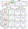 |
Fig. A.1 Top: correction factors |
![Mathematical equation: \hbox{${F = \dot{R}_{\rm rim}/ V_{\rm peak\,sep.}^{\rm [N\,II]}}$}](/articles/aa/full_html/2018/01/aa31788-17/aa31788-17-eq307.png)
![Mathematical equation: \hbox{${F^* = \dot{R}_{\rm shell}/ V_{\rm peak\,sep.}^{\rm [N\,II]}}$}](/articles/aa/full_html/2018/01/aa31788-17/aa31788-17-eq308.png)
![Mathematical equation: \hbox{${F^* = \dot{R}_{\rm shell}/ V_{\rm peak sep.}^{\rm [N\,II]}}$}](/articles/aa/full_html/2018/01/aa31788-17/aa31788-17-eq310.png)
Appendix B: Difference images
Here we present all the difference images used in this work for illustrating the magnification process. The case of IC 418 is shown in Fig. 1.
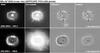 |
Fig. B.1 Magnification process for BD +30°3639. In the left two columns, the images in [O iii] and [N ii] are shown. The third column shows the simple difference in corresponding [O iii] and [N ii] images from the two epochs (shown in the image headers). White-black difference patterns are the signatures of global growth between epochs. The residuals (fourth column) are similar to the difference images except that the earlier image was magnified by a factor M before the images were subtracted. The value of M is determined (by trial and error) to null the residual image as much as possible. |
All Tables
Our adopted expansion distances, Dexp, and comparisons with other determinations.
Luminosities and corresponding masses estimated from post-AGB evolutionary tracks for our sample of Galactic disk central stars with determined expansion distances.
All Figures
|
Fig. 1 Example of the magnification process for IC 418. Shown are the images in [O iii] and [N ii] (left two columns). The third column shows the signal of expansion, and the fourth shows the difference after the first-epoch image was magnified by a factor M before subtraction (see text for more details). Corresponding sets of images for the other targets are found in Appendix B. |
| In the text | |
|
Fig. 2 Snapshot of a hydrodynamical PN model (left column) and comparison with observable quantities like [O iii] λ 5007 Å surface brightness (top right) along the minor axis and central line profile (bottom right) of IC 2448. Symbols are the observations, solid lines the model predictions. The model is from a sequence introduced in Steffen & Schönberner (2006, Fig. 6, right panel which utilizes the “revised” wind model of Pauldrach et al. (2004). The parameters of the model are given in the legend. The PN model proper extends from 1.5 × 1017 cm to 5 × 1017 cm, consisting of a high-density part, the “rim”, and a low-density part, the “shell”, both embracing the shock-heated “bubble” (cavity). The top left panel gives also the ion density distribution (total, He2+, O2+, N+), the middle panel: the radial velocity field, and the bottom panel: the electron temperature. The two tiny temperature spikes indicat the leading shocks of rim and shell, respectively. The shell engulfs halo matter (former AGB wind) where the history of the final AGB evolution is stored, and the rim engulfs the slower upstream matter of the shell. The weak appearance of the shell as seen in the surface brightness and line profile reflects the density difference between rim and shell, although most of the nebular mass (up to about 80%) resides within the shell. |
| In the text | |
|
Fig. 3 Ratios of measured rim and shell expansion timescales (kinematical ages), i.e. |
| In the text | |
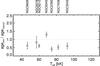 |
Fig. 4 Same as in Fig. 3, but now rim ages over microstructure ages; data again from Table 2. |
| In the text | |
|
Fig. 5 Ratio |
| In the text | |
|
Fig. 6 Distances from [N ii] images vs. distances from [O iii] images for objects with measurements in both filters. Open squares are for shell (3) and filled square for rim measurements (7). |
| In the text | |
|
Fig. 7 Comparison of shell and rim distances for the three objects for which reliable shell data exist (cf. Tables 4 and 5). Open symbols are for [O iii], filled for [N ii]. |
| In the text | |
|
Fig. 8 Distances according to Frew et al. (2016) vs. our expansion distances; data from Table 7. Objects mentioned in the text are labelled. The dotted line is the 1:1 relation. |
| In the text | |
|
Fig. 9 Same as in Fig. 8, but for the Stanghellini & Haywood (2010) calibration. |
| In the text | |
|
Fig. 10 Same as in Fig. 8, but for the spectroscopic (gravity) distances of Méndez et al. (1992), MKH (squares), Pauldrach et al. (2004), PHM (circles), and Kudritzki et al. (2006), KUP (diamonds). There are up to three spectroscopic distance per object. |
| In the text | |
|
Fig. 11 HRD of PNe nuclei together with evolutionary tracks of hydrogen-burning AGB remnant after Miller Bertolami & Althaus (2006, priv. comm., solid). Numbers at the tracks denote the central-star masses in solar units. Tracks of AGB remnants from Blöcker (1995) and Schönberner (1983) are also shown (dashed) for comparison. Their masses are (from bottom to top): 0.553, 0.565, 0.605, and 0.696 M⊙, respectively. The 0.517 and 0.553 M⊙ remnants start their post-AGB evolution as burning helium. The upward “hooks” are due to the rekindling of hydrogen which then slows down the evolution considerably. The filled circles with the respective error bars mark the positions of the Milky Way disk objects listed in Table 8. We show also nine (hydrogen-rich) objects from the Magellanic Clouds (seven from the Large Cloud, circles, and two from the Small Cloud, squares), taken from the analyses of Herald & Bianchi (2004) and Herald & Bianchi (2007). Also, five objects from the Milky Way bulge with the parameters derived by Hultzsch et al. (2007) are displayed (diamonds). The position of K648 in M 15 is based on the recent study of Jacoby et al. (2017). |
| In the text | |
|
Fig. A.1 Top: correction factors |
| In the text | |
|
Fig. B.1 Magnification process for BD +30°3639. In the left two columns, the images in [O iii] and [N ii] are shown. The third column shows the simple difference in corresponding [O iii] and [N ii] images from the two epochs (shown in the image headers). White-black difference patterns are the signatures of global growth between epochs. The residuals (fourth column) are similar to the difference images except that the earlier image was magnified by a factor M before the images were subtracted. The value of M is determined (by trial and error) to null the residual image as much as possible. |
| In the text | |
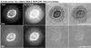 |
Fig. B.2 Same as Fig. B.1, but for IC 2448. |
| In the text | |
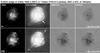 |
Fig. B.3 Same as Fig. B.1, but for IC 4593. |
| In the text | |
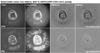 |
Fig. B.4 Same as Fig. B.1, but for NGC 2392. |
| In the text | |
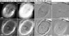 |
Fig. B.5 Same as Fig. B.1, but for NGC 3132. |
| In the text | |
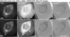 |
Fig. B.6 Same as Fig. B.1, but for NGC 3242. |
| In the text | |
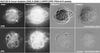 |
Fig. B.7 Same as Fig. B.1, but for NGC 3918. |
| In the text | |
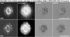 |
Fig. B.8 Same as Fig. B.1, but for NGC 5882. |
| In the text | |
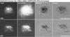 |
Fig. B.9 Same as Fig. B.1, but for NGC 6210. |
| In the text | |
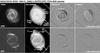 |
Fig. B.10 Same as Fig. B.1, but for NGC 6543. |
| In the text | |
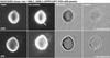 |
Fig. B.11 Same as Fig. B.1, but for NGC 6565. |
| In the text | |
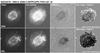 |
Fig. B.12 Same as Fig. B.1, but for NGC 6578. |
| In the text | |
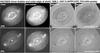 |
Fig. B.13 Same as Fig. B.1, but for NGC 6826. |
| In the text | |
 |
Fig. B.14 Same as Fig. B.1, but for NGC 6886. |
| In the text | |
 |
Fig. B.15 Same as Fig. B.1, but for NGC 6891 ([O iii] only). |
| In the text | |
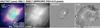 |
Fig. B.16 Same as Fig. B.1, but for NGC 7027. |
| In the text | |
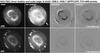 |
Fig. B.17 Same as Fig. B.1, but for NGC 7662. |
| In the text | |
Current usage metrics show cumulative count of Article Views (full-text article views including HTML views, PDF and ePub downloads, according to the available data) and Abstracts Views on Vision4Press platform.
Data correspond to usage on the plateform after 2015. The current usage metrics is available 48-96 hours after online publication and is updated daily on week days.
Initial download of the metrics may take a while.