| Issue |
A&A
Volume 609, January 2018
|
|
|---|---|---|
| Article Number | A102 | |
| Number of page(s) | 16 | |
| Section | Extragalactic astronomy | |
| DOI | https://doi.org/10.1051/0004-6361/201731592 | |
| Published online | 23 January 2018 | |
Inner and outer star forming regions over the disks of spiral galaxies
I. Sample characterization⋆
1 Departamento de Física Teórica, Universidad Autónoma de Madrid, 28049 Madrid, Spain
2 Instituto Nacional de Astrofísica, Óptica y Electrónica, Luis E. Erro 1, 72840 Tonantzintla, Puebla, Mexico
e-mail: This email address is being protected from spambots. You need JavaScript enabled to view it.
3 Instituto de Astronomía, Universidad Nacional Autónoma de México, A.P. 70-264, 04510 México D.F., Mexico
Received: 18 July 2017
Accepted: 18 October 2017
Abstract
Context. The knowledge of abundance distributions is central to understanding the formation and evolution of galaxies. Most of the relations employed for the derivation of gas abundances have so far been derived from observations of outer disk H ii regions, despite the known differences between inner and outer regions.
Aims. Using integral field spectroscopy (IFS) observations we aim to perform a systematic study and comparison of two inner and outer H ii regions samples. The spatial resolution of the IFS, the number of objects and the homogeneity and coherence of the observations allow a complete characterization of the main observational properties and differences of the regions.
Methods. We analyzed a sample of 725 inner H ii regions and a sample of 671 outer H ii regions, all of them detected and extracted from the observations of a sample of 263 nearby, isolated, spiral galaxies observed by the CALIFA survey.
Results. We find that inner H ii regions show smaller equivalent widths, greater extinction and luminosities, along with greater values of [N ii] λ6583/Hα and [O ii] λ3727/[O iii] λ5007 emission-line ratios, indicating higher metallicities and lower ionization parameters. Inner regions have also redder colors and higher photometric and ionizing masses, although Mion/Mphot is slighty higher for the outer regions.
Conclusions. This work shows important observational differences between inner and outer H ii regions in star forming galaxies not previously studied in detail. These differences indicate that inner regions have more evolved stellar populations and are in a later evolution state with respect to outer regions, which goes in line with the inside-out galaxy formation paradigm.
Key words: methods: data analysis / techniques: imaging spectroscopy / galaxies: spiral / Hii regions
Table 4 is only available at the CDS via anonymous ftp to cdsarc.u-strasbg.fr (130.79.128.5) or via http://cdsarc.u-strasbg.fr/viz-bin/qcat?J/A+A/609/A102
© ESO, 2018
1. Introduction
It is widely recognized that the knowledge of abundance distributions in galaxies is very important as a probe of their chemical evolution and star formation histories. H ii regions in external spiral and irregular galaxies provide an excellent means to derive the chemical abundances of different elements, both primordial and product of stellar nucleosynthesis. This information is central to guiding theoretical models of the formation and evolution of galaxies.
Among the different abundance-related parameters employed are: (i) the radial metallicity gradient; (ii) the average metallicity at a given fiducial galactic radius; and (iii) the central metallicity value, where the term “metallicity” usually refers to oxygen abundance, oxygen being the most abundant element in the universe after hydrogen and helium. In fact, the two latter parameters rely on the determination of the first, since they are calculated either by interpolation or extrapolation of the metallicity distribution respectively. However, it should be kept in mind that what is referred to as “abundance” or “radial abundance gradient” of a galaxy in fact represents an observational limitation derived from the need to use fixed aperture and/or long-slit spectroscopy. The information actually required to deeply approach the issue of the formation and evolution of disk galaxies is the map of the abundance distribution of the different elements, that up to now represented a very difficult and highly time consuming task. New multi-slit and integral field spectroscopy (IFS) data are now readily obtained, which have greatly increased the number of H ii regions analyzed per given galaxy, although our methodologies still suffer from essentially the same systematic uncertainties in the determination of gas abundance distributions.
In general terms, there are two different approaches to derive elemental gas abundances: the so called direct method, which makes use of the measurement of the electron temperature Te from the quotient of (faint) auroral to (strong) nebular lines of different elements (O, N, and S among others), and semi-empirical models, in which combinations of (strong) nebular lines are used to infer abundances in regions where the (faint) auroral lines cannot be detected through suitable calibrations. Due to the cooling properties of the nebulae, the regions to which the direct method is applicable are of low metallicity and therefore, in the case of spiral galaxies, tend to reside in the outer disc zones, while the regions that require the application of semi-empirical methods, being of higher metallicity, tend to reside in the most inner zones of the discs. These different treatments of outer and inner disc H ii regions can complicate the interpretation of the radial gas abundance gradients, and could even produce artificial effects if inner and outer H ii regions differ in physical properties and ionization structure.
Although the emission line spectra of H ii regions in the inner and outer regions of disks look alike, some differences between these two families are recognized. Inner H ii regions seem to show lower [O iii] λ5007/Hβ values than their outermost counterparts, an effect that can be produced by the combination of lower effective temperatures of their ionizing stars, higher dust content and higher metallicity; at the same time, [O ii] λ3727/[O iii] λ5007 is higher in the spectra of the inner regions, which seems to indicate a lower excitation of the gas; [N ii] λ6583/[O ii] λ3727 is also higher, pointing to a larger N/O, also indicative of a higher overall metallicity (Perinotto 1983). A hint of somewhat higher electron density of the emitting gas in the inner regions has also been reported (Kennicutt et al. 1989; Bresolin et al. 2004; Díaz et al. 2007). At high abundances, as those expected for inner or circumnuclear H ii regions, the density of the nebula affects significantly the strength of emission lines, specially [O iii], due to the competition between collisional and radiative de-excitation in the nebular cooling fine structure O++ transitions (Oey & Kennicutt 1993).
Higher extinctions, such as could be expected in higher metallicity and higher density regions, could also have an impact on the emission line intensities. The presence of dust can modify the thermal structure of nebulae in several ways. Firstly, the removal of cooling agents from the gas phase via depletion onto grains will increase the electron temperature (Henry 1993). Secondly, dust grains can absorb a given fraction of the Lyman continuum photons and thus modify the ionizing radiation field (Mathis 1986). The absorbed energy will then be re-radiated in the IR (Mas-Hesse & Kunth 1991). Heating or cooling by photo-emission or recombination from charged grains can also affect the thermal balance of the nebulae (Baldwin et al. 1991).
There is no doubt that the analysis of high excitation, low metallicity spectra is easier than that of the opposite case, and the larger contribution from the underlying stellar continuum in the case of the innermost regions represents a limitation. Therefore, despite any inferred different physical properties of inner and outer H ii regions, most of the relations currently employed for the derivation of abundances have been derived from observations of outer disk regions and have been assumed to be valid for all the ionized regions over the whole galactic disk. On the other hand, these inferences have been obtained from the study, albeit detailed, of a relatively small number of objects.
Fortunately it is now possible with the advent of multi-object spectrographs (MOS) or integral field units (IFU) to perform a complete spectroscopic mapping of the distributions of H ii regions over the disks of spirals (see e.g., Rosolowsky & Simon 2008; Rosales-Ortega et al. 2011; Bresolin & Kennicutt 2015). A brief account of the results of this kind of work includes the presence of a considerable dispersion in the derived abundances at a given galactocentric distance and the indication of possible azimuthal variations. The first could be due to the different sizes of the H ii regions observed, with the smallest regions being affected by stochasticity in the stellar mass function, and the second could be ascribed to differences in star formation in and between spiral arms and also to differences in mixing in the turbulent interstellar medium.
The recently completed Calar Alto Legacy Integral Field Area (CALIFA) survey provides an excellent opportunity to perform a systematic study of the properties of inner and outer H ii regions over the disks of spiral galaxies, since the homogeneity of the data regarding both observations and handling is a requirement to obtain reliable results. This in turn will give us the possibility of exploring the effects that any existing differences may have in derived properties of the regions themselves, such as elemental abundances, ionization structure, evolutionary state, amongst other.
This is the first article of a series and presents the account of the observational properties of inner and outer regions in a sample of 263 nearby, isolated, spiral galaxies. In Sect. 2 we provide a summary of the observations on which the work is based. Section 3 presents the characteristics of both the galaxy sample and the H ii region sample used. Section 4 presents the results of this characterisation, together with their discussion. Finally our conclusions are summarized in Sect. 5.
Physical properties of part of the CALIFA galaxies involved in this work, as described in the text.
2. Summary of observations and data reduction
The galaxies used in this work are part of the CALIFA project, one of the most ambitious 2D-spectroscopic surveys to date. The observations were carried out at the Centro Astronómico Hispano-Alemán (CAHA) 3.5 m telescope. This work is based on the 350 galaxies observed using the low-resolution setup until September 2014. Most of these galaxies are part of the 2nd CALIFA Data Release (DR2; García-Benito et al. 2015), and therefore the datacubes are accessible from the DR2 webpage1. The CALIFA survey is already finished, and the complete observations are included in the CALIFA final data (DR3; Sánchez et al. 2016a).
The details of the survey, sample, observational strategy, and data reduction are explained in Sánchez et al. (2012a). All galaxies were observed using the Postdam Multi Aperture Spectrograph (PMAS; Roth et al. 2005) in the PPAK configuration (Verheijen et al. 2004; Kelz & Roth 2006; Kelz et al. 2006), that is, a retrofitted bare fibre bundle IFU which expands the field-of-view (FoV) of PMAS to a hexagonal area with a footprint of 74 × 65 arcsec2, which allows us to map the full optical extent of the galaxies up to two to three disk effective radii on average. This is possible because of the diameter selection of the sample (Walcher et al. 2014; hereafter W14). The observing strategy guarantees a complete coverage of the FoV, with a final spatial resolution of full width at half maximum (FWHM) ~3′′, corresponding to ~1 kpc at the average redshift of the survey. The sampled wavelength range and spectroscopic resolution (3745–7500 Å, λ/△ λ ~ 850 for the low-resolution setup, that we use in this work) are more than sufficient to explore the most prominent ionized gas emission lines and to deblend and subtract the underlying stellar population (e.g., Sánchez et al. 2012a; Kehrig et al. 2012; Cid Fernandes et al. 2013). The dataset was reduced using version 1.5 of the CALIFA pipeline. The flux calibration, signal-to-noise ratio (S/N) and related uncertainties of the CALIFA data products have been thoroughly discussed in several articles of the CALIFA collaboration (e.g., Sánchez et al. 2012a; Cid Fernandes et al. 2014; García-Benito et al. 2015). For the 1st CALIFA Data Release (DR1; Husemann et al. 2013) the collaboration performed a data quality test showing that the sample reached a median limiting continuum sensitivity of 10-18 erg s-1 cm-2 Å-1 arcsec-2 at 5635 Å, and 2.2 × 10⁻¹⁸ erg s-1 cm-2 Å-1 arcsec-2 at 4500 Å, for the V500 and V1200 setup respectively, which corresponds to limiting r- and g-band surface brightnesses of 23.6 mag arcsec-2 and 23.4 mag arcsec-2, or an unresolved emission-line flux detection limit of roughly 10-17 erg s-1 cm-2 arcsec-2 and 0.6 × 10⁻¹⁷ erg s-1 cm-2 arcsec-2, respectively. The same limits, or slight improvements, were found in posterior data releases.
3. Sample characterization
3.1. Galaxy sample
The starting point of this work were the 350 CALIFA galaxies observed using the low-resolution setup until September 2014. From this initial sample we selected the spiral galaxies and discarded ellipticals and lenticulars, that have no gas and do not host big processes of stellar formation. We also selected those spirals that are isolated, as our objective is analyzing H ii regions not affected by particular processes of interactions or mergers. Combining the isolated and merging classification and the morphological type designation from the CALIFA survey with the Hyperleda2 catalog (Makarov et al. 2014) classification as a matter of extra precaution, we finally selected 263 galaxies, that from now on constitute the main sample of our work.
The main properties and characteristics of the 263 galaxies are included in Table 4, only available at the CDS. A part of this table is shown as an example in Table 1.
As it was important to ensure that the properties and parameter ranges of the 263 galaxies fulfilled the statistical properties of the whole CALIFA sample, with the only exception of the exclusion of the earlier morphological types, some of the main characteristics of the galaxies are particularly described in the following sections.
3.1.1. Redshifts and distances
Redshift values of our galaxies are those given by the CALIFA survey, that obtained them from the SIMBAD database on January 2010 (W14). Our galaxy sample has a redshift range, shown in Fig. 1, that covers the whole range of redshift values selected by CALIFA for its mother sample (0.005 <z< 0.03).
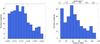 |
Fig. 1 Redshifts values (left) and of distance values in Mpc (right). Both histograms correspond to the galaxy sample of this work. |
Distances for the CALIFA mother sample were obtained from NED and Hyperleda, finally adopting the NED-infall-corrected ones as their fiducial distances. In this work we adopt the distances calculated from the distance moduli given by Hyperleda, which are corrected for Virgo-centric infall. The distance range for our galaxy sample is also included in Fig. 1, along with the scale range expresed in kpc/′′.
3.1.2. Morphological classification
We adopted the morphological classification performed by the CALIFA team (W14). The CALIFA collaboration found that the morphological classifications available from public databases were incomplete for the CALIFA sample (e.g., Galaxy Zoo 2, 535 matches; Willett et al. 2013) or missing a consistent classification in Hubble subtypes (NED). Therefore they undertook their own reclassification, using human by-eye classification (see W14).
One of the defining characteristics of CALIFA mother sample is that it contains galaxies of all morphological types. In our case we only have spirals by selection, but our sample also comprises galaxies of all spiral morphological types. The morphological type histogram of our sample (Fig. 2) follows a similar pattern in the Sa-Sm types that the one we can observe in the analogous histogram of the CALIFA mother sample (see W14).
Regarding the presence of bars and rings, using the classification by Hyperleda we find a 40.3% of barred galaxies in our sample, and a 17.1% of galaxies where the presence of a ring can be observed.
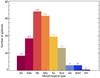 |
Fig. 2 Distribution of morphological types for the galaxy sample of this work. |
3.1.3. Inclination
As described in W14, inclination may be the cause of a selection effect in the CALIFA mother sample, and thus in ours. Isophotal sizes of flattened, transparent (no attenuation) galaxies vary with inclination, due to the projected change of surface brightness (e.g., Opik 1923). It is therefore easier for an inclined disk galaxy to get into a sample defined by a minimum apparent isophotal size than it is for a face-on system of the same intrinsic dimensions. The magnitude of this effect depends on the degree of transparency; it is strongest for a fully transparent galaxy, and it disappears when the system is opaque, so that only its surface is observed. Therefore it can be expected to find an excess of galaxies with high inclinations in the CALIFA sample, at least among disk-dominated systems, and this may happen also in the spiral sample of this work.
During the characterization of their mother sample, the CALIFA team detected this effect when studying isophotal major and minor axes delivered by the SDSS photometric pipeline, that can be combined into an axis ratio at the outer 25 mag/arcsec2 level (see W14). They found that the histogram of isophotal axis was clearly skewed toward low values of b/a, providing an indication of the considered selection effect. Furthermore, they also represented the 55 galaxies of the CALIFA mother sample that have Mr> −18.6, that is, that are below the completeness limit. Nearly all of these galaxies have axis ratios below 0.4, and it can be visually confirmed that these are predominantly disk-dominated systems that are close to edge-on. The CALIFA team presumed that very few, if any, of these galaxies would have been included into the CALIFA sample of seen face-on, their angular sizes have been boosted through inclination, just enough to promote them into the sample. They reached the conclusion that while the CALIFA sample has a higher proportion of inclined disk galaxies at the faint end, the overall effect is not large. Specifically for the galaxies close to and below the low-luminosity completeness limit there is at any rate a clear surplus of galaxies with very high inclinations in the CALIFA sample.
We derive the inclination values for our galaxy sample from the b/a axis ratios given by CALIFA, that obtained them by calculating light moments. The final b/a value is the mean of the axis ratios of ellipses containing 50% and 90% of the total flux (see W14). To obtain the final inclination values we use the expression given by Holmberg (1958), where the value of the axial ratio for an edge-on system parameter as a function of the galaxy morphological type is given by Heidmann et al. (1972). In Fig. 3 we represent the inclination values for the whole sample and also for the 31 galaxies that are below the CALIFA completeness limit. We find a distribution skewed toward high inclination values, that is more prominent for the faint galaxies. We consider therefore that we are detecting the selection effect already existing in the CALIFA mother sample, and that specifically affects galaxies with low luminosity.
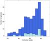 |
Fig. 3 Inclination values for this work galaxy sample, calculated from the observed axis ratios. Values of all galaxies are represented in dark blue, and overplotted in light blue are the values of the galaxies with Mr> −18.6. |
This high number of high inclination or edge-on galaxies have to be taken into account, as it implies that these galaxies will have higher uncertainties in the determination of the distances of their star forming regions to the center of the system, as well as it can affect the morphological classification and other factors.
3.1.4. Effective radius
In this work we used the disk effective radius, classically defined as the radius at which one half of the total light of the system is emitted, as the factor of normalization to analyse the galaxy properties’ radial distributions and compared them galaxy to galaxy. Concerning the study of radial gradients and 2D distribution of galactic properties, although there are a high number of studies about the issue, we find a large degree of discrepancy among them. One of the factors that may cause these differences is the fact that it does not exist an uniform method to analyse the gradients. In some cases the physical scales of the galaxies (i.e., the radii in kpc) are used (e.g., Marino et al. 2012). In others the scale-lengths are normalized to the R25 radius, that is, the radius at which the surface brightness in the B band reach the value of 25 mag/arcsec2 (e.g., Rosales-Ortega et al. 2011). Finally, a reduced number of studies try to normalize the scale-length based on the effective radii. Díaz (1989) already showed that the effective radius seems to be the best to normalize the abundance gradients. Using the physical scale of the radial distance or the normalized one to an absolute parameter like the R25 radius does not produce gradients that we can compare galaxy to galaxy, since in both cases the derived gradient is correlated with either the scale-length of the galaxy or its absolute luminosity.
We used the effective radii values estimated by the CALIFA survey, whose calculation is described in Sánchez et al. (2012b). It is based on an analysis of the azimuthal surface brightness profile, derived from an elliptical isophotal fitting of the ancillary g-band images collected for the galaxies (extracted from the SDSS imaging survey, York et al. 2000; Mármol-Queraltó et al. 2011). When these ancillary images were not available, the B band was used (Mármol-Queraltó et al. 2011). Our galaxy sample contains a wide range of effective radii, as shown in Fig. 4, wich implies that we selected galaxies with a wide range of sizes.
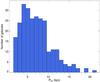 |
Fig. 4 Effective radius values (kpc) of this work galaxy sample. |
3.1.5. Color–magnitude diagrams
The color–magnitude diagram of the 263 galaxies of our sample, represented in Fig. 5, show that they fully cover the range in absolute magnitudes where the CALIFA sample is representative of the overall galaxy population. This is consistent with the results obtained by Schawinski et al. (2014), that signaled the fact that late-type galaxies do not separate into a blue cloud and a red sequence, but rather span almost the entire color range without any gap or valley.
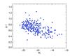 |
Fig. 5 Distribution of this work galaxy sample in the g−r vs. Mr color–magnitude diagram. |
3.2. Spectroscopic information of the HII regions sample
The H ii region segregation and their corresponding spectra extraction is performed using a semi-automatic procedure named HIIexplorer, described in Sánchez et al. (2012b) and Rosales-Ortega et al. (2012). It is based on the assumptions that: (a) H ii regions are peaky and isolated structures with a strong ionized gas emission, which is significantly above the stellar continuum emission and the average ionized gas emission across the galaxy. This is particularly true for Hα because (b) H ii regions have a typical physical size of about a hundred or a few hundred parsecs (e.g., González Delgado & Pérez 1997; Lopez et al. 2011; Oey et al. 2003), which corresponds to a typical projected size of a few arcsec at the distance of the galaxies. These basic assumptions are based on the fact that most of the Hα luminosity observed in spiral and irregular galaxies is a direct tracer of the ionization of the interstellar medium (ISM) by the ultraviolet (UV) radiation produced by young high-mass OB stars. Since only high-mass, short-lived stars contribute significantly to the integrated ionizing flux, this luminosity is a direct tracer of the current star formation rate (SFR), independent of the previous star formation history. Therefore, clumpy structures detected in the Hα intensity maps are most probably associated with classical H ii regions (i.e., those regions for which the oxygen abundances have been calibrated).
For each region selected by HIIexplorer, we extracted a integrated spectrum of the spaxels belonging to that region. For each individual extracted spectrum we then modeled the stellar continuum using FIT3D, a fitting package described in Sánchez et al. (2006) and Sánchez et al. (2011). The FIT3D version used at the moment of this fitting adopted a simple SSP template grid with 12 individual populations. It comprises four stellar ages (0.09, 0.45, 1.00, and 17.78 Gyr), two young and two old ones, and three metallicities (0.0004, 0.019, and 0.03, that is, subsolar, solar, or supersolar, respectively). The models were extracted from the SSP template library provided by the MILES project (Vazdekis et al. 2010; Falcón-Barroso et al. 2011). The Cardelli et al. (1989) law for the stellar dust attenuation with an specific attenuation of RV = 3.1 was adopted, assuming a simple screen distribution.
Individual emission line fluxes were measured in the stellar-population subtracted spectra performing a multicomponent fitting using a single Gaussian function. The equivalent widths for each H ii region and line were estimated using the results from the fitting analysis instead of the classical procedure, by dividing the emission line integrated intensities by the underlying continuum flux density. The continuum was estimated as the median intensity in a bandwidth of 100 Å, centered in the line, using the gas-subtracted spectra provided by the fitting procedure. For further details about both processes, see Sánchez et al. (2012b). The errors in the determination of the emission line fluxes and their reliability are discussed extensively in Sánchez et al. (2016b and c) for the Pipe3D/FIT3D fitting technique.
After applying all the process to the 263 CALIFA galaxies datacubes, we detected a total of 12 891 H ii regions. Nevertheless, not all these regions can be accepted as confirmed H ii regions due to the high level of noise of some spectra or the non-physical values of some parameters such as Hα/Hβ. Therefore we apply a quality control process, considering the following criteria to ensure that we are working with physical bona fide H ii regions and avoid selection uncertainties: (i) EW(Hα) > 6 Å, following Cid Fernandes et al. (2010), Sánchez et al. (2015); (ii) Hα/Hβ> 2.7. We consider the theoretical value for the intrinsic line ratio Hα/Hβ from Osterbrock & Ferland (2006), assuming case B recombination (optically thick in all the Lyman lines), an electron density of ne = 100 cm-3 and an electron temperature of Te = 104 K. Lowering the electron temperature to 5000 K, keeping the electron density constant, increases the Balmer decrement Hα/Hβ by a factor of 1.05 and translates to an uncertainty of 0.04 dex in c(Hβ) for the reddening curve employed. We also have included a certain margin to account for uncertainties in the observational values of the emission lines; (iii) Hα/Hβ< 6. This value corresponds to an extinction of ~2.3 mag. We consider that beyond this point values are not physical; (iv) F(Hβ) > 0.5 × 10⁻¹⁶ erg s-1 cm-2. To avoid lines with very small S/N; (v) F([O iii] λ5007)> 0.5 × 10⁻¹⁶ erg s-1 cm-2. This condition was introduced due to non-physical values of the [O iii] λ5007/Hβ emission-line ratio observed for some regions in a preliminar version of the data. We finally obtained a sample of 9281 selected H ii regions.
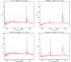 |
Fig. 6 Some of the inner regions extracted spectra, before the subtraction of the stellar continuum. Galaxy name, ID of the region in the galaxy and distance to the center are shown in the titles. Flux is expressed in units of 10-16 erg s-1 cm-2. |
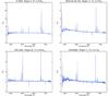 |
Fig. 7 Some of the outer regions extracted spectra, before the subtraction of the stellar continuum. Galaxy name, ID of the region in the galaxy and distance to the center are shown in the titles. Flux is expressed in units of 10-16 erg s-1 cm-2. |
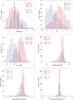 |
Fig. 8 From top to bottom and left to right: equivalent width of Hα, dust attenuation, Hα luminosity and of the [N ii] λ6583/Hα, [O ii] λ3727/[O iii] λ5007, and [S ii] λ6717/[S ii] λ6731 emission-line ratios for the inner (red diagonally-hatched diagram) and outer (blue horizontally-hatched diagram) region samples. |
3.2.1. Inner regions sample
We considered as inner regions those that fulfil the criterium established by Álvarez-Álvarez et al. (2015), based on the observed separation between nuclear and disk region rings as a function of the galaxy luminosity. Following this criterium, inner regions are those located closer to the center than the distance defined by the expression:  (1)We calculated the B-band magnitude from the g and r magnitudes from SDSS, using the transformation given by Lupton (2005)3. After applying this criterium to the primary regions sample we obtained a total of 794 inner regions. Nevertheless, by detailed examination of the region extracted spectra we note that not all the regions have clear visible emission from other typical H ii region spectral lines, apart from Hα. This could be previously expected, due to the strong stellar continuum found in the inner part of the galaxies, which prevents the detection of weaker spectral lines. Therefore we made a second selection process by examination by-eye, discarding those regions whose spectra were dominated by stellar continua with the presence of only weak Halpha emission, or by some gas emission features not clearly detectable. After that we obtained a final sample of 725 regions with spectra where Hα, Hβ, [O iii] λ5007, [N ii] λλ6548, 6583 or the [S ii] λ6717, 6731 doublet are measurable.
3.2.2. Outer regions sample
We considered as external H ii regions those that are located at a distance larger than two effective radii (Reff) from the center of the galaxy. It is around this radius where a certain amount of flatness is found in abundance gradients in spirals (Díaz 1989; Sánchez et al. 2014; Marino et al. 2016; Sánchez-Menguiano et al. 2016). From the primary sample of 9281 regions obtained, a total of 1027 regions were located beyond the considered distance to the center of the system. Nevertheless, as happened with the inner regions, not all of them show H ii region emission features or do not have a high enough S/N. We therefore applied a second selection by eye, obtaining a final sample of 671 inner regions.
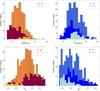 |
Fig. 9 Left column: EW(Hα) and AV histograms from the inner H ii regions sample as a function of their galaxies morphological types. Regions with Sa, Sab and Sb type galaxies are colored in dark red, those with Sbc, Sc and Scd type galaxies in orange and those with Sd, Sdm and Sm type galaxies are colored in gold. EW(Hα) is expressed in units of Å and AV in magnitudes. Right column: histograms with the same parameters as those from the outer H ii regions sample. Regions with Sa, Sab and Sb type galaxies are colored in dark blue, those with Sbc, Sc and Scd type galaxies in blue and those with Sd, Sdm and Sm type galaxies are colored in light blue. |
4. Results and discussion
4.1. Observational and functional parameters
After the process of extraction and selection we get a final sample of 725 inner regions and 671 outer regions. Some of the inner regions spectra are shown as an example in Fig. 6, while some of the outer region spectra are shown in Fig. 7.
The number of inner and outer regions included in the final samples allows us to develop a statistical analysis of some spectroscopic properties, especially those based on the strongest detected emission lines, such as the following:
-
(i)
EW(Hα), the equivalent width of Hα, which is directly related to the fraction of very young stars in the region.
-
(ii)
AV, the dust attenuation, calculated using the Balmer decrement according to the reddening function of Cardelli et al. (1989), assuming R ≡ AV/E(B−V) = 3.1. Theoretical value for the intrinsic line ratio Hα/Hβ was considered as explained in Sect. 3.2.
-
(iii)
L(Hα), the Hα luminosity, obtained from the reddening-corrected Hα flux, considering the distances to the corresponding galaxies.
-
(iv)
[N ii] λ6583/Hα line ratio, related to the oxygen abundance of the ionized gas, and that along with the [O iii] λ5007/Hβ provides information about the nature of the ionization source of the region.
-
(v)
[O ii] λ3727/[O iii] λ5007 line ratio, related to the ionization parameter log u, a measurement of the strength of the ionization radiation (Díaz et al. 2000).
-
(vi)
[S ii] λ6717/[S ii] λ6731 line ratio, related to the electron density (ne) of the ionized gas.
Figure 8 shows EW(Hα), AV, L(Hα) and [N ii] λ6583/Hα, [O ii] λ3727/[O iii] λ5007, and [S ii] λ6717/[S ii] λ6731 emission-line ratio histograms for inner and outer region samples. Different trends and average values can be observed for both samples.
Firstly, EW(Hα) histograms show smaller EW(Hα) values for inner H ii regions. Sánchez et al. (2014), that work with a sample of 7016 H ii regions from 227 CALIFA galaxies also selected and extracted with HIIexplorer, finds a strong log-linear correlation between EW(Hα) and the percentage of young stars in the regions, obtained from the FIT3D fitting of the underlying stellar population. This correlation is valid for regions with EW(Hα) > 6 Å and with a percentage of young stars over 20%. All our regions have EW(Hα) over 6 Å, as it is one of our selection criteria. We consider the smaller values of EW(Hα) for our inner regions sample to be caused by the greater influence of the underlying stellar populations in those regions, and therefore to smaller percentages of young population (see Sect. 4.5). Secondly, on the middle histograms we observe larger AV values for inner regions, denoting greater dust attenuation. Finally, L(Hα) histograms reveal larger luminosities for inner regions. This is concordant with previous observations of very luminous H ii regions located close to their galactic nucleus (Álvarez-Álvarez et al. 2015), although it may be also influenced by a selection bias causing that in central regions, where the underlying continuum have a great influence, only the more luminous H ii regions can be detected. This possible selection bias will be studied afterwards in this section.
We find differences between the equivalent width and extinction values of inner regions as a function of the morphological type of the galaxies they belong to, as can be seen in Fig. 9. In early type spiral galaxies the greater prominence of the galaxy bulge implies greater influence of older underlying population, which means a decrease of the ionizing population percentage and of the equivalent width values. It also implies higher amounts of dust and therefore higher extinction values for these regions. On the contrary, late-type spirals, with little to none bulge component, have increasingly higher equivalent width values and less extinction. For the outer regions, differences between different morphological types are almost negligible.
Clear differences between inner and outer regions are also detected in histograms representing emission-line ratios, in Fig. 8. In the [N ii] λ6583/Hα histograms, at the top of the figure, we observe greater values for the inner regions. This emission-line ratio is related with the oxygen abundance, which is therefore higher in the inner regions, as could be expected for more evolved stellar populations and more enriched interstellar medium. Inner regions also have greater values of [O ii] λ3727/[O iii] λ5007 ratio, indicating in this case smaller values of the ionization parameter. In the case of [S ii] λ6717/[S ii] λ6731 histograms we find similar average values for outer and inner regions, corresponding to electron density values smaller than 10 cm-3 (Osterbrock & Ferland 2006). All the emission-line ratio histograms show sharper distributions for inner regions, while the outer regions are more scattered. This may be caused by lower uncertainties in the inner regions, whose spectra have higher S/N values.
Using the relation between the Hα luminosity and the number of ionizing Lyman continuum photons given by Gonzalez-Delgado et al. (1995) we calculate the number of ionizing photons for every H ii region. Results obtained for both inner and outer samples are shown in Fig. 10. Inner regions have higher values, as could be expected from their higher Hα luminosity values. As we have mentioned, this could be an intrinsic property or the result of a selection bias, caused by the fact the smaller inner regions are not detected due to the lack of spatial resolution and/or contrast with respect to the bright bulge. In order to study the magnitude of this possible bias we represent the histograms of the angular area in arcsec2 of the inner and outer regions, which are included in Fig. 11. We can see that although outer regions do, in fact, have a tail of smaller regions that is not present in the inner regions histogram (which is probably caused by this bias), the number of regions included in this tail is not enough to cause the difference of values ranges observed in the Hα luminosity and the number of ionizing photons histograms. Therefore we conclude that, although this selection bias has a small influence, there is an intrinsic difference of luminosity and number of ionizing photons between inner and outer H ii regions.
4.2. Systematics in diagnostic diagrams
Emission-line diagnostic diagrams (introduced by Baldwin et al. 1981; hereafter BPT) are a powerful way to study the nature of the dominant ionizing sources and changes in the physical conditions of the ionized nebulae, either from galaxy to galaxy, within each galaxy or within a particular nebulae. BPT diagrams work by exploring the location of certain line ratios, involving several strong emission lines with a dependence on the ionization degree and, to a lesser extent, on temperature or abundance. Through the application of different classification criteria (Kewley et al. 2001; Kauffmann et al. 2003) diagnostic diagrams allow the separation of galaxies or galaxy regions into those dominated by ongoing star formation and the ones dominated by non-stellar processes.
The distributions of CALIFA inner region sample and outer region sample in one of the most classical BPT diagrams, the [O iii] λ5007/Hβ vs. [N ii] λ6583/Hα diagram, are displayed in Fig. 12. In the case of the outer regions sample, data is color-coded according to their distance to the center of the galaxy bins that are indicated in the plot. It can be observed that the inner regions are mostly located to the bottom-right corner of the classical star forming branch, with the exception of a few regions located in the active galactic nuclei (AGN) zone demarcated by the Kewley et al. (2001) classification line, that will be analyzed afterwards. On the contrary, outer regions are more distributed along the star forming branch, and are generally located closer to the top-left corner. This is not surprising, as regions closer to the center of the galaxies are expected to have higher metallicities. Furthermore, Sánchez et al. (2014 and 2015) found a clear correlation reflected in their H ii regions distribution on the BPT diagrams, relating lower percentages of young stars with higher values of [N ii] λ6583/Hα. This is consistent with our results, as we would expect a larger contribution of the underlying stellar populations in the inner regions, and then lower percentage of young stars than in the outer regions.
We have studied the spectra of the H ii regions that, according to Kewley et al. (2001) classification criteria, are located in the AGN region of the BPT diagram in Fig. 12. In the case of the outer regions sample, we have five regions located in AGN zone, belonging to the galaxies IC 2101 (2 regions), IC 1528, UGC 09542 and UGC 09598. All the spectra have low S/N, with specifically very low values of the [O iii] λ5007 emission line. Considering this and the magnitude of the errors associated, we consider that the location of those regions in the AGN zone is due to the uncertainties associated to the emission line flux measurements.
In the case of the inner regions sample, we have six regions located in the AGN zone. Three of them are close to the classification line, while the other three are far inside the AGN region. These last three regions belong to the galaxies NGC 2410 and UGC 03973 (two regions). NGC 2410 is classified as a Seyfert 2 by NED (Véron-Cetty & Véron 2006) and UGC 03973 is classified as a Seyfert 1 by NED (Contini et al. 1998). Therefore we consider that the location of these regions in the AGN zone is due to their corresponding nucleus emission influence, and in fact the active nucleus emission features are easily detectable in their spectra. On the other hand, the other three regions belong to the galaxies IC 2247, UGC 00005 and UGC 03151, that are not classified as active. Their spectra have low S/N values and, as explained for the outer regions case, we consider that their location in the AGN regions is due to the uncertainties in the emission line measurements.
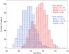 |
Fig. 10 Number of ionizing photons for the inner (red diagonally-hatched diagram) and outer (blue horizontally-hatched diagram) region samples. |
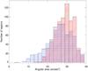 |
Fig. 11 Angular area in arcsec2 for the inner (red diagonally-hatched diagram) and outer (blue horizontally-hatched diagram) region samples. |
4.2.1. Observations of H ii regions with higher-spatial resolution
During the analysis of our CALIFA H ii regions sample we considered the possibility of including other IFS observations of H ii regions with higher-spatial resolution such as the sample extracted from the PPAK IFS Nearby Galaxy Survey (PINGS; Rosales-Ortega et al. 2010), in order to extend our data. While CALIFA galaxies have a redshift range of 0.005 < z < 0.03 (see Sect. 3.1.1), PINGS galaxies have much lower redshifts. This implies a loss of resolution that was studied by Mast et al. (2014) using some of the PINGS galaxies, that were simulated at higher redshifts to match the characteristics and resolution the galaxies observed by the CALIFA survey. Regarding the H ii region selection, the authors conclude that at z ~ 0.02 the H ii clumps can contain on average between one and six of the H ii regions obtained from the original data at z ~ 0.001. This prevents a complete combined analysis of CALIFA and PINGS regions, as parameters depending on the H ii regions size (luminosity, masses) are not comparable. Despite that, we can consider PINGS regions when analyzing properties where emission-line ratios are involved, that are independent of the size of the regions.
From a total sample of 17 nearby spiral galaxies included in the PINGS galaxy sample, we consider for this work those that are not involved in interaction or merging processes, as we did for the CALIFA galaxies. Our PINGS galaxy sample is therefore composed by four galaxies: NGC 628, NGC 1058, NGC 1637 and NGC 3184. Table 2 includes the main properties and characteristics of these four galaxies.
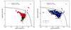 |
Fig. 12 Left: diagnostic diagram of the CALIFA inner region sample (red circles). Data from PINGS inner region sample (black diamonds), from CNSFR (green asterisks) studied by Díaz et al. (2007) and from central region (dark green triangle) of M33 studied by López-Hernández et al. (2013) are also included for comparison. Right: diagnostic diagram of the CALIFA outer region sample (blue circles). Different shades correspond to different bins of distance to the center of the galaxy, as indicated. Point from the IC 132 H ii region (orange square) of M33 studied by López-Hernández et al. (2013) is included for comparison. Overplotted as black lines in both diagrams are empirically and theoretically derived separations between LINERs/Seyferts and H ii regions. |
From the H ii regions catalog published by Rosales-Ortega (2009) we select those that fulfil our inner region criteria, specified in Sect. 3.2.1, obtaining a total of 79 inner regions, distributed along the four PINGS galaxies. The specific number of total and inner regions for each PINGS galaxy are indicated in Table 2. We obtain no outer regions from the PINGS galaxies, as their spatial linear coverage is smaller than the one of the CALIFA galaxies and no regions further than 2 Reff are extracted.
Physical properties of the PINGS galaxies involved in this work, obtained from the following sources.
The distribution of the PINGS inner region sample in the [O iii] λ5007/Hβ vs. [N ii] λ6583/Hα diagram, along with that from the CALIFA inner regions sample, is shown in Fig. 12. We can see that the PINGS inner regions follow the same pattern than the CALIFA inner regions: they have high [N ii] λ6583/Hα values, related to very high oxygen abundances and low percentages of young populations, and very low [O iii] λ5007/Hβ, due to low excitation values. The PINGS observations, with higher spatial resolution, allow the detection of inner regions located closer to their galaxy centers than CALIFA inner regions. Therefore the location of PINGS inner regions in the BPT diagram show the continuity of the trend already indicated by CALIFA inner regions.
The comparison with high-resolution circunmnuclear star forming region (CNSFR) observations, that go deeper in the high-metallicity, high-density region around the galactic nucleus, is also a case of great interest. (Díaz et al. 2007,hereafter D07) studied long-slit observations of 12 CNSFR located in the early-type spiral galaxies NGC 2903, NGC 3351 and NGC 3504. As in the case of PINGS observations, different spatial resolution prevents comparison between properties depending on the region sizes, but does not affect those properties related with the emission-line ratios. Data from these 12 CNSFR are included in the inner regions BPT diagram in Fig. 12, confirming the trend of high oxygen abundances and low excitation values.
An interesting case of IFS observations of H ii regions located in different environments is the study by (López-Hernández et al. 2013; hereafter LH13), that compares the central region of M33 with IC 132, a H ii region located at 19 arcmin (4.69 kpc) from the galactic center. These observations were obtained with the CAHA 3.5-m telescope, using the PMAS instrument in the PPAK mode, as were CALIFA and PINGS observations. Data from the central region and from IC 132 region are included in the corresponding inner and outer BPT diagrams in Fig. 12. While M33 central region confirms the high-metallicity, low-excitation values indicated by this work and by PINGS and Díaz et al. (2007) data, ID 132 region expand the trend of the outer regions, with lower metallicity and higher excitation.
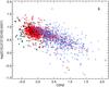 |
Fig. 13 Relation between [O ii] λ3727/[O iii] λ5007 emission-line ratio and the O3N2 index for the CALIFA inner (red diamonds) and outer (blue crosses) regions samples. Data from PINGS inner region sample (black stars), from CNSFR (dark green asterisks) studied by Díaz et al. (2007) and from central region (light green triangle) and IC 132 H ii region (orange square) of M33 studied by López-Hernández et al. (2013) are also included for comparison. |
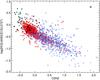 |
Fig. 14 Relation between [N ii] λ6583/[O ii] λ3727 emission-line ratio and the O3N2 index for the CALIFA inner (red diamonds) and outer (blue crosses) region samples. Data from PINGS inner region sample (black stars), from CNSFR (dark green asterisks) studied by Díaz et al. (2007) and from central region (light green triangle) and IC 132 H ii region of M33 (orange square) studied by López-Hernández et al. (2013) are also included for comparison. |
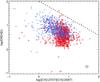 |
Fig. 15 Relation between EW(Hβ) and [O ii] λ3727/[O iii] λ5007 emission-line ratio for the inner (red diamonds) and outer (blue crosses) regions samples. Overplotted as a dashed black line is the relation given by Hoyos & Díaz (2006), explained in the text. |
4.2.2. Other diagnostic diagrams
The study of the relation between several emission-line ratios, that depend on the shape of the ionizing continuum and the physical conditions of the cloud, provide information on physical properties as ages, degree of ionization or abundances. The relation between the [O ii] λ3727/[O iii] λ5007 emission-line ratio and the O3N2 index, firstly introduced by Alloin et al. (1979) and defined as ![Mathematical equation: \begin{equation} {\rm O3N2}=\log \left(\frac{{\rm [O\,III]}\,\lambda5007/{\rm H}\beta}{{\rm [N\,II]}\,\lambda6584/{\rm H}\alpha}\right) , \end{equation}](/articles/aa/full_html/2018/01/aa31592-17/aa31592-17-eq58.png) (2)is shown in Fig. 13 for inner and outer CALIFA regions samples. We observe the existence of the same trend between both parameters for both outer and inner regions, although with a difference of one order of magnitude between their values. The O3N2 index, that has an inverse linear relation with the abundance, is smaller for inner regions, due to the weakness of the [O iii] λ5007 emission line in high metallicity regions. On the other hand outer regions have lower values of the [O ii] λ3727/[O iii] λ5007 emission-line ratio, denoting a higher degree of ionization than the inner regions sample. As only line ratios are involved and therefore the different spatial resolution has no influence, the PINGS inner regions sample is also included, as well as the CNSFR studied by D07 and M33 central and IC 132 regions studied by LH13. Their location in the plots confirms and expand the trend followed by the CALIFA inner and outer region samples, as was already seen in the BPT diagrams.
(2)is shown in Fig. 13 for inner and outer CALIFA regions samples. We observe the existence of the same trend between both parameters for both outer and inner regions, although with a difference of one order of magnitude between their values. The O3N2 index, that has an inverse linear relation with the abundance, is smaller for inner regions, due to the weakness of the [O iii] λ5007 emission line in high metallicity regions. On the other hand outer regions have lower values of the [O ii] λ3727/[O iii] λ5007 emission-line ratio, denoting a higher degree of ionization than the inner regions sample. As only line ratios are involved and therefore the different spatial resolution has no influence, the PINGS inner regions sample is also included, as well as the CNSFR studied by D07 and M33 central and IC 132 regions studied by LH13. Their location in the plots confirms and expand the trend followed by the CALIFA inner and outer region samples, as was already seen in the BPT diagrams.
Figure 14 shows the relation between the [N ii] λ6583/ [O ii] λ3727 emission-line ratio and the O3N2 index. The ratio [N ii]/[O ii] is a good metallicity indicator: with increasing metallicity the [O ii] decreases due to the decreasing electron temperature, that prevents the excitation of the O+ transition, while the [N ii] does not, therefore causing and increment in [N ii]/[O ii]. There is a good correlation between [N ii]/[O ii] and the N+/O+ ionic abundance ratio, which traces the nitrogen to oxygen abundance ratio (Pérez-Montero & Díaz 2005; Pérez-Montero & Contini 2009). This correlation was also found by D07 for high metallicity H ii regions and CNSFR. Results observed in Fig. 14 are in good agreement with in Figs. 12 and 13: inner regions have larger values of [N ii]/[O ii], according to their higher metallicity. As in the case of Fig. 13, the PINGS inner regions sample and the D07 and LH13 data are included in the figure, showing the same trend than the CALIFA inner and outer regions sample.
The relation between EW(Hβ) and [O ii] λ3727/[O iii] λ5007 emission-line ratio (see Fig. 15) provides information about the evolution of the star formation processes within a given galaxy. This line ratio is a proxy for the ionization parameter, which in turn is proportional to the quotient of the density of Ly continuum photons to the electron density. The number of hydrogen ionizing photons decreases with the evolution of the ionizing cluster and, other things being equal, lowers the ionization parameter, hence increasing the [O ii] λ3727/[O iii] λ5007 line ratio (Hoyos & Díaz 2006). The trend of decreasing EW(Hβ), and therefore increasing age for the ionizing population, and increasing [O ii] λ3727/[O iii] λ5007 line ratio can be seen in Fig. 15 for the observed regions up to EW(Hβ) around 3 Å. Below this value, which corresponds to ages of the H ii regions of about 10 Myr, we are seeing probably the contribution of an important underlying stellar population which decreases EW(Hβ) while keeping the ratio [O ii] λ3727/[O iii] λ5007 practically constant. The dashed line in the figure marks the envelope of the relation corresponding to the younger H ii region ages and the minimum underlying stellar population contribution (log EW(Hβ) = 2.00−0.73 log [O ii] λ3727/[O iii] λ5007 in Hoyos & Díaz (2006)). Ionizing clusters would beging their evolution from this line downwards, with the starting point depending on their initial mass (higher masses to the left in the plot). Outer regions show larger EW(β) values, related to younger ionizing stellar populations, and smaller [O ii] λ3727/[O iii] λ5007 values, implying larger ionization parameter values. Since, on average, inner H ii regions have Hα luminosities larger than outer ones by about an order of magnitude, this implies that, according to the previous description, the inner regions are ionized by more evolved clusters.
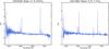 |
Fig. 16 Spectra from two of the ten H ii regions located further than 6 Reff from their galaxy center, before the subtraction of the stellar continuum. Galaxy name, ID of the region in the galaxy and distance to the center are shown in the titles. Flux is expressed in units of 10-16 erg s-1 cm-2. |
Physical properties of outer regions located further than 6 Reff from their galaxy center.
4.3. Furthest regions
The use of IFS techniques allows the detection of H ii regions located much further from the center of the galaxy than it was possible so far (see e.g., Ferguson et al. 1998; van Zee et al. 1998; Werk et al. 2010). In this work 10 of our 671 outer regions are located beyond 6 Reff, and although five of these ten regions are located close to the projected axis of high inclination galaxies, and therefore have high uncertainties in the determination of their distances to their galactic centers, we consider this group worthy of specific study. Two of these region spectra are included as an example in Fig. 16, and their most prominent properties are included in Table 3. Mean values of these properties for the whole outer H ii regions sample are also included in the table for comparison. These ten furthest regions were in fact already highlighted in the outer regions BPT diagram in Fig. 12, where it can be observed that they fulfil the general trend followed by the outer regions: they have low [N ii] λ6583/Hα emission-line ratio values and high [O iii] λ5007/Hβ emission-line ratio values, implying low oxygen abundances and high excitations. Other parameters, as EW(Hα), AV and L(Hα) also confirm the outer regions trends, as they are in general in good agreement with the outer region average values but slighty above or below, following the corresponding tendency observed in this work for the evolution of the parameter along the galactocentric distance.
4.4. Color-magnitude diagrams
Magnitudes and colors of the outer and inner H ii regions are calculated from their extracted spectra, for a first approach to the spectroscopic properties of the stellar populations. For the calculation of the magnitudes we followed the process indicated in Mollá et al. (2009) and García-Vargas et al. (2013). The filters we considered are the B and V bands from the Johnson’s system, and g and r bands from the Sloan SDSS ugriz system, as they are the ones comprised in our data wavelength range. The emission lines considered in the calculation are: [O ii] λ3727, Hγ, Hβ, [O iii] λ4959, [O iii] λ5007, He iλ5876, [O i] λ6300, [N ii] λ6548, Hα, [N ii] λ6583, [S ii] λ6717, and[S ii] λ6731. The transmission curves, the transmission values as a function of wavelength and the transmission values of the broadband filters at the rest wavelength of the selected emission lines employed are those included in the mentioned references. The magnitudes are calculated using the expression:  (3)where λ1 and λ2 are the passband limits in each filter, Lλ is the stellar SED luminosity, Li is the integrated luminosity in the narrow line for the line i and Ti the line filter transmission. We assumed that the line width is much narrower that the broadband filter passband. For Johnson’s filters, C is the constant for flux calibration in the Vega system. According to the Girardi et al. (2002) prescriptions, Vega is taken as the average of Lejeune et al. (1997) models for Z = 0.004 and Z = 0.008 at T = 9500 K (Vega’s data: Z = 0.006, mbol = 0.3319, BC = −0.25 and V = 0.58). C values are 3.27 for B (in this case, where we are calculating B−V) and 2.54 for V. In the SDSS system the constant is always −48.60. Colors are the difference between the selected magnitudes.
In order to remove the contribution of the emission lines, which for the SDSS filter system can imply differences in colors of up to one magnitude for young ages (García-Vargas et al. 2013), we calculate the magnitudes masking the mentioned emission lines in the regions spectra. The g−r vs. Mr color–magnitude for both outer and inner samples, calculated for the pure continuum without emission lines, is shown in Fig. 17. The color–magnitude diagram of the regions shows that inner regions are redder and have higher luminosities than outer regions, as expected from older regions and with higher metal content, and in good agreement with results obtained in Sects. 4.1 and 4.2.
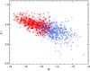 |
Fig. 17 Distribution of the inner (red diamonds) and outer (blue crosses) region samples in the g−r vs. Mr color–magnitude diagram. |
4.5. Ionizing and photometric masses
The estimation of ionizing and total stellar masses provides more information about the average evolutionary stages for both region samples. Considering the number of ionizing photons for each H ii region calculated in Sect. 4.1, we estimated the ionizing cluster masses of the regions using the total number of ionizing photons per unit mass provided by the PopStar models (Mollá et al. 2009) for a zero-age main sequence with Salpeter initial mass function with lower and upper mass limits of 1 and 100 M⊙ and Z = 0.008. For the inner regions sample we obtain a range of values between 2.43 × 10³−7.66 × 10⁶M⊙, whereas a range of 4.66 × 10²−7.36 × 10⁵M⊙ is obtained for the outer regions sample. In principle, these values are lower limits of the ionizing masses, as we are considering an unevolved stellar population with no photon escape and no dust absorption. The maximum effect of the stellar population evolution can be estimated considering the total number of ionizing photons per unit mass given by the PopStar models with the same IMF and metallicity for a population of 5.2 Myr, as PopStar models consider that clusters older than this age do not produce a visible emission-line ionizing spectrum (Martín-Manjón et al. 2010). With those conditions the ionizing mass ranges obtained are one order of magnitude larger than those obtained for the zero-age main sequence population.
One can also estimate photometric masses for the observed regions from the V magnitudes and B−V colors obtained as explained in Sect. 4.4, applying the mass-to-light relation described in Bell & de Jong (2001) for a scaled Salpeter IMF and a formation epoch model with bursts. Figure 18 shows the relation between the obtained photometric mass values and the ratio between ionizing and photometric masses for both region samples. We observe that inner regions have photometric masses two orders of magnitude bigger than outer regions on average. This is to be expected, due to the higher preponderance of underlying stellar populations from the galaxy bulge in the most internal circumnuclear regions. But again we could also think about a possible selection bias, causing that only the biggest inner regions were detected, but the study of the regions angular areas in Sect. 4.1 already showed that the influence of this bias is small, and therefore there is an intrinsic difference between inner and outer photometric masses. Interestingly enough, the ratios between ionizing masses and photometric masses are similar for inner and outer regions, with the outer regions’ ratio values being slightly higher.
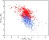 |
Fig. 18 Relation between the photometric mass values and the ratio between ionizing and photometric masses for the inner (red diamonds) and outer (blue crosses) regions samples. |
5. Summary and conclusions
We have analyzed and compared a sample of 725 inner H ii regions, defined following the criterium by Álvarez-Álvarez et al. (2015), and a sample of 671 outer H ii regions, located further than 2 Reff from their corresponding galactic center. The H ii regions were detected and extracted applying the HIIexplorer procedure (Sánchez et al. 2012b; Rosales-Ortega et al. 2012) to the observations of a sample of 263 isolated spiral galaxies, part of the CALIFA survey (Sánchez et al. 2012a).
Different trends and values of the main physical properties of H ii regions are observed in the comparison between inner and outer regions samples. Inner regions show lower hydrogen line equivalent width values, higher extinction and higher luminosities and number of ionizing photons, as well as larger values of [N ii] λ6583/Hα and [O ii] λ3727/[O iii] λ5007 line ratios, related to higher oxygen abundances and smaller ionization parameters respectively. According to these facts we conclude that inner regions have more evolved stellar populations and are in a later evolution state with respect to the outer regions. The distribution of both region samples across several diagnostic diagrams confirm this conclusion.
We have calculated magnitudes and colors from the regions extracted spectra, observing that inner regions are redder and have higher luminosities, as expected. We have also estimated the photometric stellar masses and the ionizing stellar masses of the regions, obtaining higher masses for the inner regions and slightly higher Mion/Mphot values for the outer regions.
This characterization of observational properties of two homogeneous and coherent inner and outer regions samples confirm and expand previous results about intrinsic differences depending on the location of the regions and the influence of the environment, related to different evolution stages and therefore providing information about the formation and evolution processes of the galaxies. These different aspects will be further explored in the second paper of this series by combining both stellar population and photoionization models.
Acknowledgments
We acknowledge financial support for the ESTALLIDOS collaboration by the Spanish Ministerio de Economía y Competitividad (MINECO) under grant AYA2013-47742-C4-3-P. We acknowledge financial support from the Marie Curie FP7-PEOPLE-2013-IRSES scheme, under the SELGIFS collaboration (Study of Emission-Line Galaxies with Integral-Field Spectroscopy). M.R.B. acknowledges financial support by the Spanish Ministerio de Economía y Competitividad under the FPI fellowships program.
References
- Alloin, D., Collin-Souffrin, S., Joly, M., & Vigroux, L. 1979, A&A, 78, 200 [Google Scholar]
- Álvarez-Álvarez, M., Díaz, A. I., Terlevich, E., & Terlevich, R. 2015, MNRAS, 451, 3173 [NASA ADS] [CrossRef] [Google Scholar]
- Baldwin, J. A., Phillips, M. M., & Terlevich, R. 1981, PASP, 93, 5 [NASA ADS] [CrossRef] [EDP Sciences] [Google Scholar]
- Baldwin, J. A., Ferland, G. J., Martin, P. G., et al. 1991, ApJ, 374, 580 [NASA ADS] [CrossRef] [Google Scholar]
- Bell, E. F., & de Jong, R. S. 2001, ApJ, 550, 212 [NASA ADS] [CrossRef] [Google Scholar]
- Bresolin, F., & Kennicutt, R. C. 2015, MNRAS, 454, 3664 [NASA ADS] [CrossRef] [Google Scholar]
- Bresolin, F., Garnett, D. R., & Kennicutt, R. C., Jr. 2004, ApJ, 615, 228 [NASA ADS] [CrossRef] [Google Scholar]
- Cardelli, J. A., Clayton, G. C., & Mathis, J. S. 1989, ApJ, 345, 245 [NASA ADS] [CrossRef] [Google Scholar]
- Cid Fernandes, R., Stasińska, G., Schlickmann, M. S., et al. 2010, MNRAS, 403, 1036 [NASA ADS] [CrossRef] [Google Scholar]
- Cid Fernandes, R., Pérez, E., García Benito, R., et al. 2013, A&A, 557, A86 [NASA ADS] [CrossRef] [EDP Sciences] [Google Scholar]
- Cid Fernandes, R., González Delgado, R. M., García Benito, R., et al. 2014, A&A, 561, A130 [NASA ADS] [CrossRef] [EDP Sciences] [Google Scholar]
- Contini, T., Considere, S., & Davoust, E. 1998, A&AS, 130, 285 [NASA ADS] [CrossRef] [EDP Sciences] [Google Scholar]
- de Vaucouleurs, G., de Vaucouleurs, A., Corwin, H. G., Jr., et al. 1991, Third Reference Catalogue of Bright Galaxies (Springer) [Google Scholar]
- Díaz, Á. I. 1989, in Evolutionary Phenomena in Galaxies (Cambridge University Press), 377 [Google Scholar]
- Díaz, A. I., Castellanos, M., Terlevich, E., & Luisa García-Vargas, M. 2000, MNRAS, 318, 462 [NASA ADS] [CrossRef] [Google Scholar]
- Díaz, Á. I., Terlevich, E., Castellanos, M., & Hägele, G. F. 2007, MNRAS, 382, 251 [NASA ADS] [CrossRef] [Google Scholar]
- Eastman, R. G., Schmidt, B. P., & Kirshner, R. 1996, ApJ, 466, 911 [NASA ADS] [CrossRef] [Google Scholar]
- Falcón-Barroso, J., Sánchez-Blázquez, P., Vazdekis, A., et al. 2011, A&A, 532, A95 [NASA ADS] [CrossRef] [EDP Sciences] [Google Scholar]
- Ferguson, A. M. N., Gallagher, J. S., & Wyse, R. F. G. 1998, AJ, 116, 673 [NASA ADS] [CrossRef] [Google Scholar]
- García-Benito, R., Zibetti, S., Sánchez, S. F., et al. 2015, A&A, 576, A135 [NASA ADS] [CrossRef] [EDP Sciences] [Google Scholar]
- García-Vargas, M. L., Mollá, M., & Martín-Manjón, M. L. 2013, MNRAS, 432, 2746 [NASA ADS] [CrossRef] [Google Scholar]
- Girardi, L., Bertelli, G., Bressan, A., et al. 2002, A&A, 391, 195 [NASA ADS] [CrossRef] [EDP Sciences] [Google Scholar]
- González Delgado, R. M., & Pérez, E. 1997, ApJS, 108, 199 [NASA ADS] [CrossRef] [Google Scholar]
- Gonzalez-Delgado, R. M., Perez, E., Diaz, A. I., et al. 1995, ApJ, 439, 604 [NASA ADS] [CrossRef] [Google Scholar]
- Haynes, M. P., van Zee, L., Hogg, D. E., Roberts, M. S., & Maddalena, R. J. 1998, AJ, 115, 62 [NASA ADS] [CrossRef] [Google Scholar]
- Heidmann, J., Heidmann, N., & de Vaucouleurs, G. 1972, MmRAS, 75, 85 [Google Scholar]
- Hendry, M. A., Smartt, S. J., Maund, J. R., et al. 2005, MNRAS, 359, 906 [NASA ADS] [CrossRef] [Google Scholar]
- Henry, R. B. C. 1993, MNRAS, 261, 306 [NASA ADS] [CrossRef] [Google Scholar]
- Holmberg, E. 1958, Meddelanden fran Lunds Astronomiska Observatorium Serie II, 136, 1 [NASA ADS] [Google Scholar]
- Hoyos, C., & Díaz, A. I. 2006, MNRAS, 365, 454 [NASA ADS] [CrossRef] [Google Scholar]
- Husemann, B., Jahnke, K., Sánchez, S. F., et al. 2013, A&A, 549, A87 [NASA ADS] [CrossRef] [EDP Sciences] [Google Scholar]
- Kauffmann, G., Heckman, T. M., Tremonti, C., et al. 2003, MNRAS, 346, 1055 [Google Scholar]
- Kehrig, C., Monreal-Ibero, A., Papaderos, P., et al. 2012, A&A, 540, A11 [NASA ADS] [CrossRef] [EDP Sciences] [Google Scholar]
- Kelz, A., & Roth, M. M. 2006, New A Rev., 50, 355 [Google Scholar]
- Kelz, A., Verheijen, M. A. W., Roth, M. M., et al. 2006, PASP, 118, 129 [NASA ADS] [CrossRef] [Google Scholar]
- Kennicutt, R. C., Jr., Keel, W. C., & Blaha, C. A. 1989, AJ, 97, 1022 [NASA ADS] [CrossRef] [Google Scholar]
- Kewley, L. J., Dopita, M. A., Sutherland, R. S., Heisler, C. A., & Trevena, J. 2001, ApJ, 556, 121 [Google Scholar]
- Lejeune, T., Cuisinier, F., & Buser, R. 1997, A&AS, 125, 229 [NASA ADS] [CrossRef] [EDP Sciences] [Google Scholar]
- Leonard, D. C., Filippenko, A. V., Li, W., et al. 2002, AJ, 124, 2490 [NASA ADS] [CrossRef] [Google Scholar]
- Lopez, L. A., Krumholz, M. R., Bolatto, A. D., Prochaska, J. X., & Ramirez-Ruiz, E. 2011, ApJ, 731, 91 [NASA ADS] [CrossRef] [Google Scholar]
- López-Hernández, J., Terlevich, E., Terlevich, R., et al. 2013, MNRAS, 430, 472 [NASA ADS] [CrossRef] [Google Scholar]
- Lu, N. Y., Hoffman, G. L., Groff, T., Roos, T., & Lamphier, C. 1993, ApJS, 88, 383 [NASA ADS] [CrossRef] [Google Scholar]
- Makarov, D., Prugniel, P., Terekhova, N., Courtois, H., & Vauglin, I. 2014, A&A, 570, A13 [Google Scholar]
- Marino, R. A., Gil de Paz, A., Castillo-Morales, A., et al. 2012, ApJ, 754, 61 [NASA ADS] [CrossRef] [Google Scholar]
- Marino, R. A., Gil de Paz, A., Sánchez, S. F., et al. 2016, A&A, 585, A47 [NASA ADS] [CrossRef] [EDP Sciences] [Google Scholar]
- Mármol-Queraltó, E., Sánchez, S. F., Marino, R. A., et al. 2011, A&A, 534, A8 [NASA ADS] [CrossRef] [EDP Sciences] [Google Scholar]
- Martín-Manjón, M. L., García-Vargas, M. L., Mollá, M., & Díaz, A. I. 2010, MNRAS, 403, 2012 [NASA ADS] [CrossRef] [Google Scholar]
- Mas-Hesse, J. M., & Kunth, D. 1991, A&AS, 88, 399 [NASA ADS] [Google Scholar]
- Mast, D., Rosales-Ortega, F. F., Sánchez, S. F., et al. 2014, A&A, 561, A129 [NASA ADS] [CrossRef] [EDP Sciences] [Google Scholar]
- Mathis, J. S. 1986, PASP, 98, 995 [NASA ADS] [CrossRef] [Google Scholar]
- Mollá, M., García-Vargas, M. L., & Bressan, A. 2009, MNRAS, 398, 451 [NASA ADS] [CrossRef] [Google Scholar]
- Oey, M. S., & Kennicutt, R. C., Jr. 1993, ApJ, 411, 137 [NASA ADS] [CrossRef] [Google Scholar]
- Oey, M. S., Parker, J. S., Mikles, V. J., & Zhang, X. 2003, AJ, 126, 2317 [NASA ADS] [CrossRef] [Google Scholar]
- Opik, E. 1923, The Observatory, 46, 51 [NASA ADS] [Google Scholar]
- Osterbrock, D. E., & Ferland, G. J. 2006, Astrophysics of gaseous nebulae and active galactic nuclei, 2edn. eds. D. E. Osterbrock, & G. J. Ferland (Sausalito, CA: University Science Books), 2006 [Google Scholar]
- Pérez-Montero, E., & Contini, T. 2009, MNRAS, 398, 949 [NASA ADS] [CrossRef] [Google Scholar]
- Pérez-Montero, E., & Díaz, A. I. 2005, MNRAS, 361, 1063 [NASA ADS] [CrossRef] [Google Scholar]
- Perinotto, M. 1983, NATO Advanced Science Institutes (ASI) Series C, 110, 205 [Google Scholar]
- Rosales-Ortega, F. F. 2009, Ph.D. Thesis, University of Cambridge [Google Scholar]
- Rosales-Ortega, F. F., Kennicutt, R. C., Sánchez, S. F., et al. 2010, MNRAS, 405, 735 [NASA ADS] [Google Scholar]
- Rosales-Ortega, F. F., Díaz, A. I., Kennicutt, R. C., & Sánchez, S. F. 2011, MNRAS, 415, 2439 [NASA ADS] [CrossRef] [Google Scholar]
- Rosales-Ortega, F. F., Sánchez, S. F., Iglesias-Páramo, J., et al. 2012, ApJ, 756, L31 [NASA ADS] [CrossRef] [Google Scholar]
- Rosolowsky, E., Simon, J. D., 2008, ApJ, 675, 1213 [NASA ADS] [CrossRef] [Google Scholar]
- Roth, M. M., Kelz, A., Fechner, T., et al. 2005, PASP, 117, 620 [NASA ADS] [CrossRef] [Google Scholar]
- Saha, A., Thim, F., Tammann, G. A., Reindl, B., & Sandage, A. 2006, ApJS, 165, 108 [NASA ADS] [CrossRef] [Google Scholar]
- Sánchez, S. F., García-Lorenzo, B., Jahnke, K., et al. 2006, Astron. Nachr., 327, 167 [NASA ADS] [CrossRef] [Google Scholar]
- Sánchez, S. F., Rosales-Ortega, F. F., Kennicutt, R. C., et al. 2011, MNRAS, 410, 313 [NASA ADS] [CrossRef] [Google Scholar]
- Sánchez, S. F., Kennicutt, R. C., Gil de Paz, A., et al. 2012a, A&A, 538, A8 [NASA ADS] [CrossRef] [EDP Sciences] [Google Scholar]
- Sánchez, S. F., Rosales-Ortega, F. F., Marino, R. A., et al. 2012b, A&A, 546, A2 [NASA ADS] [CrossRef] [EDP Sciences] [Google Scholar]
- Sánchez, S. F., Rosales-Ortega, F. F., Iglesias-Páramo, J., et al. 2014, A&A, 563, A49 [NASA ADS] [CrossRef] [EDP Sciences] [Google Scholar]
- Sánchez, S. F., Pérez, E., Rosales-Ortega, F. F., et al. 2015, A&A, 574, A47 [NASA ADS] [CrossRef] [EDP Sciences] [Google Scholar]
- Sánchez, S. F., García-Benito, R., Zibetti, S., et al. 2016a, A&A, 594, A36 [NASA ADS] [CrossRef] [EDP Sciences] [Google Scholar]
- Sánchez, S. F., Pérez, E., Sánchez-Blázquez, P., et al. 2016b, Rev. Mexicana Astron. Astrofis., 52, 21 [Google Scholar]
- Sánchez, S. F., Pérez, E., Sánchez-Blázquez, P., et al. 2016c, Rev. Mexicana Astron. Astrofis., 52, 171 [Google Scholar]
- Sánchez-Menguiano, L., Sánchez, S. F., Kawata, D., et al. 2016, ApJ, 830, L40 [NASA ADS] [CrossRef] [Google Scholar]
- Schawinski, K., Urry, C. M., Simmons, B. D., et al. 2014, MNRAS, 440, 889 [NASA ADS] [CrossRef] [Google Scholar]
- Springob, C. M., Haynes, M. P., Giovanelli, R., & Kent, B. R. 2005, ApJS, 160, 149 [Google Scholar]
- van Zee, L., Salzer, J. J., Haynes, M. P., O’Donoghue, A. A., & Balonek, T. J. 1998, AJ, 116, 2805 [NASA ADS] [CrossRef] [Google Scholar]
- Vazdekis, A., Sánchez-Blázquez, P., Falcón-Barroso, J., et al. 2010, MNRAS, 404, 1639 [NASA ADS] [Google Scholar]
- Verheijen, M. A. W., Bershady, M. A., Andersen, D. R., et al. 2004, Astron. Nachr., 325, 151 [NASA ADS] [CrossRef] [Google Scholar]
- Véron-Cetty, M.-P., & Véron, P. 2006, A&A, 455, 773 [NASA ADS] [CrossRef] [EDP Sciences] [Google Scholar]
- Walcher, C. J., Wisotzki, L., Bekeraité, S., et al. 2014, A&A, 569, A1 [NASA ADS] [CrossRef] [EDP Sciences] [Google Scholar]
- Werk, J. K., Putman, M. E., Meurer, G. R., et al. 2010, AJ, 139, 279 [NASA ADS] [CrossRef] [Google Scholar]
- Willett, K. W., Lintott, C. J., Bamford, S. P., et al. 2013, MNRAS, 435, 2835 [NASA ADS] [CrossRef] [Google Scholar]
- York, D. G., Adelman, J., Anderson, J. E., Jr., et al. 2000, AJ, 120, 1579 [CrossRef] [Google Scholar]
All Tables
Physical properties of part of the CALIFA galaxies involved in this work, as described in the text.
Physical properties of the PINGS galaxies involved in this work, obtained from the following sources.
Physical properties of outer regions located further than 6 Reff from their galaxy center.
All Figures
|
Fig. 1 Redshifts values (left) and of distance values in Mpc (right). Both histograms correspond to the galaxy sample of this work. |
| In the text | |
|
Fig. 2 Distribution of morphological types for the galaxy sample of this work. |
| In the text | |
|
Fig. 3 Inclination values for this work galaxy sample, calculated from the observed axis ratios. Values of all galaxies are represented in dark blue, and overplotted in light blue are the values of the galaxies with Mr> −18.6. |
| In the text | |
|
Fig. 4 Effective radius values (kpc) of this work galaxy sample. |
| In the text | |
|
Fig. 5 Distribution of this work galaxy sample in the g−r vs. Mr color–magnitude diagram. |
| In the text | |
|
Fig. 6 Some of the inner regions extracted spectra, before the subtraction of the stellar continuum. Galaxy name, ID of the region in the galaxy and distance to the center are shown in the titles. Flux is expressed in units of 10-16 erg s-1 cm-2. |
| In the text | |
|
Fig. 7 Some of the outer regions extracted spectra, before the subtraction of the stellar continuum. Galaxy name, ID of the region in the galaxy and distance to the center are shown in the titles. Flux is expressed in units of 10-16 erg s-1 cm-2. |
| In the text | |
|
Fig. 8 From top to bottom and left to right: equivalent width of Hα, dust attenuation, Hα luminosity and of the [N ii] λ6583/Hα, [O ii] λ3727/[O iii] λ5007, and [S ii] λ6717/[S ii] λ6731 emission-line ratios for the inner (red diagonally-hatched diagram) and outer (blue horizontally-hatched diagram) region samples. |
| In the text | |
|
Fig. 9 Left column: EW(Hα) and AV histograms from the inner H ii regions sample as a function of their galaxies morphological types. Regions with Sa, Sab and Sb type galaxies are colored in dark red, those with Sbc, Sc and Scd type galaxies in orange and those with Sd, Sdm and Sm type galaxies are colored in gold. EW(Hα) is expressed in units of Å and AV in magnitudes. Right column: histograms with the same parameters as those from the outer H ii regions sample. Regions with Sa, Sab and Sb type galaxies are colored in dark blue, those with Sbc, Sc and Scd type galaxies in blue and those with Sd, Sdm and Sm type galaxies are colored in light blue. |
| In the text | |
|
Fig. 10 Number of ionizing photons for the inner (red diagonally-hatched diagram) and outer (blue horizontally-hatched diagram) region samples. |
| In the text | |
|
Fig. 11 Angular area in arcsec2 for the inner (red diagonally-hatched diagram) and outer (blue horizontally-hatched diagram) region samples. |
| In the text | |
|
Fig. 12 Left: diagnostic diagram of the CALIFA inner region sample (red circles). Data from PINGS inner region sample (black diamonds), from CNSFR (green asterisks) studied by Díaz et al. (2007) and from central region (dark green triangle) of M33 studied by López-Hernández et al. (2013) are also included for comparison. Right: diagnostic diagram of the CALIFA outer region sample (blue circles). Different shades correspond to different bins of distance to the center of the galaxy, as indicated. Point from the IC 132 H ii region (orange square) of M33 studied by López-Hernández et al. (2013) is included for comparison. Overplotted as black lines in both diagrams are empirically and theoretically derived separations between LINERs/Seyferts and H ii regions. |
| In the text | |
|
Fig. 13 Relation between [O ii] λ3727/[O iii] λ5007 emission-line ratio and the O3N2 index for the CALIFA inner (red diamonds) and outer (blue crosses) regions samples. Data from PINGS inner region sample (black stars), from CNSFR (dark green asterisks) studied by Díaz et al. (2007) and from central region (light green triangle) and IC 132 H ii region (orange square) of M33 studied by López-Hernández et al. (2013) are also included for comparison. |
| In the text | |
|
Fig. 14 Relation between [N ii] λ6583/[O ii] λ3727 emission-line ratio and the O3N2 index for the CALIFA inner (red diamonds) and outer (blue crosses) region samples. Data from PINGS inner region sample (black stars), from CNSFR (dark green asterisks) studied by Díaz et al. (2007) and from central region (light green triangle) and IC 132 H ii region of M33 (orange square) studied by López-Hernández et al. (2013) are also included for comparison. |
| In the text | |
|
Fig. 15 Relation between EW(Hβ) and [O ii] λ3727/[O iii] λ5007 emission-line ratio for the inner (red diamonds) and outer (blue crosses) regions samples. Overplotted as a dashed black line is the relation given by Hoyos & Díaz (2006), explained in the text. |
| In the text | |
|
Fig. 16 Spectra from two of the ten H ii regions located further than 6 Reff from their galaxy center, before the subtraction of the stellar continuum. Galaxy name, ID of the region in the galaxy and distance to the center are shown in the titles. Flux is expressed in units of 10-16 erg s-1 cm-2. |
| In the text | |
|
Fig. 17 Distribution of the inner (red diamonds) and outer (blue crosses) region samples in the g−r vs. Mr color–magnitude diagram. |
| In the text | |
|
Fig. 18 Relation between the photometric mass values and the ratio between ionizing and photometric masses for the inner (red diamonds) and outer (blue crosses) regions samples. |
| In the text | |
Current usage metrics show cumulative count of Article Views (full-text article views including HTML views, PDF and ePub downloads, according to the available data) and Abstracts Views on Vision4Press platform.
Data correspond to usage on the plateform after 2015. The current usage metrics is available 48-96 hours after online publication and is updated daily on week days.
Initial download of the metrics may take a while.