| Issue |
A&A
Volume 609, January 2018
|
|
|---|---|---|
| Article Number | A29 | |
| Number of page(s) | 10 | |
| Section | Stellar structure and evolution | |
| DOI | https://doi.org/10.1051/0004-6361/201731427 | |
| Published online | 22 December 2017 | |
Sensitivity of the s-process nucleosynthesis in AGB stars to the overshoot model
Institut d’Astronomie et d’Astrophysique, Université Libre de Bruxelles (ULB), CP 226, 1050 Brussels, Belgium
e-mail: This email address is being protected from spambots. You need JavaScript enabled to view it.
Received: 23 June 2017
Accepted: 22 August 2017
Abstract
Context. S-process elements are observed at the surface of low- and intermediate-mass stars. These observations can be explained empirically by the so-called partial mixing of protons scenario leading to the incomplete operation of the CN cycle and a significant primary production of the 13C neutron source. This scenario has been successful in qualitatively explaining the s-process enrichment in AGB stars. Even so, it remains difficult to describe both physically and numerically the mixing mechanisms taking place at the time of the third dredged-up between the convective envelope and the underlying C-rich radiative layer
Aims. We aim to present new calculations of the s-process nucleosynthesis in AGB stars testing two different numerical implementations of chemical transport. These are based on a diffusion equation which depends on the second derivative of the composition and on a numerical algorithm where the transport of species depends linearly on the chemical gradient.
Methods. The s-process nucleosynthesis resulting from these different mixing schemes is calculated with our stellar evolution code STAREVOL which has been upgraded to include an extended s-process network of 411 nuclei. Our investigation focuses on a fiducial 2 M⊙, [Fe/H] = −0.5 model star, but also includes four additional stars of different masses and metallicities.
Results. We show that for the same set of parameters, the linear mixing approach produces a much larger 13C-pocket and consequently a substantially higher surface s-process enrichment compared to the diffusive prescription. Within the diffusive model, a quite extreme choice of parameters is required to account for surface s-process enrichment of 1–2 dex. These extreme conditions can not, however, be excluded at this stage.
Conclusions. Both the diffusive and linear prescriptions of the overshoot mixing are suited to describe the s-process nucleosynthesis in AGB stars provided the profile of the diffusion coefficient below the convective envelope is carefully chosen. Both schemes give rise to relatively similar distributions of s-process elements, but depending on the parameters adopted, some differences may be obtained. These differences are in the element distribution, and most of all in the level of surface enrichment.
Key words: nuclear reactions, nucleosynthesis, abundances / stars: AGB and post-AGB
© ESO, 2017
1. Introduction
The determination of the surface composition of evolved stars provides important clues to the evolution of their internal structure and their role in the cosmic cycle. In that respect, asymptotic giant branch (AGB) stars form an important class of objects for several reasons. They correspond to the late evolutionary phase of stars with masses between about 1 and 8 M⊙; they exhibit peculiar chemical patterns at their surface as compared to other red giant stars; and many of them are characterized by strong mass loss (up to 10-4M⊙ yr-1) that ejects the surface material into the interstellar medium, contributing thereby to the galactic chemical evolution.
The abundance peculiarities observed at the surface of AGB stars are the consequence of (i) H-burning at the base of the convective envelope during the so-called hot bottom burning that can lead to a temporary production of  and affects the CNO isotopes,
  or
or  and (ii) the action of the third dredge-up (denoted hereafter 3DUP) that allows elements synthesized in the He-burning layers to reach the surface. The signatures of the 3DUP are multiple and can explain, for example, the formation of carbon stars, and the surface enrichment in
  , Mg isotopes or heavy elements such as Ba or Pb by the so-called slow neutron capture process (for a recent review, see Karakas & Lattanzio 2014). The
  reaction is currently believed to be the major neutron source in low-mass AGB stars leading to the production of s-process elements (Busso et al. 1999). In more massive AGB stars, neutrons can also be released at the bottom of the thermal pulse by the
  reaction. This production requires high temperatures (T ≳ 3.2 × 10⁸ K) achieved in stars with M ≳ 3−4M⊙, depending on the metallicity. The canonical scenario to produce fresh
  is to invoke the mixing of protons from the envelope into the
  -rich layers during a 3DUP event (e.g., Iben & Renzini 1982), followed by the incomplete operation of the CN cycle. The region over which protons are transported is referred to as the partial mixing (PM) zone. Unfortunately, AGB models are still subject to large uncertainties concerning the consistent prediction of both the 3DUP and transport processes. In particular, the 3DUP and PM properties are sensitive to the stellar characteristics (such as stellar mass, metallicity or mass loss rate) and strongly depend on the numerical and physical treatment of the convective boundaries and more specifically on the prescriptions used to account for extra-mixing at the base of the envelope. These additional transport processes are generally attributed to convective overshooting (Herwig et al. 1997), rotationally induced mixing (Herwig et al. 2003; Siess et al. 2004; Piersanti et al. 2013), gravity waves (Denissenkov & Tout 2003) or mixing driven by magnetic buoyancy (Nucci & Busso 2014) but remain parametric and poorly constrained. Recent attempts to perform two- and three-dimensional hydrodynamical simulation of the He shell convective zone below the AGB envelope (Herwig et al. 2006, 2014; Stancliffe et al. 2011) provide some hints on the nature of the mixing but the resolution and short time scales of the simulations still limit their predictive power.
This paper investigates the impact on the s-process nucleosynthesis of the numerical treatment of overshoot mixing at the base of the convective envelope in AGB star. In Sect. 2, we describe the different prescriptions adopted for the implementation of the chemical transport and the nuclear ingredients for the s-process reaction network included in our stellar evolution code STAREVOL. The nucleosynthesis of the heavy elements is analyzed in details for a fiducial 2 M⊙[Fe/H] = −0.5 model star up to the end of the AGB phase. In Sect. 3, we study the abundance redistribution of heavy elements (A ≳ 40) due to the neutron captures taking place during the core He-burning phase. In Sect. 4, we pay special attention to the s-process taking place during the AGB phase with a detailed study of its sensitivity with respect to different overshoot models and different choices of their parameters. We also discuss the final surface abundances for stars of different masses and metallicities in Sect. 5. We finally draw our conclusions in Sect. 6.
2. Mixing and nucleosynthesis modeling
The present calculations are based on the stellar evolution code STAREVOL, the description of which can be found in Siess et al. (2000), Siess (2006) and references therein. In our computations, we have used the standard mixing length theory (MLT) with α = 1.75 and take into account the change in opacity due to the formation of molecules when the star becomes carbon rich, as prescribed by Marigo (2002). The reference solar composition is given by Asplund et al. (2009) which corresponds to a metallicity Z = 0.0134. For the mass loss rate, we used the Reimers (1975) prescription with ηR = 0.4 from the main sequence up to the beginning of the AGB and then switched to the Vassiliadis & Wood (1993) rate. The following sections describe in more detail our extended treatments of chemical transport and nuclear burning that have now been consistently included in STAREVOL. We stress that in the present study, we have not considered extra-mixing at the boundaries of the thermal pulse, but only at the base of the convective envelope.
2.1. An empirical description of the convective overshoot
The temperature gradient in the convective regions is usually computed by means of the MLT where the radial fluid velocity (vconv) depends on the local thermodynamical properties. From this velocity, a diffusion coefficient is defined:  (1)where Λ = αHp is the mixing length, α the MLT parameter and Hp the pressure scale height. This local time-independent theory predicts that at the convective boundary the acceleration of the convective bubbles (but not its velocity) vanishes. However, pushed by their inertia, nothing can prevent the convective cells to overshoot beyond the Schwarzschild limit. This extension of the mixing is usually referred to as overshooting.
In stellar evolution calculations, essentially two standard prescriptions have been proposed to describe convective overshooting. The first and oldest one simply assumes that the convective zone extends over of fraction  beyond the Schwarzschild limits, where
  is the pressure scale height at the convective boundary. The value of d was constrained by fitting the width of massive main sequence stars (e.g., Maeder & Meynet 1987) and varies between ≈0.1−0.25. The other alternative was proposed by Herwig et al. (1997; see also Herwig 2000) based on the two-dimensional hydrodynamical simulations of Freytag et al. (1996) and assumes a diffusion coefficient in the overshoot region of the form
  (2)where Dcb is the value of the diffusion coefficient at the base of the convective envelope (as defined by the Schwarzschild criterion), z is the distance from the formal convective boundary and fover a free parameter describing the efficiency of the diffusive mixing. In a more recent paper, Battino et al. (2016) upgraded this prescription by implementing a double exponential where a second flatter exponential term takes over when the diffusion coefficient has fallen below a threshold value D2 ≈ 105 cm2/ s. This second term was fitted on a 3 M⊙ model to account for the mixing induced by gravity waves. Their formulation corresponds to
 ![Mathematical equation: \begin{eqnarray} D_{\over}= \begin{cases} \displaystyle D_{\rm cb} \exp{\left( \frac{-2z}{f_{1} H_{\rm p}^{\rm cb}}\right)} \ \ \ \ \ \ \ \ \text{if }z<z_2 \\[6mm] \displaystyle D_{2} \exp{\left( \frac{-2(z-z_2)}{f_{2} H_{\rm p}^{\rm cb}}\right)} \ \ \ \text{if }z>z_2, \\ \end{cases} \label{eq_Herwig2} \end{eqnarray}](/articles/aa/full_html/2018/01/aa31427-17/aa31427-17-eq39.png) (3)where the switch between the two regimes occurs at the depth z2, determined by imposing that
(3)where the switch between the two regimes occurs at the depth z2, determined by imposing that  (4)In this prescription, z is the distance from the convective boundary and the parameters are f1,f2 and D2. During the AGB phase, Battino et al. (2016) use the default values of f1 = 0.014, D2 = 1011 cm2/ s and f2 = 0.25 at the bottom of the convective envelope.
Essentially, two different approaches can be found in the literature regarding the numerical implementation of the chemical transport. The diffusive mixing scheme (referred to as DM) describes the transport of the nuclear species by a diffusion equation ![Mathematical equation: \begin{equation} \frac{\partial X}{\partial t}= \frac{\partial}{\partial m_r} \left[\,(4 \pi r^2 \rho)^2\,D\ \frac{\partial X}{\partial m_r}\right] , \label{eq_dif} \end{equation}](/articles/aa/full_html/2018/01/aa31427-17/aa31427-17-eq47.png) (5)where D = Dconv + Dover is the sum of the convective and overshoot diffusion coefficients, respectively. However, a diffusive approach of this process may not be very realistic as convection is in essence the advection of convective bubbles.
(5)where D = Dconv + Dover is the sum of the convective and overshoot diffusion coefficients, respectively. However, a diffusive approach of this process may not be very realistic as convection is in essence the advection of convective bubbles.
An alternative algorithm was devised by Sparks & Endal (1980) and later improved by Chieffi et al. (2001) and Straniero et al. (2006) where mixing is now described by a linear equation coupling the mixing between neighboring layers moving at a velocity v over a time step Δt. This formulation, which we refer to as linear mixing (LM), is given by  (6)In this expression the summation runs overs the whole zone affected by mixing and the superscript 0 refers to abundances prior to the mixing. ΔMk is the mass of the layer k and the factor
 ![Mathematical equation: \begin{equation} f_{j,k}= \left\{\begin{array}{ll} \Delta t/\tau_{j,k} & \mathrm{if\ } \Delta t \le \tau_{j,k}, \\[4mm] 1 & \mathrm{if\ } \Delta t > \tau_{j,k}, \end{array}\right. \end{equation}](/articles/aa/full_html/2018/01/aa31427-17/aa31427-17-eq55.png) (7)where the mixing turnover time between mesh points j and k is given by
(7)where the mixing turnover time between mesh points j and k is given by  (8)where Δri = ri + 1−ri is the size of the cell. The velocity vi is set to vconv in the convective layers and below the envelope it decreases exponentially with
  where vcb is the velocity at the base of the convective envelope and β a free parameter. We note that this formulation is equivalent to the expression for Dover given by Eq. (2).
In our computation, the total mass of the mixing zone was calculated as Mmix = ∑ kΔMk × fk with fk = Δt/τk = Δt × vk/ Δrk if Δt<τk, or 1 otherwise. In comparison with the standard expression provided by Straniero et al. (2006) where Mmix = ∑ kΔMk, our formulation presents the advantage of being independent of the limit in the summation, since in the layers where mixing is not present vk and fk = 0.
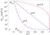 |
Fig. 1 Profile of the overshoot diffusion coefficient Dover as a function of the reduced depth z/z∗ for different values of p and assuming Dcb = 1016 cm2/ s, Dmin = 103 cm2/ s. |
In the present study, we have considered both the DM (Eq. (5)) and LM (Eq. (6)) prescriptions and in each case, the adopted mathematical profile for the overshoot diffusion coefficient reads  (9)where the characteristic length z∗ is given by z∗ = fover × Hp × ln(Dcb)/2, Dmin is the value of the diffusion coefficient at the boundary z = z∗ and p is an additional free parameters defining the slope of the exponential decrease of Dover with respect to z. Some examples of the z-dependence of the overshoot diffusion coefficient are illustrated in Fig. 1. Note that below Dmin we have assumed that Dover drops to zero, in contrast to Straniero et al. (2006) who do not consider a lower limit for vover, hence for Dover. So, with our prescription, the overshoot mixing is only taking place over the radial region defined by 0 ≤ z ≤ z∗. We note that Eq. (9) is just an extension of Eq. (2) from the original formulation of Herwig et al. (1997) which is recovered by setting p = 1 and fover = 0.02 and Dmin = 1 cm2/ s. Similarly, the default parameters used by Straniero et al. (2006) in their simulations correspond to p = 1 and fover = 0.2 and Dmin = 1 cm2/ s. We also point out that for a given value of Dcb, different parameters fover, Dmin and p can lead to similar profiles of Dover for z ≤ z∗. For example for Dcb = 1016 cm2/ s and p = 1, the same profile is obtained using (Dmin = 104 cm2/ s; fover = 0.25) or (Dmin = 1 cm2/ s; fover = 0.2) with the only difference that, in the former case, the diffusion coefficient drops to zero earlier, that is, when Dover reaches 104 cm2/ s.
We also stress that at the time of maximum deepening of the convective envelope during the 3DUP, the size of the CO core is ≈0.3–0.4 R⊙ for our 2 M⊙ model. This number slightly varies with the mixing parameters (which impact the efficiency of the 3DUP) but remains always of the same order of magnitude as  R⊙. As a consequence, using unrealistically large values of fover can lead to proton mixing well below the convective envelope and induce a substantial reduction of the CO core size eventually leading to convergence issues. In practice, values of fover larger than typically 0.1 can hardly be considered in our model star.
In light of the previous remark, we find that using the double exponential prescriptions of Battino et al. (2016) leads to a complete disappearance of the s-process nucleosynthesis. In our stellar models, during the interpulse phase the second exponential term (obtained with the large value of f2 = 0.25) was responsible for the transport of the neutron poison 14N in the region where 13C is burnt. As for rotation (Herwig et al. 2003; Siess et al. 2004), this pollution of the pocket induced by this sustained chemical transport inhibits the production of s-process nuclei. We do not understand why this effect does not show up in the computations of Battino et al. (2016).
2.2. S-process reaction network
A full nuclear reaction network including 411 nuclei between H and Po with some 734 nuclear (n-, p-, and α-captures), weak (electron captures, β-decays) and electromagnetic interactions has been implemented in the STAREVOL code. Nuclear reaction rates were taken from the Nuclear Astrophysics Library of the Brussels University1 (Arnould & Goriely 2006), and include the latest experimental and theoretical cross sections through the interface tool NETGEN (Xu et al. 2013a). In particular, all the charged-particle-induced reaction rates of relevance in the H- and He-burning calculations were taken from the NACRE and NACRE-II evaluations (Angulo et al. 1999; Xu et al. 2013b) as well as STARLIB library (Sallaska et al. 2013). When not available experimentally, the cross sections were calculated within the statistical Hauser-Feshbach model with the TALYS reaction code (Goriely et al. 2008). The TALYS calculations were also used systematically to deduce from the laboratory neutron capture cross sections the stellar rates by allowing for the possible thermalization of low-lying states in the target nuclei. We note that at low temperature, the non-thermalization of the isomeric state of 26Al, 85Kr, 115In, 176Lu and 180Ta is introduced explicitly in the reaction network (Käppeler et al. 1989; Nemeth et al. 1994). The temperature- and density-dependent β-decay and electron capture rates in stellar conditions were taken from Takahashi & Yokoi (1987) with the update of Goriely (1999). The (n,α) reactions and α-decays are also introduced when relevant, in particular for the Bi and Po isotopes.
3. Nucleosynthesis process during core He-burning
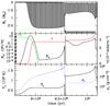 |
Fig. 2 Upper panel: Kippenhahn diagram of our 2 M⊙[Fe/H] = −0.5 during the first dredge-up and core He burning phases; the green and blue dotted lines delineate the region of maximum nuclear energy production by H- and He-burning, respectively. Middle panel: evolution of the central neutron density Nn, central 13C mass fraction (×106) and neutron exposure τ. Lower panel: evolution of the central temperature Tc and density ρc. |
When the star leaves the main sequence and the central temperature reaches ≈5 × 10⁷ K (for a density ρc ≈ 3 × 10⁴ g cm-3), the burning of the CNO by-product 13C via produces a first burst of neutrons (Fig. 2). This occurs during the first dredge-up of our 2 M⊙[Fe/H] = −0.5 model star and leads to a maximum neutron density of Nn = 13 cm-3 and a time-integrated neutron exposure of 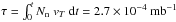 , where vT is the most probable relative neutron-nucleus velocity at the temperature T. The main neutron emission lasts until is depleted at the center and then proceeds at a much lower rate in the contracting shells surrounding the -free core. Eventually helium ignites off-center and after a series of shell flashes, convection reaches the center at an age 9.57 × 10⁸ yr. The temperature in the core reaches 1.2 × 10⁸ K and can trigger the production of a small amount of neutrons by the activation of the
  reaction. The neutron exposure increases up to τ = 3.7 × 10⁻⁴ mb-1 but remains too small to generate an efficient s-process nucleosynthesis. Instead, it is responsible for the re-arrangements of the abundances of specific heavy nuclei. As shown in Fig. 3, elements such as 40K, 108Cd, 128,130Xe, 154Gd, 160Dy, 170Yb or 198Hg can be significantly produced with abundances increased by more than ~0.4 dex with respect to their initial value and others partially destroyed, like 107Ag, 149Sm or 151Eu. At the temperatures encountered in the stellar center during core He burning, we notice that 123Te, 176Lu, 180Ta and 187Os become β-unstable and fully decay (Takahashi & Yokoi 1987). When helium is exhausted in the core, the chemical profiles in the central 0.4–0.5 M⊙ are frozen and the abundances of these heavy nuclei will be part of the future white dwarf. We note that the distributions of overabundances of elements heavier than typically A = 40 show very small differences between our 2 and 3 M⊙ stellar models, almost independently of the metallicity.
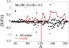 |
Fig. 3 Final overproduction factors [X/Fe] of all stable nuclei with A ≥ 30 (full squares) at the center of our 2 M⊙[Fe/H] = −0.5 model star at the end of core helium burning. The s-only nuclei are shown by red diamonds connected by a solid line. The vertical line depicts the total decay of the s-only nucleus 123Te. |
4. S-process nucleosynthesis during the AGB phase of a 2 M⊙ [Fe/H] = –0.5 model star
Mixing of the nuclear species beyond the convective boundary in the LM and DM models essentially depends on three parameters: Dmin, p and fover. While fover describes the radial extent over which mixing takes place, the other two parameters Dmin and p modify the profile of the diffusion coefficient and thus the distribution of protons in the C-rich region and incidentally the s-process nucleosynthesis. In Sect. 4.1 we first study the proton profiles resulting from the overshooting within the LM and DM models and then analyze the production of s-only nuclei during a given interpulse phase (Sect. 4.2) and in the convective pulse (Sect. 4.3). The surface enrichment resulting from the overshoot mixing since the beginning of the AGB phase is discussed in Sect. 4.4.
4.1. Proton profiles resulting from the treatment of overshoot mixing
To compare the effects of the two mixing schemes, we began our calculations with the same initial model computed without any extra-mixing to avoid any chemical contamination resulting from previous evolution. We recall that we have not considered overshooting at the convective boundaries of the thermal pulse. The initial model is taken at the time when the convective envelope approaches its deepest extent during the 3DUP following the 8th thermal pulse of our 2 M⊙ [Fe/H]=−0.5 model star. We note that the mass coordinate reached by the convective envelope during the 3DUP depends on the mixing scheme.
We show in Fig. 4 the diffusion coefficients and proton mass fractions below the convective envelope obtained with the LM formalism for different values of the parameters Dmin and p. As expected, a more efficient transport resulting for example from a higher value of Dmin or a flatter profile obtained with a lower p leads to a deeper 3DUP. Following Goriely & Mowlavi (2000), we defined the extent of the PM zone ΔMpmz as the mass range over which the hydrogen mass fraction decreases from X(H) = 0.5 (close to its envelope value) to X(H) = 10-5. As shown in Table 1, ΔMpmz varies between ≈6 × 10⁻⁵M⊙ (for p = 1, Dmin = 109 cm2/ s) to almost 7 × 10⁻⁴M⊙ (for p = 1, Dmin = 106 cm2/ s). We also note that with increasing values of Dmin, the H mass fraction remains relatively high in the mixing region and then drops rapidly.
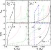 |
Fig. 4 Left panels: proton mass fraction (bottom panel) and diffusion coefficient (top panel) profiles below the convective envelope resulting from the LM scheme with overshoot parameters fover = 0.1, Dmin = 103 cm2/ s and 3 values of p = 1/2, 1, 5. Right panels: same but for fover = 0.1, p = 1 and 4 values of Dmin = 101.9 cm2/ s. The profiles were taken when the convective envelopes reaches its deepest inward extent. For display convenience, the Dmin = 109 profiles have been shifted outward by 0.00085 M⊙. |
Extent in mass (in unit of 10-4M⊙) of the PM zone (ΔMpmz) and s-process region (ΔMspro) for the LM and DM models and the different adopted values of the parameters p and Dmin (in cm2/ s). In all cases, fover = 0.1.
In the DM case (Fig. 5), the extent of the PM zone is systematically smaller by a factor of between three and eight compared with the values obtained with the LM prescription, except in the rather extreme case of Dmin = 109. Although this study has been restricted to a specific interpulse phase, the derived properties (extent of the mixing, H profiles) remain general and weakly dependent on mass or composition as long as the background stellar stratification is not significantly affected (Herwig et al. 2007).
4.2. S-process nucleosynthesis during an interpulse
In this section we analyze the overproduction factors [X/Fe] of the 28 s-only nuclei at the end of the eighth interpulse of our 2 M⊙[Fe/H] = −0.5 model star resulting from the two different mixing schemes (DM and LM). The abundances are determined by averaging the chemical composition over a mass range of 0.01 M⊙ between Mr = 0.595 and 0.605M⊙. We recall that the same initial stellar structure is considered in all cases (the fully consistent stellar evolution sequences are presented in Sects. 4.4 and 5).
The results of our exploration of the mixing parameter space are displayed in Figs. 6 and 7 for the LM and DM schemes, respectively. The first obvious observation is the similarity of the distribution of s-elements between all the models, except may be for the extreme case p = 1, Dmin = 109 cm2/ s. The main difference is the level of overproduction.
During the interpulse phase, the s-process nucleosynthesis is known to take place in a relatively small radiative region where the proton-to-12C ratio ranges between 0.06 and 0.6, although in more metal poor stars with [Fe/H] ≲ −1, layers with ratios as low as 0.002 also contribute (Goriely & Mowlavi 2000). For an He intershell carbon mass fraction X(12C) = 0.2, the neutron production will mainly occur in layers where the proton mass fraction X(H) ≃ 10-3−10-2, while for larger values of X(H) ≃ 10-2−10-1 an efficient production of 19F and 23Na is expected. As discussed in Goriely & Mowlavi (2000), the detailed profile of protons in this region dictates the subsequent s-process nucleosynthesis (see in particular their Fig. 3), so the extent of the PM zone Δpmz as defined in Sect. 4.1 is only a qualitative and approximate indicator of the s-process efficiency. For example, the value of Δpmz picked in Table 1 for the DM scheme is similar between the models Dmin = 1 and Dmin = 109 but the resulting s-process enrichment (Fig. 7) is significantly different. For this reason, we defined a new indicator ΔMspro corresponding to the mass extent where 10-3 ≤ X(H) ≤ 10-2. An inspection of the numbers presented in Table 1 indicates that ΔMpmz and ΔMspro are quite different but strongly correlated. There are, however, two exceptions, one is related to the extreme case Dmin = 109 cm2/ s mentioned previously and the second to the LM cases p = 1/2 and p = 1 where the nucleosynthesis is very similar. Comparing Figs. 6, 7, and Table 1 indicates that the highest overproduction factors are obtained for the largest values of ΔMspro. In the LM case, ΔMspro reaches a maximum of ~3 × 10⁻⁴M⊙ for p = 1/2−1 and Dmin ≈ 103−106 cm2/ s, leading to a significant production of s-process nuclei (Fig. 6). In contrast, in the DM case, ΔMspro never exceeds 3 × 10⁻⁵M⊙, that is, about an order of magnitude lower than in the LM case. As shown in Fig. 7, the overall overproduction factors are indeed a factor of between five and ten lower than in the LM model. This significant enrichment in s-process elements by the LM scheme was also reported by Cristallo et al. (2009).
 |
Fig. 6 Overabundance distributions [X/Fe] for the 28 s-only nuclei inside a region of 0.01 M⊙ around Mr = 0.595−0.605M⊙ at the end of the 8th interpulse of our 2 M⊙[Fe/H] = −0.5 model star. The results are shown for different LM conditions, i.e. different values of p (upper panel) or Dmin (in cm2/s; lower panel); in all cases, fover = 0.1 is assumed. |
4.3. Convective nucleosynthesis in the thermal pulse
The distribution of s-elements resulting from the radiative interpulse nucleosynthesis, as described in Sect. 4.2, may still be affected by the second neutron irradiation taking place in the pulse-driven convective region, at least if the temperature Tp at its base is high enough to activate the reaction. Tp depends on the core mass and is known to increase with increasing pulse number, stellar mass or decreasing metallicities and ranges from 1.5 × 10⁸ K to above 3.5 × 10⁸ K. In our 2 M⊙[Fe/H] = −0.5 model star, Tp reaches 3 × 10⁸ K in the last thermal pulses, so only few neutrons are produced. As seen in Fig. 8, the impact of the convective pulse nucleosynthesis on the abundance distribution of s-only nuclei is negligible. However, locally, the abundances of some nuclei, such as 93Nb, 113In, 176Lu or 187Os may be modified through the impact of T-dependent s-process branching during the neutron irradiation (Takahashi & Yokoi 1987). In the mass and metallicity range considered in this study, none of the 13C produced by the PM of protons survives the interpulse phase. Therefore, it remains to be checked if, in low-mass metal-poor stars (M ≲ 1.5M⊙, [Fe/H] ≲ −2), fresh 13C is ingested in the convective pulse, as found in previous studies (Lugaro et al. 2012).
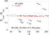 |
Fig. 8 Ratio of the nuclei mass fraction after (Xconv) and before (Xrad) the 9th thermal pulse of our 2 M⊙[Fe/H] = −0.5 model star. Open and filled squares represent stable and s-only nuclei, respectively. |
4.4. Nucleosynthetic yields
In this section, we present the nucleosynthesis yields of a 2 M⊙[Fe/H] = −0.5 model computed with the LM and DM mixing formalisms. For these simulations, the same mixing parameters are used, namely Dmin = 103 cm2/ s, p = 1 and fover = 0.1, and applied since the beginning of the AGB phase. The thermal pulse-AGB evolution is similar in both cases and leads to the occurrence of ten thermal pulses and 8 3DUP. The surface overabundance of s-only nuclei obtained at the end of the computation is presented in Fig. 9. Although the two distributions are relatively similar, the overproduction obtained with the DM is about eight times smaller than with the LM prescription. Again, this has to be ascribed to the smaller mass of the PM zone in the DM formulation. While the LM prescription gives rather satisfactory overproduction factors of the order of 1.5 dex, they do not exceed 0.9 dex in the DM case. The latter would consequently face problems explaining the large surface abundances of some intrinsic s-process-rich C-stars that show for example [Ba/Fe] as high as 1.65 (Zamora et al. 2009).
In the specific DM case, we have investigated the impact of the mixing parameters on the final surface enrichment. The results for nine sets of mixing parameters, that is, Dmin = 103,106, and 109 cm2/ s, p = 1/5,1,5 are shown in Fig. 10. In all these models, fover = 0.1 and overshooting is activated at the beginning of the AGB phase. Most cases lead to a rather low surface enrichment, except for the case Dmin = 106 cm2/ s, p = 1 where an enrichment of the order of 1 dex is achieved and for the set Dmin = 109 cm2/ s, p = 5 which gives rise to an overproduction of about 2 dex for the heaviest s-only nuclei comparable to the one obtained with the LM prescription. In this latter quite extreme case, a relatively flat proton profile with X(H) ≃ 10-3−10-2 is achieved over a large fraction of the PM zone, leading to a significant production of s-process nuclei during the interpulse phase.
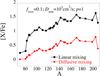 |
Fig. 9 Surface overabundance distributions [X/Fe] for the 28 s-only nuclei at the end of the AGB phase of a 2 M⊙[Fe/H] = −0.5 model star resulting from the LM and DM schemes. In both cases, Dmin = 103 cm2/ s, p = 1 and fover = 0.1. |
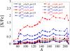 |
Fig. 10 Surface overabundance distributions [X/Fe] for the 28 s-only nuclei at the end of the AGB phase of a 2 M⊙[Fe/H] = −0.5 model star computed with the DM overshoot formalism and 9 different sets of mixing parameters, i.e. Dmin = 103,106, and 109 cm2/ s, p = 1/5,1,5 and fover = 0.1. |
5. S-process in stars of different masses and metallicities
As shown in Sect. 4, the abundance distribution of s-nuclei is rather insensitive to the mixing scheme and parametrisation but the production factors strongly depend on its mathematical formulation. The LM model consistently produces significant surface enrichment while the DM approach requires a fine tuning of the underlying parameters to achieve a similar result. Assuming the production of s-elements is similar, it remains to be seen if the overall abundance distributions obtained using both models are comparable for stars with different initial masses and metallicities. The parameters used are Dmin = 103 cm2/ s, p = 1 for the LM scheme and Dmin = 109 cm2/ s, p = 5 for the DM (fover = 0.1 is taken in both cases). The high value of Dmin = 109 cm2/ s was chosen, so that similar surface enrichments are produced between both schemes, making the comparison easier. We are aware that such a high value is difficult to justify on physical grounds but considering a value lower than Dmin = 107 cm2/ s would reduce the PM zone significantly, leading to a negligible s-process production. Figure 11 shows the mass extent of the PM zone ΔMpmz, s-process region ΔMspro, as defined in Sect. 4.2, and the mass ΔM3DUP of 3DUP material as a function of the pulse number, for a 2 M⊙ model computed with three different initial metallicities [Fe/H] = 0, −0.5 and −1. The decline of the PM and s-process zones with the pulse number is a consequence of the growing core mass which produces a strong gravitational pull and thus a higher compression of the layers located below the convective envelope (see also Cristallo et al. 2009). While the LM models give rise to a rather smooth and constant decrease of the PM and s-process zones, irrespective of the metallicity, significantly larger variations are found with the DM prescription. Again, one can see the correlation between the size of the s-process zone (Fig. 11) and the surface overproduction factors (Fig. 12), except to some extent for the [Fe/H] = −1 model star where the 10-4 ≲ X(H) ≲ 10-3 mass range, neglected in the definition of ΔMspro, may contribute to the s-process nucleosynthesis (Goriely & Mowlavi 2000). As far as the dredge-up mass is concerned, both prescriptions yield rather similar values, at least when the 3DUP efficiency has reached its asymptotic value, that is, after the first three to five thermal pulses depending on the stellar metallicity (Fig. 11).
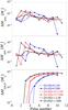 |
Fig. 11 Upper panel: extent of the PM zone ΔMpmz in a 2 M⊙ model as a function of the pulse number for 3 different initial metallicities; [Fe/H] = 0, −0.5 and −1. The LM scheme uses Dmin = 103 cm2/ s, p = 1 and fover = 0.1 and the DM case Dmin = 109 cm2/ s, p = 5 and fover = 0.1. Middle panel: same but for the mass of the s-process zone ΔMspro. Lower panel: same but for the dredged-up mass ΔM3DUP |
The sensitivity of the s-process production on the mixing scheme and initial composition is illustrated in Fig. 12. As can be seen, the final surface enrichment between the two mixing schemes mainly differs in terms of overproduction factors, but also in terms of isotopic and elemental distributions. With our specific choice of parameters, the DM scheme yields similar or even higher s-process overproduction factors than the standard LM parametrization. It remains, however, difficult to reach surface enrichments larger than typically 2 dex. At solar metallicity the s-process surface enrichment is relatively weak, despite the fact that the extent of the s-process zone (Fig. 11) is relatively similar to the other model stars with lower metallicities. This is essentially due to the smaller number and relatively shallower 3DUP episodes found in solar metallicity stars. While six 3DUP are predicted in our 2 M⊙[Fe/H] = 0 model star, nine are found for a metallicity of [Fe/H] = −1. In addition, in the last five thermal pulse-interpulse sequences, the 3DUP of the solar metallicity star drags from 5% to 25% of the thermal pulse material into the envelope, while the 3DUP efficiency reaches more than 35% in the [Fe/H] = −1 model star. This pattern is found to be qualitatively independent of the adopted overshoot model, although quantitatively some minor differences are found.
Some differences in the element distribution can also be found. In particular, when compared with the LM scheme, the DM models tends to give rise to a lower production of light s-elements with respect to the heavy s-elements, as seen in Figs. 12 and 13, and in Table 2. While this difference is marginal in the solar metallicity star, this is particularly clear in the 2 M⊙, [Fe/H] = −1 model star, where a lower 90 ≲ A ≲ 140 distribution by almost 0.5 dex is found with the DM model compared to the LM formulation. The corresponding observational [hs/ls] index, where hs describes the heavy s-elements (Ba, La and/or Nd) abundance and ls the light s-elements (Sr, Y and/or Zr) abundance, can differ by up to 0.2 dex (Table 2). The low production of light s-elements with the DM model is due to the specific profile of the diffusion coefficient obtained with the large p = 5 and Dmin = 109 cm-2/ s values (see Figs. 1 and 5). With these parameters, more weight is given to the layers with proton abundances close to X(H) ≃ 10-3 at the expense of X(H) ≃ 10-2, and as a consequence the production of light elements is reduced with respect to heavy ones (see in particular Fig. 3 of Goriely & Mowlavi 2000).
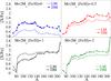 |
Fig. 12 Dependence on stellar metallicity of the final surface overabundance distributions [X/Fe] of the 28 s-only nuclei at the surface of a 2 M⊙ model resulting from the LM scheme with Dmin = 103 cm2/ s, p = 1 and the DM formulation with Dmin = 109 cm2/ s, p = 5. In both cases, fover = 0.1 is taken. Four metallicities [Fe/H] = 0, −0.5, −1 and −2 have been considered. |
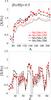 |
Fig. 13 Top panel: as Fig. 12 for the dependence on the stellar mass of the final surface overabundance distribution of s-only nuclei. Stars of 2 and 3 M⊙ with a metallicity [Fe/H] = −0.5 are considered. Lower panel: same as the left panel for the final surface elemental distribution of all elements above Ge. |
We also notice that with decreasing metallicity, the production of heavier elements is favored as a consequence of the lower abundance of iron seed nuclei, hence a larger neutron-to-seed ratio. We note the systematic overproduction of Pb at [Fe/H] ≤ −1 which accounts for Pb-stars (Van Eck et al. 2001), but none of the models studied here can explain some s-process enriched C-enhanced metal-poor stars (Bisterzo et al. 2011; Piersanti et al. 2013) as well as low-metallicity post-AGB stars (e.g., De Smedt et al. 2014, 2016) that are poorly enriched in Pb.
Finally, the effect of varying the initial mass is illustrated in Fig. 13. As confirmed by Table 2, these calculations indicate that, with increasing stellar mass, the [hs/ls] ratio decreases, essentially because of some additional production of light s-elements in hotter thermal pulses. While in our 2 M⊙[Fe/H] = −0.5 model star, Tp does not exceed 3 × 10⁸ K, in the 3 M⊙ model it reaches 3.5 × 10⁸ K, allowing for the activation of the 22Ne(α, n)25Mg reaction in the convective thermal pulse. The [hs/ls] index is found to be smaller by 0.3 (0.2) dex in the 3 M⊙ star with respect to the 2 M⊙ star when adopting the LM (DM) model. Future calculations will explore stellar models within a wider range of masses and metallicities.
Independently of this work, Buntain et al. (2017) investigated the sensitivity of the s-process nucleosynthesis to the proton profile and mass extent of the PM zone. Their approach differs from ours as they perform post-processing calculations in which they impose the proton profile at the time of the 3DUP and the extent of the PM zone ΔMpmz. These authors find that the resulting s-process abundance distribution remains weakly (by more or less 0.2 dex) dependent on the shape of the mixing function, except at low metallicity (Z = 0.0001) where the Pb abundance can be significantly affected. These results are consistent with those presented here, except for the Pb production in metal poor-stars that always remain relatively high in our calculations.
6. Conclusions
Surface [hs/ls] index deduced from the [La/Y] ratio at the end of the evolution of the five model stars studied here and for both LM and DM schemes.
Assuming overshooting below the convective envelope of an AGB stars can be described by an exponential decrease of the diffusion coefficient or equivalently of the convective velocity, we analyzed the impact of two different numerical modeling of the chemical transport on the resulting s-process nucleosynthesis. We have shown that for the same set of parameters, both descriptions give a rather similar abundance distribution of s-only nuclei (though some differences are found in the relative production of light to heavy s-elements), but the surface enrichment can differ drastically. As found by Cristallo et al. (2009), the linear algorithm leads to the formation of a PM zone that can easily account for large surface s-process enrichments. On the other hand, the DM approach requires a quite extreme set of parameters producing diffusion profiles that sharply drop to zero below a threshold value of Dmin ~ 107−109 cm2/s. At this stage, it is however not possible to exclude this set of parameters, nor to favor one prescription over the other. Both schemes are able to phenomenologically simulate the PM of protons inside the C-rich layers. Our exploration of the parameters attests of the difficulty to find a choice of parameters that leads to surface enrichments significantly larger than typically 2 dex for the bulk of s-elements. However, it remains unclear if stars of different masses and metallicities are characterized by similar sets of parameters and if these parameters are constant during the evolution. Furthermore, additional processes induced by gravity waves or rotational mixing can interfere with the s-process nucleosynthesis. Differences in the s-process distributions between the two schemes may be more perceptible in higher mass stars with the LM scheme producing more light s-elements. We also report that, contrary to Battino et al. (2016), our simulations do not show evidence for a strong s-process nucleosynthesis when using their double exponential overshooting prescription. The reason is ascribed to the fact that with this formulation, mixing is still active in the PM zone during the interpulse phase and allows pollution of the -pocket by the  neutron poison.
Available at http://www-astro.ulb.ac.be/Bruslib
Acknowledgments
L.S. and S.G. are FRS-F.N.R.S. research associates.
References
- Angulo, C., Arnould, M., Rayet, M., et al. 1999, Nucl. Phys. A, 656, 3 [NASA ADS] [CrossRef] [Google Scholar]
- Arnould, M., & Goriely, S. 2006, Nucl. Phys. A, 777, 157 [NASA ADS] [CrossRef] [Google Scholar]
- Asplund, M., Grevesse, N., Sauval, A. J., & Scott, P. 2009, ARA&A, 47, 481 [NASA ADS] [CrossRef] [Google Scholar]
- Battino, U., Pignatari, M., Ritter, C., et al. 2016, ApJ, 827, 30 [NASA ADS] [CrossRef] [Google Scholar]
- Bisterzo, S., Gallino, R., Straniero, O., Cristallo, S., & Käppeler, F. 2011, MNRAS, 418, 284 [NASA ADS] [CrossRef] [Google Scholar]
- Buntain, J. F., Doherty, C. L., Lugaro, M., et al. 2017, MNRAS, 471, 824 [NASA ADS] [CrossRef] [Google Scholar]
- Busso, M., Gallino, R., & Wasserburg, G. 1999, ARA&A, 37, 239 [NASA ADS] [CrossRef] [Google Scholar]
- Chieffi, A., Dominguez, I., Limongi, M., & Staniero, O. 2001, ApJ, 553, 1159 [NASA ADS] [CrossRef] [Google Scholar]
- Cristallo, S., Straniero, O., Gallino, R., et al. 2009, ApJ, 696, 797 [NASA ADS] [CrossRef] [Google Scholar]
- De Smedt, K., Van Winckel, H., Kamath, D., et al. 2014, A&A, 563, L5 [NASA ADS] [CrossRef] [EDP Sciences] [Google Scholar]
- De Smedt, K., Van Winckel, H., Kamath, D., et al. 2016, A&A, 587, A6 [NASA ADS] [CrossRef] [EDP Sciences] [Google Scholar]
- Denissenkov, P. A., & Tout, C. A. 2003, MNRAS, 340, 722 [NASA ADS] [CrossRef] [Google Scholar]
- Freytag, B., Ludwig, H.-G., & Steffen, M. 1996, A&A, 313, 497 [Google Scholar]
- Goriely, S. 1999, A&A, 342, 881 [NASA ADS] [Google Scholar]
- Goriely, S., & Mowlavi, N. 2000, A&A, 362, 599 [NASA ADS] [Google Scholar]
- Goriely, S., Hilaire, S., & Koning, A. J. 2008, A&A, 487, 767 [NASA ADS] [CrossRef] [EDP Sciences] [Google Scholar]
- Herwig, F. 2000, A&A, 360, 952 [NASA ADS] [Google Scholar]
- Herwig, F., Blöcker, T., Schönberner, D., & Eid, M. E. 1997, A&A, 324, L81 [NASA ADS] [Google Scholar]
- Herwig, F., Langer, N., & Lugaro, M. 2003, ApJ, 593, 1056 [NASA ADS] [CrossRef] [Google Scholar]
- Herwig, F., Freytag, B., Hueckstaedt, R. M., & Timmes, F. X. 2006, ApJ, 642, 1057 [NASA ADS] [CrossRef] [Google Scholar]
- Herwig, F., Freytag, B., Fuchs, T., et al. 2007, in Why Galaxies Care About AGB Stars: Their Importance as Actors and Probes, eds. F. Kerschbaum, C. Charbonnel, & R. F. Wing, ASP Conf. Ser., 378, 43 [Google Scholar]
- Herwig, F., Woodward, P. R., Lin, P.-H., Knox, M., & Fryer, C. 2014, ApJ, 792, L3 [NASA ADS] [CrossRef] [Google Scholar]
- Iben, I., & Renzini, A. 1982, A&A, 263, L23 [Google Scholar]
- Käppeler, F., Beer, H., & Wisshak, K. 1989, Rep. Prog. Phys., 52, 945 [Google Scholar]
- Karakas, A. I., & Lattanzio, J. C. 2014, PASA, 31, e030 [NASA ADS] [CrossRef] [Google Scholar]
- Lugaro, M., Karakas, A. I., Stancliffe, R. J., & Rijs, C. 2012, ApJ, 747, 2 [NASA ADS] [CrossRef] [Google Scholar]
- Maeder, A., & Meynet, G. 1987, A&A, 182, 243 [NASA ADS] [Google Scholar]
- Marigo, P. 2002, A&A, 387, 507 [NASA ADS] [CrossRef] [EDP Sciences] [Google Scholar]
- Nemeth, Z., Käppeler, F., Theis, C., Belgya, T., & Yates, S. 1994, ApJ, 426, 357 [NASA ADS] [CrossRef] [Google Scholar]
- Nucci, M. C., & Busso, M. 2014, ApJ, 787, 141 [NASA ADS] [CrossRef] [Google Scholar]
- Piersanti, L., Cristallo, S., & Straniero, O. 2013, ApJ, 774, 98 [NASA ADS] [CrossRef] [Google Scholar]
- Reimers, D. 1975, Mem. Soc. Roy. Sci. Liège, 8, 369 [Google Scholar]
- Sallaska, A. L., Iliadis, C., Champagne, A. E., et al. 2013, ApJS, 207, 18 [NASA ADS] [CrossRef] [Google Scholar]
- Siess, L. 2006, A&A, 448, 717 [NASA ADS] [CrossRef] [EDP Sciences] [Google Scholar]
- Siess, L., Dufour, E., & Forestini, M. 2000, A&A, 358, 593 [NASA ADS] [Google Scholar]
- Siess, L., Goriely, S., & Langer, N. 2004, A&A, 415, 1089 [NASA ADS] [CrossRef] [EDP Sciences] [Google Scholar]
- Sparks, W., & Endal, A. 1980, ApJ, 237, 130 [NASA ADS] [CrossRef] [Google Scholar]
- Stancliffe, R. J., Dearborn, D. S. P., Lattanzio, J. C., Heap, S. A., & Campbell, S. W. 2011, ApJ, 742, 121 [NASA ADS] [CrossRef] [Google Scholar]
- Straniero, O., Gallino, R., & Cristallo, S. 2006, Nucl. Phys. A, 777, 311 [NASA ADS] [CrossRef] [Google Scholar]
- Takahashi, K., & Yokoi, K. 1987, At. Data Nucl. Data Tables, 36, 375 [Google Scholar]
- Van Eck, S., Goriely, S., Jorissen, A., & Plez, B. 2001, Nature, 793 [Google Scholar]
- Vassiliadis, E., & Wood, P. R. 1993, ApJ, 413, 641 [NASA ADS] [CrossRef] [Google Scholar]
- Xu, Y., Goriely, S., Jorissen, A., Chen, G., & Arnould, M. 2013a, A&A, 549, A10 [Google Scholar]
- Xu, Y., Takahashi, K., Goriely, S., et al. 2013b, Nucl. Phys. A, 918, 61 [NASA ADS] [CrossRef] [Google Scholar]
- Zamora, O., Abia, C., Plez, B., Domínguez, I., & Cristallo, S. 2009, A&A, 508, 909 [NASA ADS] [CrossRef] [EDP Sciences] [Google Scholar]
All Tables
Extent in mass (in unit of 10-4M⊙) of the PM zone (ΔMpmz) and s-process region (ΔMspro) for the LM and DM models and the different adopted values of the parameters p and Dmin (in cm2/ s). In all cases, fover = 0.1.
Surface [hs/ls] index deduced from the [La/Y] ratio at the end of the evolution of the five model stars studied here and for both LM and DM schemes.
All Figures
|
Fig. 1 Profile of the overshoot diffusion coefficient Dover as a function of the reduced depth z/z∗ for different values of p and assuming Dcb = 1016 cm2/ s, Dmin = 103 cm2/ s. |
| In the text | |
|
Fig. 2 Upper panel: Kippenhahn diagram of our 2 M⊙[Fe/H] = −0.5 during the first dredge-up and core He burning phases; the green and blue dotted lines delineate the region of maximum nuclear energy production by H- and He-burning, respectively. Middle panel: evolution of the central neutron density Nn, central 13C mass fraction (×106) and neutron exposure τ. Lower panel: evolution of the central temperature Tc and density ρc. |
| In the text | |
|
Fig. 3 Final overproduction factors [X/Fe] of all stable nuclei with A ≥ 30 (full squares) at the center of our 2 M⊙[Fe/H] = −0.5 model star at the end of core helium burning. The s-only nuclei are shown by red diamonds connected by a solid line. The vertical line depicts the total decay of the s-only nucleus 123Te. |
| In the text | |
|
Fig. 4 Left panels: proton mass fraction (bottom panel) and diffusion coefficient (top panel) profiles below the convective envelope resulting from the LM scheme with overshoot parameters fover = 0.1, Dmin = 103 cm2/ s and 3 values of p = 1/2, 1, 5. Right panels: same but for fover = 0.1, p = 1 and 4 values of Dmin = 101.9 cm2/ s. The profiles were taken when the convective envelopes reaches its deepest inward extent. For display convenience, the Dmin = 109 profiles have been shifted outward by 0.00085 M⊙. |
| In the text | |
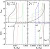 |
Fig. 5 As Fig. 4 but for the diffusive treatment (DM) of overshooting. |
| In the text | |
|
Fig. 6 Overabundance distributions [X/Fe] for the 28 s-only nuclei inside a region of 0.01 M⊙ around Mr = 0.595−0.605M⊙ at the end of the 8th interpulse of our 2 M⊙[Fe/H] = −0.5 model star. The results are shown for different LM conditions, i.e. different values of p (upper panel) or Dmin (in cm2/s; lower panel); in all cases, fover = 0.1 is assumed. |
| In the text | |
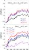 |
Fig. 7 As Fig. 6 for the s-process distributions obtained with the DM model. |
| In the text | |
|
Fig. 8 Ratio of the nuclei mass fraction after (Xconv) and before (Xrad) the 9th thermal pulse of our 2 M⊙[Fe/H] = −0.5 model star. Open and filled squares represent stable and s-only nuclei, respectively. |
| In the text | |
|
Fig. 9 Surface overabundance distributions [X/Fe] for the 28 s-only nuclei at the end of the AGB phase of a 2 M⊙[Fe/H] = −0.5 model star resulting from the LM and DM schemes. In both cases, Dmin = 103 cm2/ s, p = 1 and fover = 0.1. |
| In the text | |
|
Fig. 10 Surface overabundance distributions [X/Fe] for the 28 s-only nuclei at the end of the AGB phase of a 2 M⊙[Fe/H] = −0.5 model star computed with the DM overshoot formalism and 9 different sets of mixing parameters, i.e. Dmin = 103,106, and 109 cm2/ s, p = 1/5,1,5 and fover = 0.1. |
| In the text | |
|
Fig. 11 Upper panel: extent of the PM zone ΔMpmz in a 2 M⊙ model as a function of the pulse number for 3 different initial metallicities; [Fe/H] = 0, −0.5 and −1. The LM scheme uses Dmin = 103 cm2/ s, p = 1 and fover = 0.1 and the DM case Dmin = 109 cm2/ s, p = 5 and fover = 0.1. Middle panel: same but for the mass of the s-process zone ΔMspro. Lower panel: same but for the dredged-up mass ΔM3DUP |
| In the text | |
|
Fig. 12 Dependence on stellar metallicity of the final surface overabundance distributions [X/Fe] of the 28 s-only nuclei at the surface of a 2 M⊙ model resulting from the LM scheme with Dmin = 103 cm2/ s, p = 1 and the DM formulation with Dmin = 109 cm2/ s, p = 5. In both cases, fover = 0.1 is taken. Four metallicities [Fe/H] = 0, −0.5, −1 and −2 have been considered. |
| In the text | |
|
Fig. 13 Top panel: as Fig. 12 for the dependence on the stellar mass of the final surface overabundance distribution of s-only nuclei. Stars of 2 and 3 M⊙ with a metallicity [Fe/H] = −0.5 are considered. Lower panel: same as the left panel for the final surface elemental distribution of all elements above Ge. |
| In the text | |
Current usage metrics show cumulative count of Article Views (full-text article views including HTML views, PDF and ePub downloads, according to the available data) and Abstracts Views on Vision4Press platform.
Data correspond to usage on the plateform after 2015. The current usage metrics is available 48-96 hours after online publication and is updated daily on week days.
Initial download of the metrics may take a while.