| Issue |
A&A
Volume 608, December 2017
|
|
|---|---|---|
| Article Number | A47 | |
| Number of page(s) | 15 | |
| Section | Stellar structure and evolution | |
| DOI | https://doi.org/10.1051/0004-6361/201730922 | |
| Published online | 05 December 2017 | |
ULX spectra revisited: Accreting, highly magnetized neutron stars as the engines of ultraluminous X-ray sources
1 CNRS, IRAP9 Av. colonel Roche, BP 44346, 31028 Toulouse Cedex 4, France
2 Université de Toulouse, UPS-OMP, IRAP, 31400 Toulouse, France
e-mail: This email address is being protected from spambots. You need JavaScript enabled to view it.
3 Max-Planck-Institut für Extraterrestrische Physik, Giessenbachstraße, 85748 Garching, Germany
4 INAF/Osservatorio Astronomico di Cagliari, via della Scienza 5, 09047 Selargius (CA), Italy
Received: 3 April 2017
Accepted: 13 October 2017
Abstract
Aims. In light of recent discoveries of pulsating ultraluminous X-ray sources (ULXs) and recently introduced theoretical schemes that propose neutron stars (NSs) as the central engines of ULXs, we revisit the spectra of eighteen well known ULXs, in search of indications that favour this newly emerging hypothesis.
Methods. We examine the spectra from high-quality XMM-Newton and NuSTAR observations. We use a combination of elementary black body and multicolour disk black body (MCD) models, to diagnose the predictions of classic and novel theoretical models of accretion onto NSs. We re-interpret the well established spectral characteristics of ULXs in terms of accretion onto lowly or highly magnetised NSs, and explore the resulting parameter space for consistency.
Results. We confirm the previously noted presence of the low-energy (≲6 keV) spectral rollover and argue that it could be interpreted as due to thermal emission. The spectra are well described by a double thermal model consisting of a “hot” (≳1 keV) and a “cool” (≲0.7 keV) multicolour black body (MCB). Under the assumption that the “cool” MCD emission originates in a disk truncated at the neutron star magnetosphere, we find that all ULXs in our sample are consistent with accretion onto a highly magnetised (B ≳ 1012 G) neutron star. We note a strong correlation between the strength of the magnetic field, the temperature of the “hot” thermal component and the total unabsorbed luminosity. Examination of the NuSTAR data supports this interpretation and also confirms the presence of a weak, high-energy (≳15 keV) tail, most likely the result of modification of the MCB emission by inverse Compton scattering. We also note that the apparent high-energy tail, may simply be the result of mismodelling of MCB emission with an atypical temperature (T) versus radius (r) gradient, using a standard MCD model with a fixed gradient of T ~ r-0.75.
Conclusions. We have offered a new and robust physical interpretation for the dual-thermal spectra of ULXs. We find that the best-fit derived parameters of our model, are in excellent agreement with recent theoretical predictions that favour super-critically accreting NSs as the engines of a large fraction of ULXs. Nevertheless, the considerable degeneracy between models and the lack of unequivocal evidence cannot rule out other equally plausible interpretations. Deeper broadband observations and time-resolved spectroscopy are warranted to further explore this newly emerging framework.
Key words: X-rays: binaries / accretion, accretion disks
© ESO, 2017
1. Introduction
Ultraluminous X-ray sources (ULXs) are off-nuclear, extragalactic X-ray sources with isotropic luminosities that exceed the Eddington limit for a stellar-mass black hole (BH) (MBH ≲ 20 M⊙: see Feng & Soria 2011, and references therein; and also Bachetti 2016; and Kaaret et al. 2017, for up-to-date and comprehensive reviews). It was initially suggested that ULXs were rare instances of intermediate-mass BHs accreting at sub-Eddington rates (Colbert & Mushotzky 1999; Makishima et al. 2000; Kaaret et al. 2001; Miller et al. 2003); essentially a scaled-up version of standard galactic BH X-ray binaries (BH-XRBs). However, it was quickly realised that a considerable fraction (if not all) of the ULX population can be powered by stellar-mass BHs accreting at super-Eddington rates (e.g. Gao et al. 2003; Gilfanov et al. 2004; Roberts et al. 2004; Poutanen et al. 2007; King 2009). Furthermore, the astounding discovery of a pulsating ULX (PULX: Bachetti et al. 2014) demonstrated that ULXs can be powered by neutron stars (NSs). After the initial discovery by Bachetti et al., two more PULXs have been detected (Israel et al. 2017; Fürst et al. 2016).
The discovery of NS-ULXs provided further support to the scenario of super-Eddington accretion onto a stellar-mass compact object as the power source of ULXs, but also posed the crucial question of the potential prevalence of NSs as the engines of ULXs. Indeed, it has been known for some time that most of the ULXs do not transition through the phenomenological states of standard BH-XRBs, that is, spectral transitions between hard and soft states and the appearance and quenching of relativistic jets (for a review of spectral and temporal properties of NS- and BH-XRBs see e.g. Barret 2001; Remillard & McClintock 2006; Done et al. 2007; Gilfanov 2010). While some ULXs exhibit significant luminosity and spectral variations (e.g. Swartz et al. 2004; Sutton et al. 2013; Feng et al. 2016), they do not transition between the markedly different and characteristic hard and soft spectral states of nominal, sub-Eddington BH-XRBs (e.g. Berghea et al. 2008; Grisé et al. 2010; Sutton et al. 2013). Interestingly two hyperluminous X-ray sources (HLXs) – which have luminosities exceeding ~1041erg s-1 and are strong IMBH candidates – seem to follow the transition pattern of stellar-mass BH-XRBs (ESO 243-49 HLX-1: Godet et al. 2009; Servillat et al. 2011; Webb et al. 2012; or M82 X-1: Feng & Kaaret 2010). In this work we only consider ULXs that are limited to luminosities ≲ 1041 erg/s.
In addition to the lack of state transitions, the spectra of numerous ULXs are significantly different from the typical spectra of BH-XRBs. More specifically, the majority of ULX spectra feature a notable spectral curvature above ~ 6 keV (e.g. Stobbart et al. 2006; Gladstone et al. 2009; Sutton et al. 2013). It has been proposed that perhaps the unusual spectra of ULXs correspond to a novel state of super-critical accretion, dubbed the ultralumimous state (Gladstone et al. 2009). In subsequent works it was posited that ULX spectra can be empirically classified into three classes based on their spectral shape: singly peaked broadened disc (BD) class and two-component hard ultraluminous (HUL) and soft ultraluminous (SUL) states (Sutton et al. 2013). Recognising the physical mechanisms underlying the observed spectral characteristics of ULXs is a crucial step towards understanding accretion at super-Eddington states but also determining the nature of their accretor.
In the recent months leading to this publication, an increasing number of compelling theoretical considerations – that point to NSs as plausible engines behind ULX emission – have been put forward by numerous authors (e.g. King & Lasota 2016; King et al. 2017; Mushtukov et al. 2017). Motivated by these findings and the apparent spectral and temporal similarities between ULXs and NS-XRBs we decided to revisit the spectra of known ULXs, in search of indications that may favour this newly emerging trend. More specifically, we ask whether the curvature of ULX spectra is due to hot thermal emission, rather than a hard power law with a cutoff at an improbably low energy and whether this can be physically interpreted in terms of emission from a super-critically accreting NS. To investigate this hypothesis, we have selected eighteen well known ULXs that have been studied by multiple authors in the past and were also included in the samples used in the seminal works of Stobbart et al. (2006) and Sutton et al. (2013), in which the spectral shape of ULXs was standardised and classified observationally. Below (Sect. 2) we briefly present the different interpretations of the spectral curvature in ULXs, the latest theoretical arguments for the nature of their central engine and the motivation behind our choice to revisit the spectra of known ULXs. In Sect. 3 we present the details of our data analysis and in Sect. 4 we discuss our findings and their implications with regard to the nature of the accretor in our sample and in ULXs in general.
2. Origin of the curvature in the spectra of ULXs
2.1. Optically thick, warm corona
Nominal BH-XRBs exhibit a power-law shaped tail towards high energies, during all spectral states. More specifically, during episodes of low-luminosity-advection-dominated accretion (also known as a hard state) the spectrum is dominated by a hard power law (spectral index of up to ~1.5) with an exponential cutoff at ~100–200 keV, while in the high-luminosity soft state, the power-law component becomes, less prominent and softer (spectral index exceeding ~2), but without an observable spectral cutoff (e.g. Barret 2001; Gallo et al. 2003; Narayan 2005; Remillard & McClintock 2006; Done et al. 2007; Gilfanov 2010). As discussed above, the spectra of many ULXs (including all sources studied in this work) feature a spectral curvature and an abrupt drop in spectral counts at considerably lower energies than standard BH-XRBs. The spectral roll-over in ULXs was detected in XMM-Newton data of numerous sources (e.g. Stobbart et al. 2006; Sutton et al. 2013) and was subsequently confirmed with the NuSTAR telescope (e.g. Bachetti et al. 2013; Walton et al. 2014, 2015; Fürst et al. 2017). It is often observed as low as ~3 keV.
In the past, many authors have modelled the unusual low-energy curvature of ULX spectra (including the ones revisited here) using a power-law spectrum with a low-energy cutoff and a relatively large e-folding energy (e.g. Stobbart et al. 2006; Roberts 2007; Gladstone et al. 2009; Sutton et al. 2013). The uncommonly low-energy cutoff, is often linked to the presence of a corona of hot, thermal electrons with an unusually high Thomson scattering optical depth. Namely, multiple authors have considered that the shape of the high-energy part of the spectrum is the result of thermal Comptonisation of soft (hν < 0.5 keV) photons, by a corona of thermal electrons with an optical depth that often exceeds τT ≈ 20 (e.g. Stobbart et al. 2006; Roberts 2007; Gladstone et al. 2009; Pintore & Zampieri 2012; Sutton et al. 2013; Pintore et al. 2014). While this configuration successfully reproduces the observed spectral shapes, its feasibility under realistic circumstances in the vicinity of critically accreting X-ray binaries may be problematic. More specifically, the high scattering depth combined with the increased photon density will pose a significant burden to the coronal thermalisation. This can be illustrated in the following simplified example, where we consider cooling due to inverse Compton (IC) scatterings and Coulomb collisions as the sole thermalisation mechanism. The cooling rate of thermal electrons due to multiple IC scatterings by photons with hν ≪ kTe depends strongly on the scattering optical depth of the corona, that is, the cooling timescale for large optical depth is (e.g. Rybicki & Lightman 1979) 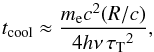 (1)where me is the electron mass and R/c the characteristic source size, which can be inferred from variability considerations. It is obvious from Eq. (1) alone that for the values of τT reported in these works, Compton cooling will be very rapid, that is, tcool ≪ R/c. Below we illustrate that the cooling timescale will be too small to allow for electron thermalisation.
The thermalisation will occur primarily through energy exchange between high-energy electrons and the thermal background of electrons and protons in the coronal plasma. For a high scattering optical depth (i.e. τT > 5), one can plausibly assume that the main mechanism for the energy exchange will be Coulomb interactions between electrons and electrons, and electrons and protons, ignoring, for example, collective interactions between particles (e.g. Begelman & Chiueh 1988). If the relativistic electrons exchange energy more rapidly than they cool due to multiple scatterings, then the plasma will thermalise efficiently. The timescale of the Coulomb energy exchange will be 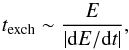 (2)where E is the electron energy and dE/dt is the Coulomb cooling rate (Gould 1975; Frankel et al. 1979; Coppi & Blandford 1990). For relativistic electrons the Coulomb rate can be rewritten as (see also Coppi 1999),
 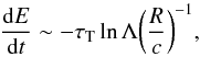 (3)where lnΛ is the usual Coulomb logarithm. From the above approximations, it becomes evident that while the Coulomb cooling becomes more rapid, as optical depth increases (texch ~ τT-1), the τT-2 dependence of the Compton cooling timescale, results in a corona in which energetic photons cool down before they can thermalise. As τT increases, a thermal corona becomes more and more difficult to sustain. The problem of coronal thermalisation is well known, and it can also become significant in the low τT regime (e.g. Coppi 1999, and references therein), particularly for hot (kTe ≳ mec2) coronas. As a result, the presence of hybrid thermal/non-thermal electron distributions (e.g. Coppi 1999; Belmont et al. 2008; Malzac & Belmont 2009) is usually assumed. However, the high-scattering optical depths that were claimed in earlier ULX literature (e.g. Stobbart et al. 2006; Roberts 2007; Gladstone et al. 2009; Sutton et al. 2013), present major sustainability issues even when considering hybrid, “warm” coronas with lower electron temperatures. It is only under very tight restrictions that coronas with τT > 5 can be sustained (e.g. Różańska et al. 2015). We must stress here, that the issues concerning the physical plausibility of the optically thick corona model have been noted by the community since relatively early on (e.g. Middleton et al. 2011; Kajava et al. 2012), with the majority of later works, only using the power law with the exponential cutoff as an empirical description of the hard emission of ULXs, rather than a physical interpretation.
2.2. Optically thick winds
The most widely accepted interpretation of the spectral curvature of ULXs invokes the presence of strong, optically thick winds. Namely, under the assumption that ULXs are accreting BHs in the super-Eddington regime, then the spectral shape of the emission may be strongly influenced by the presence of massive, optically thick outflows. King & Pounds (2003) and Poutanen et al. (2007) argued that the curvature of the spectra (of at least some) ULXs can be interpreted in terms of reprocessing of the primary emission in the optically thick wind. In this scenario the soft thermal emission is associated with the wind itself, and the hard emission is also thermal and originates in the hot, innermost parts of an accretion disk. Kajava & Poutanen (2009) followed up the predictions of Poutanen et al. (2007) and by studying the spectra of eleven known ULXs they claimed that the temperature of the soft thermal component decreased with its luminosity (i.e. Lsoft ~ Tin-3.5), in agreement with the prediction for emission from an optically thick wind. However, subsequent studies by (e.g. Miller et al. 2013) found that the luminosity of the soft component correlates positively with temperature, approximately following the Lsoft ~ Tin4 relations expected for standard accretion disks. However, in a recent study of numerous long-term observations of HO IX X-1, Luangtip et al. (2016) show that – with increasing luminosity – the source spectra evolve from a two-component spectrum to a (seemingly) single-component, thermal-like spectrum. The authors argue that the apparent heating of the soft-disk component may be model dependent, an artifact caused by neglecting to properly account for the evolving spectra.
In addition to the prediction of the ULX spectral shape, the optically thick wind model also offers an interpretation for the short-timescale variability noted in many sources (e.g. Sutton et al. 2013). More specifically, Middleton et al. (2015a) combined the arguments of King & Pounds (2003) and Poutanen et al. (2007) with predictions for wind inhomogeneity (e.g. Takeuchi et al. 2013) and mass-accretion rate fluctuations (e.g. Ingram & van der Klis 2013) to account for spectral and timing variability of nine ULXs. The authors made a well-founded case for super-Eddington accretion onto stellar-mass BHs as the driving force behind ULXs. In this scheme the fractional variability noted by previous authors is explained in terms of a “clumpy” wind partially obscuring the hard component, which appears to fluctuate. In the same context the different empirical states indicated by Sutton et al. (2013) are the result of different orientations between the observer and the disk/wind structure (see Fig. 1 of Middleton et al. 2015a). Building on these considerations several authors (e.g. Walton et al. 2014, 2015; Luangtip et al. 2016) have modelled ULX spectra extracted from XMM-Newton and NuSTAR data using a dual thermal model, in which the soft thermal emission is attributed to the optically thick wind and the hotter component to emission from the inner parts of a hot accretion disk. The presence of the strong outflows are also supported by the uniform optical counterparts of numerous ULXs, which indicate a hot wind origin (e.g. Pakull & Mirioni 2002; Fabrika et al. 2015), but also the presence of wind or jet blown, radio “bubbles” around some ULXS (e.g. Pakull & Mirioni 2003; Soria et al. 2006; Cseh et al. 2012). The strongest indication of an outflow lies in the discovery of soft X-ray spectral residuals near ~ 1 keV (e.g. Middleton et al. 2014, 2015b; Pinto et al. 2016, 2017), which have been interpreted as a direct signature of their presence. While broad emission- and absorption-like residuals near the ~ 1 keV mark have been observed in the spectra of numerous NS- and BH-XRBs during different states and at different mass accretion rates (e.g. Boirin & Parmar 2003; Díaz Trigo et al. 2006; Ng et al. 2010; Kolehmainen et al. 2014), the absorption lines detected in the spectra of NGC 1313 X-1 and NGC 5408 X-1 (Pinto et al. 2016), and more recently in NGC 55 ULX (Pinto et al. 2017), seem to be strongly blue-shifted, indicating outflows with velocities reaching 0.2c.
2.3. The case of accreting neutron stars
The recent discoveries of the three PULXs, has established the fact that ULXs can be powered by accretion onto NSs. This realisation is perhaps not surprising, considering that a mechanism that allows accretion at super-Eddington rates onto highly magnetised (B ≳ 1012 G) NSs has been put forward since the late seventies (Gnedin & Sunyaev 1973; Basko & Sunyaev 1975, 1976). However, these works were not aimed at discussing super-Eddington accretion in the context of ULXs. The authors were attempting to resolve the complications that arise from the fact that when material is accreted onto a very small area on the surface of the NS the Eddington limit is considerably lower than the ~ 1.8 × 1038 erg/s, which corresponds to isotropic accretion onto a NS. Therefore, persistent X-ray pulsars with luminosities exceeding a few 1037 erg/s, were in fact breaking the (local) Eddington limit. More specifically, in high-B accreting NSs, the accretion disk is interrupted by the magnetic field near the magnetospheric radius, at which point the accreted material is guided by the magnetic field lines onto a small area centered around the NS magnetic poles (e.g. Pringle & Rees 1972; Romanova et al. 2012). The resulting formation is known as an accretion column. Due to the high anisotropy of the photon–electron scattering cross-section in the presence of a strong magnetic field (Canuto et al. 1971; Lodenquai et al. 1974), the emission from the accretion column is concentrated in a narrow (“pencil-”) beam, which is directed parallel to the magnetic field lines (and hence the magnetic field axis, Basko & Sunyaev 1975). However, at high mass-accretion rates a radiation dominated shock is formed at a few km above the surface of the NS. As accretion rate exceeds a critical value (corresponding to a critical luminosity of ~ 1037 erg/s, e.g. Basko & Sunyaev 1976; Mushtukov et al. 2015b), the accretion funnel is suffused with high-density plasma which is gradually sinking in the gravitational field of the NS (Basko & Sunyaev 1976; Wang & Frank 1981). As a result, the accretion funnel, in the direction parallel to the magnetic field axis, becomes optically thick and the emerging X-ray photons mostly escape from its – optically thin – sides, in a “fan-beam” pattern (see e.g. Fig. 1 Schönherr et al. 2007). In recent refinements of this mechanism, it has been demonstrated that depending on the magnetic field strength and the pulsar spin it can facilitate luminosities of the order of 1040 erg/s (Mushtukov et al. 2015a).
Observations of multiple X-ray pulsars have yielded an empirical description of the primary emission of the accretion column as a very hard power law (spectral index ≲ 1.8) with a low-energy (≲ 10 keV) cutoff (e.g. Caballero & Wilms 2012). While a general, self consistent description of the spectral shape of the accretion column emission has not been achieved yet, several authors have attempted to reproduce it (e.g. Nagel 1981; Meszaros & Nagel 1985; Burnard et al. 1991; Hickox et al. 2004; Becker & Wolff 2007). More specifically, Becker & Wolff (2007) have reproduced the spectrum, assuming bulk and thermal Comptonisation of seed Bremsstrahlung, black body and cyclotron photons.
While, in the high-field regime, super-Eddington accretion can be efficiently sustained, lowly magnetised NSs can only reach moderately super-Eddington luminosities and only in the soft state of the so-called Z-sources (e.g. Muno et al. 2002; Done et al. 2007; Lin et al. 2009). When the accretion rate reaches and exceeds the Eddington limit, strong outflows are expected to inhibit higher accretion rates. Nevertheless, in a recent publication, King & Lasota (2016) argue that super-Eddington accretion onto lowly magnetised NSs can be maintained – along with powerful outflows – in a similar fashion to super-Eddington accretion onto BHs (King et al. 2001). Therefore, a considerable fraction of (non-pulsating) ULXs may be the result of beamed emission from NSs with relatively weak magnetic fields (B < 1011 G), accreting at high mass-transfer rates.
Intriguingly, one of the first (Mitsuda et al. 1984) and most frequently observed spectral characteristics associated with the soft state of Z-sources is the presence of two thermal components (e.g. White et al. 1988; Mitsuda et al. 1989; Barret 2001; Lin et al. 2007; Revnivtsev et al. 2013). The “cool” thermal component most likely originates in a thin Shakura & Sunyaev disk and the additional “hot” thermal component corresponds to emission produced in hot optically thick plasma on the surface of the NS, known as a boundary layer (Sunyaev & Shakura 1986; Sibgatullin & Sunyaev 2000). Therefore, the presence of a dual thermal spectrum in XRBs strongly suggests emission from a solid surface, indicating a lowly magnetised NS. Nevertheless, in a new publication by Mushtukov et al. (2017) it is argued that in accreting high-B NSs, the normally optically thin (e.g. Basko 1980; Nagase et al. 1992; Ebisawa et al. 1996) material trapped in the Alfvén surface becomes optically thick as the luminosity exceeds ~ 5 × 1039 erg/s. The emission of the resulting structure will have a quasi-thermal spectrum at temperatures exceeding 1 keV. Combined with the soft thermal emission from a truncated accretion disk, the spectra of highly magnetised NSs may also feature the same dual thermal shape as high-state Z-sources (Mushtukov et al. 2017, see more details in Sects. 3 and 4). Based on these considerations, it becomes apparent that the reanalysis of ULX spectra is warranted. To this end, we explore the relevance of models, usually implemented in the modelling of emission from NS-XRBs, in the context of ULXs. More importantly, we investigate whether or not our best-fit models yield parameter values that are physically meaningful and in accordance with the predictions for the emission from ULXs.
Observation log.
3. Spectral extraction and data analysis
We have analysed archival XMM-Newton observations of eighteen ULXs presented in Table 1. We have selected sources that have been studied extensively in the past and are confirmed ULXs. Furthermore, specific datasets were selected to have a sufficient number of counts to allow robust discrimination between the different models used to describe their spectral continuum. Except for these conditions, sources were chosen randomly. Therefore, the ULX sample analysed in this work is not complete. Nevertheless, the purpose of this work is not to revisit the entire ULX catalogue, but to demonstrate that a significant fraction of ULXs follow a specific pattern (presented below). For this purpose, our source sample is sufficiently extensive. For six of these sources we also analysed archival NuSTAR data.
3.1. XMM-Newton spectral extraction
For the XMM-Newton data, we only considered the EPIC-pn detector, which has the largest effective area of the three EPIC detectors, in the full 0.3–10 keV bandpass, and registered more than ~1000 photons for each of the observations considered, thus providing sufficient statistics to robustly discriminate between different spectral models while ensuring simplicity and self-consistency in our analysis. Therefore the following description of data analysis refers only to this instrument. The data were handled using the XMM-Newton data analysis software SAS version 15.0.0. and the calibration files released1 on January 22, 2016. In accordance with the standard procedure, we filtered all observations for high background-flaring activity, by extracting high-energy light curves (10 <E < 12 keV) with a 100 s bin size. By placing appropriate threshold count rates for the high-energy photons, we filtered out time intervals that were affected by high particle background. During all observations pn was operated in Imaging Mode. In the majority of our sources, spectra were extracted from a circular region with a radius >35′′ centred at the core of the point spread function (psf) of each source. We thus ensured the maximum encircled energy fraction2 within the extraction region. This was not possible in the case of NGC 4861 ULX1, M81 X-6, and NGC 253 ULX2 where we used spectral extraction apertures of 18″, 13.8′′ and 12.5′′ in order to avoid contamination by adjacent sources or due to the proximity of our source to the edge of the chip3. The extraction and filtering process followed the standard instructions provided by the XMM-Newton Science Operations Centre (SOC4). More specifically, spectral extraction was done with SAS task evselect using the standard filtering flags (#XMMEA_EP && PATTERN<=4 for pn), and SAS tasks rmfgen and arfgen were used to create the redistribution matrix and ancillary file, respectively. All spectra were regrouped to have at least 25 counts per bin and analysis was performed using the xspec spectral fitting package, version 12.9.0 (Arnaud 1996).
3.2. NuSTAR spectral extraction
The NuSTAR data were processed using version 1.6.0 of the NuSTAR data analysis system (NuSTAR DAS). We downloaded all public NuSTAR datasets using the heasarc_pipeline scripts (Multimission Archive TeamOAC, in prep.). These have already been processed to obtain L1 products. We then ran nuproducts using a 50′′ extraction region around the main source and a 50–80′′ extraction region for background, in the same detector as the source when possible, as far as we could to avoid contributions from the point-spread function (PSF) wings. We applied standard PSF, alignment, and vignetting corrections. Spectra were rebinned in order to have at least 30 counts per bin to ensure the applicability of the χ2 statistics. All sources in our sample dominate the background up to 20–30 keV. The models we use are relatively simple, and the physical interpretation does not change considerably for a change of best-fit parameters of 10−20%, and so we do not need an extremely precise modelling of the background.
3.3. Spectral analysis
3.3.1. XMM-Newton
The spectral continuum was modelled twice, firstly using a combination of a multicolour disk black body (MCD) and a black body component (diskbb+bbody), with the black body (bbody) acting as the hot thermal component and secondly using two MCD components (diskbb+diskbb). The first model was used because it is the most widely used model describing the spectra of NS-XRBs in the high-accretion, “soft” state. Our choice for the second model was based on the recent theoretical predictions by Mushtukov et al. (2017), where it is argued that critically accreting NSs with a high magnetic field (i.e. B ≳ 1012 G) can become engulfed in an optically thick toroidal envelope which is the result of accreting matter moving along the magnetic field lines. Emission from the optically thick envelope is predicted to have a multicolour black body spectrum, with a temperature exceeding ~1 keV (more details in Sect. 4). We model this hot thermal emission using the diskbb model because it is the simplest and most reliable multi-temperature black body model in xspec; however we stress that we do not expect this emission to originate from a disk. Therefore, the inner disk radius corresponding to the hot diskbb component has no physical meaning and is not tabulated. In both models the cool disk component is modelled as a geometrically thin, optically thick Shakura & Sunyaev (1973) disk, which is expected to extend inwards until it reaches the surface of the NS, unless it is disrupted by strong outflows or a strong magnetic field (more details in Sect. 4). We did not model intrinsic and/or host galaxy absorption separately from the Galactic absorption, but used one component for the total interstellar absorption, which was modelled using tbnew_gas, the latest improved version of the tbabs X-ray absorption model (Wilms et al. 2011).
Best fit parameters of the dual MCD model for the XMM-Newton observations.
For the dual MCD model, we assume that the disk becomes truncated at approximately the magnetospheric radius at which point the material follows the magnetic field lines to form the hypothetical envelope. Under this assumption, we also estimate the strength of the magnetic field (B), assuming that the inner radius of the “cool” diskbb coincides with the magnetospheric radius (Rmag) and using the expression for Rmag given by Lai (2014; see also Eq. (1) from Mushtukov et al. 2017). The complete xspec model used in the spectral fits is tbnew_gas(cflux*diskbb + cflux*(diskbb or bbody)), where cflux is a convolution model that is used to calculate the flux of the two thermal components. Some of the sources exhibited strong residuals in the 0.5–1.2 keV region, commensurate with X-ray emission lines from hot, optically thin plasma. The emission features were modelled using the mekal model, which models the emission spectrum of a hot diffuse gas. The best fit parameters of the continuum were not sensitive to the modelling of these features (e.g. using a Gaussian instead of mekal), however they are strongly required by the fit (δχ2 > 15 for two d.o.f. in all sources). More specifically, plasma temperature was ~0.92 keV for Ho IX X-1, ~1.09 keV for M81 X-6, ~0.95 keV for M83 ULX, ~0.40 keV for NGC 4736 ULX, and ~1.08 keV for NGC 5204 X-1. While soft X-ray atomic features may be crucial to our understanding of the nature of ULXs (namely, the presence of strong winds and the chemical composition of the accreted material, e.g.: Middleton et al. 2015a,b; Pinto et al. 2016), they are not the focus of this work and are only briefly discussed in Sect. 4, but not studied further.
Given the high (≳ 1 keV) temperatures of the hot thermal component in both double-thermal models, it is expected that electron scattering will have a significant effect on the resulting spectrum, as it becomes comparable to free-free absorption. Therefore, the actual emission will be radiated as a “diluted” black body, which when modelled using a prototypical thermal model like diskbb or bbody will result in temperature and radius estimations that deviate from their “true” values. This issue is commonly addressed by considering a correction factor (fcol) that approximately accounts for the spectral modification (London et al. 1986; Lapidus et al. 1986; Shimura & Takahara 1995); this factor is often referred to as a colour correction factor and detailed calculations, combined with multiple observations have demonstrated that it depends weakly on the size5 of the emitting region and the mass accretion rate (e.g. Shimura & Takahara 1995). Therefore in the first approximation it can be considered independent of these parameters and its value is estimated between ~ 1.5 and ~2.1 (e.g. Zimmerman et al. 2005, and references therein). The colour correction factor affects both the temperature and normalisation of the thermal models (i.e. diskbb and bbody), with the corrected values given by  (4)and
 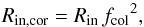 (5)where T is the temperature of the MCD component and Rin is the inner radius. Although the spectral hardening effects are expected to be noticeable, particularly in the hot thermal component, we have decided not to include the colour correction in any of our calculations and to tabulate and plot the values of all quantities of interest as provided by our best fits. The reader is, however, advised to note that the value of our results may vary by a value of ~fcol.
The value of the inferred inner disk radius is also dependent on the viewing angle (i) of the accretion disk (i.e.  ). This dependence may become important in the estimation of Rin if the accretion disk is viewed at a large inclination angle (i.e. edge-on view). Nevertheless, since we have no indications for a high viewing angle (e.g. dips6 in their light curves or spectral absorption features resulting from an edge-on view of the accretion disk atmosphere) in any of our sources, we have selected a value of i = 60deg for all sources in our list.
All best fit values for the absorbed dual-MCD model together with the estimations for the magnetic field and their classification, as proposed by Sutton et al. (2013), are presented in Table 2. The values for the absorbed MCD/black body model are presented in Table 4. In Table 4 we also provide the estimations of the “spherization” radius (Shakura & Sunyaev 1973) of each source. Lastly, we note that the χ2 values from the tbnew_gas*(diskbb+bbody) fits were similar, albeit moderately higher than those of the dual MCD model and with moderately lower temperature of the hot component (kTBB between ~0.9 keV and ~2.2 keV).
3.3.2. NuSTAR
In the NuSTAR spectra we ignored all channels below 4 keV, and thus we did not require the addition of the cool thermal component. The primary spectral component used to model all spectra is again a multicolour disk black body (diskbb), the “hot” thermal component from the XMM-Newton fits. Furthermore, we also look for the presence of a potential hard, non-thermal tail, which is usually detected in most XRBs, even in the soft state. A simultaneous broadband fit of the combined NuSTAR plus XMM-Newton spectra is not explored in this paper. Recent, rigorous works have extensively studied the XMM-Newton (or Swift) + NuSTAR data that we revisit here (Ho II X-1: Walton et al. 2015; HoIX X-1: Luangtip et al. 2016; IC 342 X-1: Rana et al. 2015; NGC 1313 X-1, X-2: Bachetti et al. 2013; NGC 5907 X-1: Fürst et al. 2017) and have noted the presence of a spectral shape that can be modelled either as a hot thermal component or sharp cutoff with an additional, weak power-law tail. In this paper we do not seek to reproduce these analyses, but to discuss a possible novel interpretation of the spectral shape. The NuSTAR data are used with the purpose of confirming (or dismissing) the presence of these components in a comprehensive and consistent study. To this end, the separate analysis is swift and effective.
The NuSTAR data were modelled using a single diskbb model and an additional power law. The hard ( >10 keV) power-law emission is faint, with less than 5% of observed photons registered above 20 keV, on average. Furthermore, the background contamination becomes predominant above 25 keV. Therefore, the slope or even the exact shape (i.e. the presence of an exponential cutoff) of the hard spectral tail cannot be constrained accurately. Both the thermal component and the power-law tail are required, in order to achieve an acceptable fit. More specifically, fitting the NuSTAR data with only the diskbb model results in pronounced residuals above ~ 15 keV (e.g. Fig. 1) and a value for the reduced χ2 that exceeds ~1.3 in all sources. Similarly, fitting the NuSTAR spectra with just a power-law, results in residual structure characteristic of thermal emission (Fig. 2) and reduced χ2 values exceeding ~1.2.
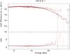 |
Fig. 1 Ho IX X-1: unfolded spectrum. Energy and data-vs-model ratio plot, for only the diskbb model. There are clear residuals above 20 keV. |
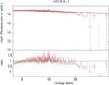 |
Fig. 2 Ho IX X-1: unfolded spectrum. Energy and data-vs.-model ratio plot, for only the power law model. There is a clear curvature in the spectrum that cannot be described by the power law. |
Best fit parameters for the NuSTAR observations.
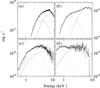 |
Fig. 3 Example, unfolded spectra of two ULXs from our sample and two well known NS-XRBs in the soft state. a) 4U 1705-44, during a soft state. b) Double thermal spectrum from NS-LMXB 4U 1916-05. c) Apparent, dual thermal emission from ULX M81 X-6, at similar temperatures (see Table 2) as 4U 1705-44. d) Similarly shaped spectrum from NGC 4559 X-1. |
The temperature gradient of the accretion curtain will, most likely, differ from the T ~ r-0.75 predicted by the standard thin disk MCD models like diskbb and this deviation will be enhanced further by electron scatterings. To diagnose the impact of this effect on the registered spectra, we also fitted them with the xspec model diskpbb, in which the disk temperature is proportional to r− p and p is a free parameter. We find that the value of p is significantly smaller (on average p ≲ 0.53) than that of a standard thin accretion disk. More interestingly, we find that the diskpbb fits did not require the addition of a power-law tail and yielded the same χ2 values as the diskbb + powerlaw fits; albeit with the notable exception of NGC 5907, which is the only pulsating ULX in our NuSTAR sample. In principle, the diskpbb model could also be used to model the cool thermal emission, detected in the XMM-Newton data, since the inner disk parts may also become inflated due to the high accretion rates (see discussion in Sect. 4). Nevertheless, the addition of an extra free parameter in each thermal component will only add to the degeneracy between different models and will not provide any further insight into the physical parameters (i.e. temperature and size) of the emitting regions. Therefore, the diskpbb model is only used as a diagnostic for the geometry of the accretion curtain, and only for the NuSTAR data where its impact is much more significant; its implications are discussed further in Sect. 4. While we have analysed all available NuSTAR data for our sources, we only tabulate the results for those observations with the largest number of counts and for luminosities closer to the XMM-Newton observations. Nevertheless all NuSTAR observations produced – more or less – similar results to the ones presented here (see observation log in Table 1, for the NuSTAR observations analysed in this work). Best fit values (including the value of p and the temperature of the diskpbb models) for the NuSTAR data are presented in Table 3.
4. Discussion
The use of a double thermal spectrum, with similar temperatures to those observed in the dual thermal spectra of soft-state NS-XRBs, successfully describes the spectra of ULXs in our list and the unusual high-energy roll-over of the ULX spectra can be re-interpreted as the Wien tail of a hot (multicolour) black body component. The similarities between the spectral morphology of ULXs and those of NS-XRBs in the soft state are illustrated in Fig. 3. We have plotted the XMM-Newton spectra of two known NS-XRBs (4U 1916-05 and 4U 1705-44: see Appendix A) along with the spectra of two (non pulsating) ULXs from our sample. Dotted lines correspond to the dual thermal model (in this example it is an absorbed MCD plus black body model) which – in the case of the two NS-XRBs – is used to model emission from the boundary layer and the thin accretion disk. The same configuration is used to model the spectra of the two ULXs (in this example NGC 4559 X-1 and M81 X-6). M81 X-6 is in the BD state and NGC 4559 X-1 in the SUL state. We stress that the unfolded spectra presented in Fig. 3, are model dependent. They are used here in order to illustrate the apparent similarities between the spectral shapes of ULXs and soft-state NS-XRBS and not to extract any quantitative information on the spectral parameters (see also, a similar example plot in Sutton et al. 2013). The suitability of a double thermal model for the spectra of ULXs had been noted by Stobbart et al. (2006); but the model was dismissed, as it was difficult to explain the presence of a secondary thermal component in terms of an accreting black hole. To probe beyond this superficial similarity, we explore the parameter space of the different spectral fits with respect to theoretical expectations, and discuss our findings and their implications below.
Best fit parameters of the MCD plus black body model for the XMM-Newton observations.
More specifically, to investigate the case for (super-Eddington) accretion onto lowly magnetised NSs (e.g. King & Lasota 2016), we applied the diskbb + bbody model that is often used to model NS-XRBs in the soft state. Indeed this model describes well the spectra of the sources in our list. However, the radius inferred from the hot black body fit has a size that is approximately an order of magnitude larger7 than the size of the spreading layer on the surface of the NS (see Table 4). This is not surprising, since at such high accretion rates – and for a low magnetic field NS (as considered in the King & Lasota 2016 model) – the accretion disk will extend well beyond the “spherization” radius (Rsph: Shakura & Sunyaev 1973). The flow will be strongly super-Eddington and the material will, most likely, be ejected away from the surface of NS (e.g. King et al. 2017). In this case the hot thermal component may be the result of emission of the inner disk layers, exposed by the strong outflows. In this case the hot thermal component would correspond to the stripped, inner accretion disk and the soft thermal component, as proposed in the optically thick wind scenario. Indeed, the best fit values for the size of the soft thermal component are in agreement with the Rsph for most of the sources in our list, alluding to the exciting possibility of accreting NSs powering a large fraction of ULXs. However, it is surprising that the dual thermal spectrum would be almost indistinguishable between the BH-ULX and the NS-ULXs, given that in this framework the maximum temperature of the accretion disk should exceed ~ 4 keV in the case of the NSs (perhaps even higher given the very high accretion rates of particular sources). On the other hand, there is still no strictly defined mechanism to account for the hot black body emission for the super-Eddington regime in accreting NS, and a more precise treatment may be able to resolve this apparent discrepancy. The fact still remains that the homogeneous fit parameters hint at the possibility of most (if not all) sources in our sample belonging to one uniform population. It is certainly plausible that this is a population of NS-XRBs instead of BH-XRBs. This implication, becomes even more intriguing when we consider the fact that two of our sources (the pulsators NGC 5907 ULX and NGC 7793 P13) are almost certainly powered by highly magnetised NSs, but – unlike sub-Eddington NS-XRBs – the spectra of pulsating and non-pulsating ULXs are remarkably similar.
The possibility of highly magnetised NSs powering more ULXs in our list becomes even more relevant when we consider that the most reliable and thoroughly established mechanism for sustained super-Eddington accretion episodes is the funneling of material onto the magnetic poles of high-B NSs. Indeed, in a recent publication, Pintore et al. (2017) indicate that since the hard emission from many ULXs can be described by a combination of a hard power law and an exponential cutoff – as expected for the emission of the accretion funnel – this could be considered as an indication in favour of highly magnetised NSs powering a significant fraction of ULXs. However, this claim is problematic, since – in the presence of a high magnetic field – the photons are expected to be concentrated in a narrow beam, most likely following the fan-beam emission diagram. Therefore, as the NS rotates, the emission should be registered in the form of characteristic pulsations.
More importantly, the shape of their pulse profile has a complex shape comprised of two or more characteristic sharp peaks (e.g. Nagel 1981; White et al. 1983; Mészáros 1992; Paul et al. 1996, 1997; Rea et al. 2004; Vasilopoulos et al. 2013, 2014; Koliopanos & Gilfanov 2016). This picture is further complicated by the fact that – most likely – a fraction of the fan-beam emission is scattered by fast electrons at the edge of the accretion column and subsequently beamed towards the surface of the NS (Kaminker et al. 1976; Lyubarskii & Syunyaev 1988; Poutanen et al. 2013) off of which it is reflected, resulting in a secondary “polar” beam, which further complicates the pulse shape (e.g. Trümper et al. 2013; Koliopanos & Vasilopoulos 2017). All but three known ULXs lack any evidence of pulsations and the three pulsating sources (NGC 5907, M82 X-2 and NGC 7793 P13) have very smooth and simple sinusoidal pulse profiles. Therefore, very serious doubts are cast on the interpretation of the ULX spectra as being due to direct emission from the accretion column.
This contradiction appears to be resolved in a new publication by Mushtukov et al. (2017). In this work, the authors demonstrate that highly magnetised NSs, accreting at high mass-accretion rates, can become engulfed in a closed and optically thick envelope (see their Fig. 1). As the primary, beamed emission of the accretion funnel is reprocessed by the optically thick material, the original pulsation information is lost. However, if the latitudinal gradient is sufficiently pronounced – and depending on the viewing angle and inclination of the accretion curtain – the emission may be registered as smooth sinusoidal pulses (this could be the case of the three PULXs). More interestingly, the reprocessed emission is expected to have a multicolour black body (MCB) spectrum with a high temperature (≳ 1.0 keV). The hot MCB component will be accompanied by a cooler (≲ 0.5 keV), thermal component, which originates in a truncated accretion disk. More specifically, the accretion disk is expected to extend uninterrupted, until it reaches the ~ Rmag, where the material follows the magnetic field lines to form the optically thick curtain. In this description the characteristic double thermal spectra of NS-XRBs can coexist with high-B super-Eddington accretion, thus setting NSs as excellent candidates for powering ULXs.
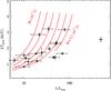 |
Fig. 4 Unabsorbed luminosity (in the 0.5–10 keV range) vs. the temperature (in keV) of the hot multicolour disk component for the XMM-Newton data (Table 2). The (red) solid curves correspond to internal temperature (Tin) of the accretion curtain versus total luminosity, as predicted by Mushtukov et al. (2017; see their Fig. 3). Different curves correspond to different magnetic field strength. From left to right it is 1012, 2 × 10¹², 4 × 10¹², 8 × 10¹², 1.6 × 10¹³ and 3.2 × 10¹³ G. |
In light of these findings, we remodelled the XMM-Newton spectra of the 18 ULXs, using two MCD components. Indeed, the dual MCD model yields marginally better fits than the MCD/black-body fit, in all sources. The best fit values for the temperature and inner radius of the cool MCD component, indicate the presence of a strong magnetic field in all the ULXs in our sample. Namely, their values are consistent with a truncated accretion disk. If we assume that the disk is truncated close to the magnetospheric radius (i.e. to the first approximation Rin = Rmag), we estimate that the intensity of the magnetic field exceeds 1012 G in most sources in our list. More importantly, the temperatures of the hot MCD component and the fit-derived luminosities (see Table 2) occupy the same parameter space, as predicted by Mushtukov et al. (2017: their Fig. 3, and also Fig. 4 in this work). Namely, the best-fit values for kThot appear to follow the theoretical curves predicted in Mushtukov et al. (2017) and as a general trend, sources with stronger magnetic fields are more luminous (see Fig. 5) and have a hotter accretion curtain. The observed correlation between the magnetic field strength and the source luminosity is in agreement with the predictions of Mushtukov et al. (2015a), where the accretion luminosity of magnetised neutron stars, in the super-critical regime, is discussed.
Following this scheme, we also place NGC 5907 ULX in the magnetar regime (B ~ 1.8 × 10¹⁴ G) which is in agreement with the findings of Israel et al. (2017). As Israel et al. also point out, such a high value of the magnetic field is puzzling8, since the source should be repeatedly entering the propeller regime (Illarionov & Sunyaev 1975; Stella et al. 1986). However, we must underline the fact that the magnetic field values presented in this work are estimated based on the crude assumption that the Rmag is equal to the truncation radius of a thin Shakura-Sunyaev disk accreting onto a bipolar magnetic field. As such, the derived values should be treated as indications of a strongly magnetised accretor, but not considered at face value. A more realistic treatment of specific sources could yield B-field values of up to a factor of 5–6 times lower. For instance, if we re-estimate the magnetic values using the latest considerations of Chashkina et al. (2017) – where it is shown that in the radiation-pressure-dominated regime, the size of the magnetosphere is independent of the mass accretion rate (see their Eqs. (39), (41) and (61)) – we end up with a value of B ~ 3.5 × 10¹³ G for NGC 5907 ULX and a factor of ~ 30−470% lower magnetic field values for the other sources in our list. Nevertheless, the main outcome of our analysis remains. The best-fit parameters are consistent with our underlying assumption of a high magnetic field, which reinforces the plausibility of this scenario. A similar scenario – in which (non pulsating) ULXs are interpreted as high-B NSs in a supercritical propeller stage – is also proposed by Ekşi (2017) in a study that was submitted for publication in MNRAS, during the refereeing process of this work.
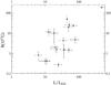 |
Fig. 5 Magnetic field strength vs. Luminosity for the dual MCD model. All values are taken from Table 2 (Cols. 6 and 8). |
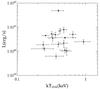 |
Fig. 6 Luminosity vs. disk temperature for the dual MCD model. All values are taken from Table 2 (Cols. 3 and 6). |
An additional implication of the high magnetic fields is the requirement that these sources are very young. Depending on the initial value of the magnetic field (which in this scenario should be at magnetar levels), the initial spin period, and the mass accretion rate, these sources are most likely younger than ~ 5 × 10⁶ yr, if we assume that they currently have a magnetic field of the order of 1012 G (e.g. Ghosh & Lamb 1979; Zhang & Kojima 2006; Pan et al. 2016). Indications in favour of a relatively young age (of the order of ~10 Myr) can be maintained for sources HoII X-1, HoIX X-1, IC342 X-1, M81 X-6, NGC 1313 X-2, NGC 253 XMM2, NGC 253 ULX2, NGC 4559, NGC 4736 and NGC 5204, which are associated with young stellar environments and star forming regions (Soria et al. 2005; Liu et al. 2007; Grisé et al. 2008; Berghea et al. 2008, 2010; Grisé et al. 2011; Berghea et al. 2013). Furthermore, sources HoII X-1, HoIX X-1, IC342 X-1, M81 X-6, NGC 1313 X-2 and NGC 5204 have optical counterparts indicating that they are very young objects (Zampieri et al. 2004; Kaaret et al. 2004; Ramsey et al. 2006), while the nebula of IC 342 X-1 and HoIX X-1 indicate activity of less than ~1 Myr (Pakull & Mirioni 2002; Kaaret et al. 2004; Abolmasov et al. 2007; Feng & Kaaret 2008; Cseh et al. 2012). However, estimation of the stellar companion’s age based on the optical counterpart can be hindered by the fact that its emission may originate in the (irradiated) outer accretion disk, rather than the photosphere of the donor star (e.g. Grisé et al. 2012; Tao et al. 2012a,b). Furthermore, the magnetic field values inferred from the spectral fitting of some of our sources would require even younger ages than those derived from observations – that is, for B ≳ 1013 G and assuming standard magnetic field decay (e.g. Frank et al. 2002; Zhang & Kojima 2006). Therefore, investigation for further indications of the presence of magnetic field in ULXs and more accurate estimation of the magnetic field strength is required to explore this intriguing scenario.
If the “cool” MCD component, indeed originated in a truncated accretion disk, we would expect a positive correlation between the disk temperature (Tdisk) and the bolometric luminosity (L) as argued by Miller et al. (2013). In Fig. 6 we have plotted Rdisk versus Tdisk, however, since the accretion disk is expected to become truncated at different values of Rdisk (which in our scheme correspond to different B-field strength and mass accretion rates of different sources), there is a large scatter in the derived values and an accurate estimation of the L ~ T relation cannot be attempted. Regarding our choice to model the cool thermal emission using a thin disk model, we must note that while in all sources analysed in this work the Rmag is larger than Rsph (for any plausible value of fcol) and therefore the accretion disk could be assumed to remain thin, the Rmag values are only nominally larger than Rsph and – more importantly – the fit-inferred luminosities of the disk component are super-Eddington, suggesting that the disk will most likely be geometrically thick. In this case we would expect that the advection will perturb the thin MCD spectrum which we have used to model the cool thermal component. Nevertheless, this will not introduce any significant qualitative difference in our results (see e.g. Straub et al. 2013; and also discussion in Mushtukov et al. 2017) and therefore – as with the hot thermal component – the diskbb model is sufficient for the purposes of this work. Another potential issue of the geometrically thick disk is the expected emergence of outflows due to the radiation pressure, which may put the stability of this mechanism into question. However, in the presence of strong magnetic fields, the accreting, optically thick material will remain bound, even for luminosities of the order of ~ 1040 erg/s (Mushtukov et al. 2017; Chashkina et al. 2017).
We also note that the numerically estimated curves in Fig. 3 of Mushtukov et al., refer to the internal temperature (Tin: is the temperature of the inner boundary of the emission curtain, which faces the NS) of the geometrically thick accretion envelope. In the optically thick regime, Tin is related to Tout (which corresponds to the observed Thot) as,  (6)Therefore, the values of Thot presented in Fig. 4 should be multiplied by a factor of ≈ 1.8−2.1 (corresponding to an optically thick corona, i.e. τ ≈ 10−20) in order to represent the internal temperature (Tin). However, as stated in Sect. 3, in our temperature estimations we have ignored the spectral hardening which would have produced colour-corrected temperatures given by Tcor = Thot/fcol, with fcol ranging between 1.5 and 2.1. This notable consistency between the colour correction factor and the relation between internal and external temperature in an optically thick accretion envelope further reinforces its plausibility, and with it, our confidence in the observational verification of this new scheme proposed by Mushtukov et al. (2017).
These intriguing findings are also supported by the NuSTAR observations. Indeed, analysis of the NuSTAR data confirms the presence of the <10 keV roll over, observed in the XMM-Newton data (see e.g. Fig. 2). More importantly, when the spectral curvature is modelled as hot MCB emission, the temperatures of the diskbb component in the NuSTAR data are in agreement with the XMM-Newton observations, particularly in those sources that were observed at similar luminosity. The presence of a thermal-like component in the NuSTAR spectra of ULXs has also been noted for sources Circinus ULX5 (Walton et al. 2013) and NGC 5204 X-1 (Mukherjee et al. 2015), further supporting the case for emission from hot, optically thick material.
Indications for the presence of optically thick material at the boundary of the magnetosphere can also be found in sources that lie below the Eddington limit. Several X-ray pulsars (in the sub-Eddington regime) exhibit a characteristic spectral “soft excess”, which is well described by a black body distribution at a temperature of ~0.1–0.2 keV (e.g. Hickox et al. 2004, and references therein). This emission has been attributed to reprocessing of hard X-rays by optically thick material in the vicinity of the magnetosphere. The size of the reprocessing region is considerably larger than the inner edge of a standard accretion disk and it is argued that it may partially cover the primary hard emission from the accretion column (e.g. Zurita Heras et al. 2006; La Palombara & Mereghetti 2006; Reig et al. 2009; Sidoli et al. 2015). It is plausible that the predictions of Mushtukov et al. (2017) are – in essence – an expansion of these arguments to the super-Eddington regime, where the optically thick material engulfs the entire magnetosphere, obfuscating most (or all) of the primary hard emission. The resulting accretion envelope has a temperature that is an order of magnitude higher than that of the soft excess in the sub-Eddington sources.
The NuSTAR data also reveal the presence of a weak power law above ~ 15 keV. The hard emission, which is often present in the spectra of NS-XRBs in the soft state (e.g. Barret 2001; Done et al. 2007; Lin et al. 2009, and references therein), has also been noted by Walton et al. (2014), Walton et al. (2015), and Fürst et al. (2017) in NuSTAR data of Ho IX X-1, Ho II X-1, and NGC 5907 ULX, respectively. The thermal emission of the accretion curtain may be modified by IC scattering from a photoionised atmosphere, analogous to an accretion disk corona (e.g. Sunyaev & Titarchuk 1980; Haardt & Maraschi 1993). The presence of this highly ionised plasma is also supported by the detection of emission-like features in some of the observations in our list (see Sect. 3). We note that the presence of similar, broad-emission-like features centred at ~ 1 keV have also been detected in the spectra of “nominal” X-ray pulsars at lower accretion rates (e.g. Ramsay et al. 2002; Sidoli et al. 2015; La Palombara et al. 2016), which also exhibit the soft excess.
We must also highlight the possibility that the apparent power-law tail may in fact be an artifact, resulting from modelling the MCB emission of the quasi-spherical accretion curtain with a MCD model. In Sect. 3, it was noted that when we model the hot thermal component with a MCB model where Thot is proportional to r− p and p is left to vary freely, the NuSTAR spectra can be successfully fitted without the requirement for the hard tail. More specifically, in all cases, the value of p is less than ~0.58, which – in the context of accretion disks – points to an “inflated”, advective, slim disk (e.g. Kubota & Makishima 2004, and references therein). In this case, it is fairly plausible that the radically different geometry of the accretion curtain will cause a significant deviation from the temperature gradient of T ~ r-0.75 assumed by the standard MCD model used in our fits, resulting in an underestimation of the hard emission, which appears as an excess above ~ 15 keV.
The hypothesis of an “obscured”, highly magnetised NS as the central engine in ULXs may also resolve the contradiction regarding the only known (to this date) detection of a relativistic jet in a ULX, in Ho II X-1 (Cseh et al. 2015). While collimated jets are often detected in BH-XRBs and AGN, they are only present during the low-accretion, non-thermal hard state. In the case of Ho II X-1, though, the collimated jet is detected in a high accretion state, during which the spectrum is dominated by thermal emission, which is in stark contrast to the BH-XRB/jet paradigm. This contradiction is resolved when we consider a high-B NS as the accretor, which – for sufficiently high values of the magnetic field – can power collimated relativistic jets at high accretion rates (Parfrey et al. 2016, 2017). However, in this framework the presence of the jet is also contingent upon the NS spin period. Only a limited set of parameters would yield a powerful jet in the high accretion-rate regime, which may explain the lack of a jet in most known ULXs. It is also certainly plausible that the non-detection of radio jets may be the result of a lack of sensitivity, since the expected flux would most likely lie in the few μ Jy range or less. Given the above discussion and the bulk of theoretical expectations, strong outflows should be expected for any type of accretor (i.e. BH, highly or lowly magnetised NS). The more pertinent question, then, would be whether the soft thermal component originates in a hot optically thick wind component, close to the accretor or the truncated accretion disk. Therefore, given the recent considerations regarding the different candidates for the ULX accretors, it is important that the evolution of the Lsoft ~ Tin relation for specific sources is revisited.
The “universal”, power-law-shaped luminosity function of ULXs and HMXBs (e.g. Gilfanov et al. 2004; Swartz et al. 2004; Mineo et al. 2012) may also be interpreted as favouring NS-powered ULXs. More specifically, the smooth shape of the HMXB luminosity function up to log L ~ 40.5 strongly implies that ULXs are composed of ordinary HXMBs with stellar-mass accretors. Since most HMXBs are powered by NSs (e.g. Liu et al. 2006; Belczynski & Ziolkowski 2009) and also most ULXs are found in star-forming regions (e.g. Feng & Soria 2011, and references therein) that favour the evolution of NS-HMXBs, it is reasonable to postulate that most ULXs are indeed NS-XRBs. It is also of great interest to investigate if there are fundamentally different characteristics between ULXs and sources that lie above the ~ 1040 erg/s break in the luminosity function (Mineo et al. 2012). Indeed the two brightest HLXs – M82 X-1 and ESO 243-49 HLX-1 – do not feature the spectral cutoff of ULXs (e.g. Dewangan et al. 2006; Farrell et al. 2009) and also appear to transition between the empirical BH-XRB accretion states (e.g. Godet et al. 2009; Feng & Kaaret 2010; although Brightman et al. 2016, recently indicated that M82 X-1, during episodes of high accretion, can be modelled as a stellar-mass BH, accreting at super-Eddington rates). The differing aspects between sources above and below the luminosity break indicate a different type of accretor between HLXs and ULXs. Within the scheme discussed in this work, this could mean that while most ULXs have NS accretors, HLXs harbour either supercritically accreting stellar-BHs or sub-Eddington accreting IMBHs. Nevertheless, given the very small sample of HLX sources, such hypotheses remain strictly in the realm of speculation.
5. Conclusion
We have presented an alternative interpretation of the X-ray spectra of eighteen well-known ULXs, which provides physically meaningful spectral parameters. More specifically, from the analysis of the XMM-Newton and NuSTAR spectra, we note that the curvature above ~5 keV – found in the spectra of most ULXs – is consistent with the Wien tail of thermal emission in the >1 keV range. Furthermore the high-quality XMM-Newton spectra confirm the presence of a secondary, cooler thermal component. These findings are in agreement with the analysis presented in previous works (e.g. Walton et al. 2014, 2015; Luangtip et al. 2016). However, in contrast to the currently accepted paradigm, we propose that the dual thermal spectrum may be the result of accretion onto a highly magnetised NS, as predicted in recent theoretical models (Mushtukov et al. 2017) in which the hot thermal component originates in an optically thick envelope that engulfs the entire NS at the boundary of the magnetosphere, and the soft thermal component originates in an accretion disk that becomes truncated at approximately the magnetospheric radius. We claim that this finding offers an additional and compelling argument in favour of neutron stars as more suitable candidates for powering ULXs, as has been recently suggested (King & Lasota 2016; King et al. 2017). In light of this interpretation, the ultraluminous state classification put forward by Sutton et al. (2013) can be re-interpreted in terms of different temperatures and relative flux contribution of the two thermal components, which result in the different spectral morphologies.
Nevertheless, we stress that there is considerable degeneracy between different models that can fit the spectra equally well, and so far there are no observational features, such as cyclotron lines or transitions to the propeller regime (e.g. Pringle & Rees 1972; Lamb et al. 1973; Illarionov & Sunyaev 1975), that will conclusively favour this hypothesis over other comprehensive and equally plausible interpretations (i.e. optically thick outflows from critically accreting black holes). Furthermore, the presence of strong outflows is also expected in the case of accreting high field NSs, which may account for the soft thermal emission in the NS scenario as well. Given the encouraging results of this work, further examination of this scenario is warranted. To this end, the fractional variability of ULXs (which is addressed by the BH super-Eddington wind model) should be reviewed in the context of the highly magnetised NS model, and the possibility of aperiodic flux variation due to the rotating accretion curtain must be explored further. Moreover, deeper broadband observations that will also allow precise phase resolved spectroscopy of the pulsating sources, as well as long-term monitoring – in sources for which this is feasible – are necessary in order to further probe this newly emerging paradigm.
XMM-Newton CCF Release Note: XMM-CCF-REL-332.
See XMM-Newton Users Handbook Sect. 3.2.1.1, http://xmm-tools.cosmos.esa.int/external/xmm_user_support/documentation/uhb/onaxisxraypsf.html
When part of the psf lies in a chip gap, effective exposure and encircled energy fraction may be affected.
Or inner radius in the case of an accretion disk.
With the exception of NGC 55 ULX, which does show dips in its light curve (Stobbart et al. 2004). However, due to its likely supercritical accretion rates, the dips are not as constraining, for its inclination, as in typical XRBs.
The boundary layer is expected to be a few km in size (Lin et al. 2009; and Table A.1 in this work).
In Israel et al. (2017) a multi-pole component is proposed as a resolution.
Acknowledgments
The authors would like to thank the anonymous referee whose contribution significantly improved our manuscript. Also, F.K., O.G., N.W. and D.B. acknowledge support from the CNES. F.K. warmly thanks Apostolos Mastichiadis and Maria Petropoulou for comments and stimulating discussion.
References
- Abolmasov, P., Fabrika, S., Sholukhova, O., & Afanasiev, V. 2007, Astrophysical Bulletin, 62, 36 [NASA ADS] [CrossRef] [Google Scholar]
- Arnaud, K. A. 1996, in Astronomical Data Analysis Software and Systems V, eds. G. H. Jacoby, & J. Barnes, ASP Conf. Ser., 101, 17 [Google Scholar]
- Bachetti, M. 2016, Astron. Nachr., 337, 349 [NASA ADS] [CrossRef] [Google Scholar]
- Bachetti, M., Rana, V., Walton, D. J., et al. 2013, ApJ, 778, 163 [NASA ADS] [CrossRef] [Google Scholar]
- Bachetti, M., Harrison, F. A., Walton, D. J., et al. 2014, Nature, 514, 202 [NASA ADS] [CrossRef] [Google Scholar]
- Barret, D. 2001, Adv. Space Res., 28, 307 [NASA ADS] [CrossRef] [Google Scholar]
- Basko, M. M. 1980, A&A, 87, 330 [NASA ADS] [Google Scholar]
- Basko, M. M., & Sunyaev, R. A. 1975, A&A, 42, 311 [NASA ADS] [Google Scholar]
- Basko, M. M., & Sunyaev, R. A. 1976, MNRAS, 175, 395 [NASA ADS] [CrossRef] [Google Scholar]
- Becker, P. A., & Wolff, M. T. 2007, ApJ, 654, 435 [NASA ADS] [CrossRef] [Google Scholar]
- Begelman, M. C., & Chiueh, T. 1988, ApJ, 332, 872 [NASA ADS] [CrossRef] [Google Scholar]
- Belczynski, K., & Ziolkowski, J. 2009, ApJ, 707, 870 [NASA ADS] [CrossRef] [Google Scholar]
- Belmont, R., Malzac, J., & Marcowith, A. 2008, A&A, 491, 617 [NASA ADS] [CrossRef] [EDP Sciences] [Google Scholar]
- Berghea, C. T., Weaver, K. A., Colbert, E. J. M., & Roberts, T. P. 2008, ApJ, 687, 471 [NASA ADS] [CrossRef] [Google Scholar]
- Berghea, C. T., Dudik, R. P., Weaver, K. A., & Kallman, T. R. 2010, ApJ, 708, 354 [NASA ADS] [CrossRef] [Google Scholar]
- Berghea, C. T., Dudik, R. P., Tincher, J., & Winter, L. M. 2013, ApJ, 776, 100 [NASA ADS] [CrossRef] [Google Scholar]
- Boirin, L., & Parmar, A. N. 2003, A&A, 407, 1079 [NASA ADS] [CrossRef] [EDP Sciences] [Google Scholar]
- Boirin, L., Parmar, A. N., Barret, D., Paltani, S., & Grindlay, J. E. 2004, A&A, 418, 1061 [NASA ADS] [CrossRef] [EDP Sciences] [Google Scholar]
- Brightman, M., Harrison, F. A., Barret, D., et al. 2016, ApJ, 829, 28 [NASA ADS] [CrossRef] [Google Scholar]
- Burnard, D. J., Arons, J., & Klein, R. I. 1991, ApJ, 367, 575 [CrossRef] [Google Scholar]
- Caballero, I., & Wilms, J. 2012, Mem. Soc. Astron. It., 83, 230 [NASA ADS] [Google Scholar]
- Canuto, V., Lodenquai, J., & Ruderman, M. 1971, Phys. Rev. D, 3, 2303 [NASA ADS] [CrossRef] [Google Scholar]
- Chashkina, A., Abolmasov, P., & Poutanen, J. 2017, MNRAS, 470, 2799 [NASA ADS] [CrossRef] [Google Scholar]
- Colbert, E. J. M., & Mushotzky, R. F. 1999, ApJ, 519, 89 [NASA ADS] [CrossRef] [Google Scholar]
- Coppi, P. S. 1999, in High Energy Processes in Accreting Black Holes, eds. J. Poutanen, & R. Svensson, ASP Conf. Ser., 161, 375 [Google Scholar]
- Coppi, P. S., & Blandford, R. D. 1990, MNRAS, 245, 453 [NASA ADS] [Google Scholar]
- Cseh, D., Corbel, S., Kaaret, P., et al. 2012, ApJ, 749, 17 [NASA ADS] [CrossRef] [Google Scholar]
- Cseh, D., Miller-Jones, J. C. A., Jonker, P. G., et al. 2015, MNRAS, 452, 24 [NASA ADS] [CrossRef] [Google Scholar]
- Dewangan, G. C., Titarchuk, L., & Griffiths, R. E. 2006, ApJ, 637, L21 [NASA ADS] [CrossRef] [Google Scholar]
- DíazTrigo, M., Parmar, A. N., Boirin, L., Méndez, M., & Kaastra, J. S. 2006, A&A, 445, 179 [NASA ADS] [CrossRef] [EDP Sciences] [Google Scholar]
- Dickey, J. M., & Lockman, F. J. 1990, ARA&A, 28, 215 [NASA ADS] [CrossRef] [MathSciNet] [Google Scholar]
- Done, C., Gierliński, M., & Kubota, A. 2007, A&ARv, 15, 1 [NASA ADS] [CrossRef] [EDP Sciences] [Google Scholar]
- Ebisawa, K., Day, C. S. R., Kallman, T. R., et al. 1996, PASJ, 48, 425 [NASA ADS] [Google Scholar]
- Ekşi, K. Y. 2017, arXiv e-prints [arXiv:1708.04502] [Google Scholar]
- Fabrika, S., Ueda, Y., Vinokurov, A., Sholukhova, O., & Shidatsu, M. 2015, Nat. Phys., 11, 551 [NASA ADS] [CrossRef] [Google Scholar]
- Farrell, S. A., Webb, N. A., Barret, D., Godet, O., & Rodrigues, J. M. 2009, Nature, 460, 73 [NASA ADS] [CrossRef] [PubMed] [Google Scholar]
- Feng, H., & Kaaret, P. 2008, ApJ, 675, 1067 [NASA ADS] [CrossRef] [Google Scholar]
- Feng, H., & Kaaret, P. 2010, ApJ, 712, L169 [NASA ADS] [CrossRef] [Google Scholar]
- Feng, H., & Soria, R. 2011, New Astron. Rev., 55, 166 [NASA ADS] [CrossRef] [Google Scholar]
- Feng, H., Tao, L., Kaaret, P., & Grisé, F. 2016, ApJ, 831, 117 [NASA ADS] [CrossRef] [Google Scholar]
- Frank, J., King, A., & Raine, D. J. 2002, Accretion Power in Astrophysics: third edition (Cambridge, UK: Cambridge University Press) [Google Scholar]
- Frankel, N. E., Hines, K. C., & Dewar, R. L. 1979, Phys. Rev. A, 20, 2120 [NASA ADS] [CrossRef] [Google Scholar]
- Fürst, F., Walton, D. J., Harrison, F. A., et al. 2016, ApJ, 831, L14 [NASA ADS] [CrossRef] [Google Scholar]
- Fürst, F., Walton, D. J., Stern, D., et al. 2017, ApJ, 834, 77 [NASA ADS] [CrossRef] [Google Scholar]
- Gallo, E., Fender, R. P., & Pooley, G. G. 2003, MNRAS, 344, 60 [NASA ADS] [CrossRef] [Google Scholar]
- Gao, Y., Wang, Q. D., Appleton, P. N., & Lucas, R. A. 2003, ApJ, 596, L171 [NASA ADS] [CrossRef] [Google Scholar]
- Ghosh, P., & Lamb, F. K. 1979, ApJ, 234, 296 [NASA ADS] [CrossRef] [Google Scholar]
- Gilfanov, M. 2010, in Lect. Notes Phys., ed. T. Belloni (Berlin: Springer Verlag), 794, 17 [Google Scholar]
- Gilfanov, M., Grimm, H.-J., & Sunyaev, R. 2004, Nucl. Phys. B Proc. Suppl., 132, 369 [NASA ADS] [CrossRef] [Google Scholar]
- Gladstone, J. C., Roberts, T. P., & Done, C. 2009, MNRAS, 397, 1836 [NASA ADS] [CrossRef] [Google Scholar]
- Gnedin, Y. N., & Sunyaev, R. A. 1973, A&A, 25, 233 [NASA ADS] [Google Scholar]
- Godet, O., Barret, D., Webb, N. A., Farrell, S. A., & Gehrels, N. 2009, ApJ, 705, L109 [NASA ADS] [CrossRef] [Google Scholar]
- Gould, R. J. 1975, ApJ, 196, 689 [NASA ADS] [CrossRef] [Google Scholar]
- Grisé, F., Pakull, M. W., Soria, R., et al. 2008, A&A, 486, 151 [NASA ADS] [CrossRef] [EDP Sciences] [Google Scholar]
- Grisé, F., Kaaret, P., Feng, H., Kajava, J. J. E., & Farrell, S. A. 2010, ApJ, 724, L148 [NASA ADS] [CrossRef] [Google Scholar]
- Grisé, F., Kaaret, P., Pakull, M. W., & Motch, C. 2011, ApJ, 734, 23 [NASA ADS] [CrossRef] [Google Scholar]
- Grisé, F., Kaaret, P., Corbel, S., et al. 2012, ApJ, 745, 123 [NASA ADS] [CrossRef] [Google Scholar]
- Haardt, F., & Maraschi, L. 1993, ApJ, 413, 507 [NASA ADS] [CrossRef] [MathSciNet] [Google Scholar]
- Hickox, R. C., Narayan, R., & Kallman, T. R. 2004, ApJ, 614, 881 [NASA ADS] [CrossRef] [Google Scholar]
- Illarionov, A. F., & Sunyaev, R. A. 1975, A&A, 39, 185 [NASA ADS] [Google Scholar]
- Ingram, A., & van der Klis, M. 2013, MNRAS, 434, 1476 [NASA ADS] [CrossRef] [Google Scholar]
- Israel, G. L., Belfiore, A., Stella, L., et al. 2017, Science, 355, 817 [NASA ADS] [CrossRef] [Google Scholar]
- Kaaret, P., Prestwich, A. H., Zezas, A., et al. 2001, MNRAS, 321, L29 [Google Scholar]
- Kaaret, P., Ward, M. J., & Zezas, A. 2004, MNRAS, 351, L83 [NASA ADS] [CrossRef] [Google Scholar]
- Kaaret, P., Feng, H., & Roberts, T. P. 2017, ARA&A, 55, 303 [Google Scholar]
- Kajava, J. J. E., & Poutanen, J. 2009, MNRAS, 398, 1450 [NASA ADS] [CrossRef] [Google Scholar]
- Kajava, J. J. E., Poutanen, J., Farrell, S. A., Grisé, F., & Kaaret, P. 2012, MNRAS, 422, 990 [NASA ADS] [CrossRef] [Google Scholar]
- Kaminker, A. D., Fedorenko, V. N., & Tsygan, A. I. 1976, Sov. Astron., 20, 436 [NASA ADS] [Google Scholar]
- King, A. R. 2009, MNRAS, 393, L41 [NASA ADS] [Google Scholar]
- King, A., & Lasota, J.-P. 2016, MNRAS, 458, L10 [Google Scholar]
- King, A. R., & Pounds, K. A. 2003, MNRAS, 345, 657 [NASA ADS] [CrossRef] [Google Scholar]
- King, A. R., Davies, M. B., Ward, M. J., Fabbiano, G., & Elvis, M. 2001, ApJ, 552, L109 [NASA ADS] [CrossRef] [Google Scholar]
- King, A., Lasota, J.-P., & Kluźniak, W. 2017, MNRAS, 468, L59 [NASA ADS] [CrossRef] [Google Scholar]
- Kolehmainen, M., Done, C., & Díaz Trigo, M. 2014, MNRAS, 437, 316 [NASA ADS] [CrossRef] [Google Scholar]
- Koliopanos, F., & Gilfanov, M. 2016, MNRAS, 456, 3535 [NASA ADS] [CrossRef] [Google Scholar]
- Koliopanos, F., & Vasilopoulos, G. 2017, A&A, submitted [Google Scholar]
- Kubota, A., & Makishima, K. 2004, ApJ, 601, 428 [NASA ADS] [CrossRef] [Google Scholar]
- La Palombara, N., & Mereghetti, S. 2006, A&A, 455, 283 [NASA ADS] [CrossRef] [EDP Sciences] [Google Scholar]
- La Palombara, N., Sidoli, L., Pintore, F., et al. 2016, MNRAS, 458, L74 [NASA ADS] [Google Scholar]
- Lai, D. 2014, in Eur. Phys. J. Web Conf., 64, 01001 [Google Scholar]
- Lamb, F. K., Pethick, C. J., & Pines, D. 1973, ApJ, 184, 271 [NASA ADS] [CrossRef] [Google Scholar]
- Lapidus, I. I., Syunyaev, R. A., & Titarchuk, L. G. 1986, Sov. Astron. Lett., 12, 383 [NASA ADS] [Google Scholar]
- Lin, D., Remillard, R. A., & Homan, J. 2007, ApJ, 667, 1073 [NASA ADS] [CrossRef] [Google Scholar]
- Lin, D., Remillard, R. A., & Homan, J. 2009, ApJ, 696, 1257 [NASA ADS] [CrossRef] [Google Scholar]
- Liu, Q. Z., van Paradijs, J., & van den Heuvel, E. P. J. 2006, A&A, 455, 1165 [NASA ADS] [CrossRef] [EDP Sciences] [Google Scholar]
- Liu, J.-F., Bregman, J., Miller, J., & Kaaret, P. 2007, ApJ, 661, 165 [NASA ADS] [CrossRef] [Google Scholar]
- Lodenquai, J., Canuto, V., Ruderman, M., & Tsuruta, S. 1974, ApJ, 190, 141 [NASA ADS] [CrossRef] [Google Scholar]
- London, R. A., Taam, R. E., & Howard, W. M. 1986, ApJ, 306, 170 [Google Scholar]
- Luangtip, W., Roberts, T. P., & Done, C. 2016, MNRAS, 460, 4417 [NASA ADS] [CrossRef] [Google Scholar]
- Lyubarskii, Y. E., & Syunyaev, R. A. 1988, Sov. Astron. Lett., 14, 390 [NASA ADS] [Google Scholar]
- Makishima, K., Kubota, A., Mizuno, T., et al. 2000, ApJ, 535, 632 [NASA ADS] [CrossRef] [Google Scholar]
- Malzac, J., & Belmont, R. 2009, MNRAS, 392, 570 [NASA ADS] [CrossRef] [Google Scholar]
- Mészáros, P. 1992, High-energy radiation from magnetized neutron stars (University of Chicago Press) [Google Scholar]
- Meszaros, P., & Nagel, W. 1985, ApJ, 299, 138 [CrossRef] [Google Scholar]
- Middleton, M. J., Sutton, A. D., & Roberts, T. P. 2011, MNRAS, 417, 464 [NASA ADS] [CrossRef] [Google Scholar]
- Middleton, M. J., Walton, D. J., Roberts, T. P., & Heil, L. 2014, MNRAS, 438, L51 [NASA ADS] [CrossRef] [Google Scholar]
- Middleton, M. J., Heil, L., Pintore, F., Walton, D. J., & Roberts, T. P. 2015a, MNRAS, 447, 3243 [NASA ADS] [CrossRef] [Google Scholar]
- Middleton, M. J., Walton, D. J., Fabian, A., et al. 2015b, MNRAS, 454, 3134 [NASA ADS] [CrossRef] [Google Scholar]
- Miller, J. M., Fabbiano, G., Miller, M. C., & Fabian, A. C. 2003, ApJ, 585, L37 [NASA ADS] [CrossRef] [Google Scholar]
- Miller, J. M., Walton, D. J., King, A. L., et al. 2013, ApJ, 776, L36 [NASA ADS] [CrossRef] [Google Scholar]
- Mineo, S., Gilfanov, M., & Sunyaev, R. 2012, MNRAS, 419, 2095 [NASA ADS] [CrossRef] [Google Scholar]
- Mitsuda, K., Inoue, H., Koyama, K., et al. 1984, PASJ, 36, 741 [NASA ADS] [Google Scholar]
- Mitsuda, K., Inoue, H., Nakamura, N., & Tanaka, Y. 1989, PASJ, 41, 97 [NASA ADS] [Google Scholar]
- Mukherjee, E. S., Walton, D. J., Bachetti, M., et al. 2015, ApJ, 808, 64 [NASA ADS] [CrossRef] [Google Scholar]
- Muno, M. P., Remillard, R. A., & Chakrabarty, D. 2002, ApJ, 568, L35 [NASA ADS] [CrossRef] [Google Scholar]
- Mushtukov, A. A., Suleimanov, V. F., Tsygankov, S. S., & Poutanen, J. 2015a, MNRAS, 454, 2539 [Google Scholar]
- Mushtukov, A. A., Suleimanov, V. F., Tsygankov, S. S., & Poutanen, J. 2015b, MNRAS, 447, 1847 [NASA ADS] [CrossRef] [Google Scholar]
- Mushtukov, A. A., Suleimanov, V. F., Tsygankov, S. S., & Ingram, A. 2017, MNRAS, 467, 1202 [NASA ADS] [Google Scholar]
- Nagase, F., Corbet, R. H. D., Day, C. S. R., et al. 1992, ApJ, 396, 147 [NASA ADS] [CrossRef] [Google Scholar]
- Nagel, W. 1981, ApJ, 251, 288 [NASA ADS] [CrossRef] [Google Scholar]
- Narayan, R. 2005, Ap&SS, 300, 177 [NASA ADS] [CrossRef] [Google Scholar]
- Ng, C., Díaz Trigo, M., Cadolle Bel, M., & Migliari, S. 2010, A&A, 522, A96 [NASA ADS] [CrossRef] [EDP Sciences] [Google Scholar]
- Pakull, M. W., & Mirioni, L. 2002, ArXiv e-print [arXiv:astro-ph/0202488] [Google Scholar]
- Pakull, M. W., & Mirioni, L. 2003, in Rev. Mex. Astron. Astrofis. Conf. Ser., 15, eds. J. Arthur, & W. J. Henney, 197 [Google Scholar]
- Pan, Y. Y., Song, L. M., Zhang, C. M., & Tong, H. 2016, MNRAS, 461, 2 [NASA ADS] [CrossRef] [Google Scholar]
- Parfrey, K., Spitkovsky, A., & Beloborodov, A. M. 2016, ApJ, 822, 33 [NASA ADS] [CrossRef] [Google Scholar]
- Parfrey, K., Spitkovsky, A., & Beloborodov, A. M. 2017, MNRAS, 469, 3656 [NASA ADS] [CrossRef] [Google Scholar]
- Paul, B., Agrawal, P. C., Rao, A. R., & Manchanda, R. K. 1996, BASI, 24, 729 [Google Scholar]
- Paul, B., Agrawal, P. C., Rao, A. R., & Manchanda, R. K. 1997, A&A, 319, 507 [NASA ADS] [Google Scholar]
- Pinto, C., Middleton, M. J., & Fabian, A. C. 2016, Nature, 533, 64 [NASA ADS] [CrossRef] [Google Scholar]
- Pinto, C., Alston, W., Soria, R., et al. 2017, MNRAS, 468, 2865 [NASA ADS] [CrossRef] [Google Scholar]
- Pintore, F., & Zampieri, L. 2012, MNRAS, 420, 1107 [NASA ADS] [CrossRef] [Google Scholar]
- Pintore, F., Zampieri, L., Wolter, A., & Belloni, T. 2014, MNRAS, 439, 3461 [NASA ADS] [CrossRef] [Google Scholar]
- Pintore, F., Zampieri, L., Stella, L., et al. 2017, ApJ, 836, 113 [Google Scholar]
- Poutanen, J., Lipunova, G., Fabrika, S., Butkevich, A. G., & Abolmasov, P. 2007, MNRAS, 377, 1187 [NASA ADS] [CrossRef] [Google Scholar]
- Poutanen, J., Mushtukov, A. A., Suleimanov, V. F., et al. 2013, ApJ, 777, 115 [NASA ADS] [CrossRef] [Google Scholar]
- Pringle, J. E., & Rees, M. J. 1972, A&A, 21, 1 [NASA ADS] [Google Scholar]
- Ramsay, G., Zane, S., Jimenez-Garate, M. A., den Herder, J.-W., & Hailey, C. J. 2002, MNRAS, 337, 1185 [NASA ADS] [CrossRef] [Google Scholar]
- Ramsey, C. J., Williams, R. M., Gruendl, R. A., et al. 2006, ApJ, 641, 241 [NASA ADS] [CrossRef] [Google Scholar]
- Rana, V., Harrison, F. A., Bachetti, M., et al. 2015, ApJ, 799, 121 [NASA ADS] [CrossRef] [Google Scholar]
- Rea, N., Israel, G. L., Di Salvo, T., Burderi, L., & Cocozza, G. 2004, A&A, 421, 235 [NASA ADS] [CrossRef] [EDP Sciences] [Google Scholar]
- Reig, P., Torrejón, J. M., Negueruela, I., et al. 2009, A&A, 494, 1073 [NASA ADS] [CrossRef] [EDP Sciences] [Google Scholar]
- Remillard, R. A., & McClintock, J. E. 2006, ARA&A, 44, 49 [NASA ADS] [CrossRef] [Google Scholar]
- Revnivtsev, M. G., Suleimanov, V. F., & Poutanen, J. 2013, MNRAS, 434, 2355 [NASA ADS] [CrossRef] [Google Scholar]
- Roberts, T. P. 2007, Ap&SS, 311, 203 [NASA ADS] [CrossRef] [Google Scholar]
- Roberts, T. P., Warwick, R. S., Ward, M. J., & Goad, M. R. 2004, MNRAS, 349, 1193 [CrossRef] [Google Scholar]
- Romanova, M. M., Ustyugova, G. V., Koldoba, A. V., & Lovelace, R. V. E. 2012, MNRAS, 421, 63 [NASA ADS] [Google Scholar]
- Różańska, A., Malzac, J., Belmont, R., Czerny, B., & Petrucci, P.-O. 2015, A&A, 580, A77 [NASA ADS] [CrossRef] [EDP Sciences] [Google Scholar]
- Rybicki, G. B., & Lightman, A. P. 1979, Radiative Processes in Astrophysics (New York: Wiley-Interscience) [Google Scholar]
- Schönherr, G., Wilms, J., Kretschmar, P., et al. 2007, A&A, 472, 353 [NASA ADS] [CrossRef] [EDP Sciences] [Google Scholar]
- Servillat, M., Farrell, S. A., Lin, D., et al. 2011, ApJ, 743, 6 [NASA ADS] [CrossRef] [Google Scholar]
- Shakura, N. I., & Sunyaev, R. A. 1973, A&A, 24, 337 [NASA ADS] [Google Scholar]
- Shimura, T., & Takahara, F. 1995, ApJ, 445, 780 [NASA ADS] [CrossRef] [Google Scholar]
- Sibgatullin, N. R., & Sunyaev, R. A. 2000, Astron. Lett., 26, 699 [NASA ADS] [CrossRef] [Google Scholar]
- Sidoli, L., Palombara, N. L., Esposito, P., Tiengo, A., & Mereghetti, S. 2015, MNRAS, 449, 3710 [NASA ADS] [CrossRef] [Google Scholar]
- Soria, R., Cropper, M., Pakull, M., Mushotzky, R., & Wu, K. 2005, MNRAS, 356, 12 [NASA ADS] [CrossRef] [Google Scholar]
- Soria, R., Fender, R. P., Hannikainen, D. C., Read, A. M., & Stevens, I. R. 2006, MNRAS, 368, 1527 [NASA ADS] [CrossRef] [Google Scholar]
- Stella, L., White, N. E., & Rosner, R. 1986, ApJ, 308, 669 [NASA ADS] [CrossRef] [Google Scholar]
- Stobbart, A.-M., Roberts, T. P., & Warwick, R. S. 2004, MNRAS, 351, 1063 [NASA ADS] [CrossRef] [Google Scholar]
- Stobbart, A.-M., Roberts, T. P., & Wilms, J. 2006, MNRAS, 368, 397 [NASA ADS] [CrossRef] [Google Scholar]
- Straub, O., Done, C., & Middleton, M. 2013, A&A, 553, A61 [NASA ADS] [CrossRef] [EDP Sciences] [Google Scholar]
- Sunyaev, R. A., & Shakura, N. I. 1986, Sov. Astron. Lett., 12, 117 [Google Scholar]
- Sunyaev, R. A., & Titarchuk, L. G. 1980, A&A, 86, 121 [NASA ADS] [Google Scholar]
- Sutton, A. D., Roberts, T. P., & Middleton, M. J. 2013, MNRAS, 435, 1758 [NASA ADS] [CrossRef] [Google Scholar]
- Swartz, D. A., Ghosh, K. K., Tennant, A. F., & Wu, K. 2004, ApJS, 154, 519 [NASA ADS] [CrossRef] [Google Scholar]
- Takeuchi, S., Ohsuga, K., & Mineshige, S. 2013, PASJ, 65, 88 [NASA ADS] [CrossRef] [Google Scholar]
- Tao, L., Feng, H., Kaaret, P., Grisé, F., & Jin, J. 2012a, ApJ, 758, 85 [NASA ADS] [CrossRef] [Google Scholar]
- Tao, L., Kaaret, P., Feng, H., & Grisé, F. 2012b, ApJ, 750, 110 [NASA ADS] [CrossRef] [Google Scholar]
- Trümper, J. E., Dennerl, K., Kylafis, N. D., Ertan, Ü., & Zezas, A. 2013, ApJ, 764, 49 [NASA ADS] [CrossRef] [Google Scholar]
- Tully, R. B., Courtois, H. M., Dolphin, A. E., et al. 2013, AJ, 146, 86 [NASA ADS] [CrossRef] [Google Scholar]
- Vasilopoulos, G., Maggi, P., Haberl, F., et al. 2013, A&A, 558, A74 [NASA ADS] [CrossRef] [EDP Sciences] [Google Scholar]
- Vasilopoulos, G., Haberl, F., Sturm, R., Maggi, P., & Udalski, A. 2014, A&A, 567, A129 [NASA ADS] [CrossRef] [EDP Sciences] [Google Scholar]
- Walton, D. J., Fuerst, F., Harrison, F., et al. 2013, ApJ, 779, 148 [NASA ADS] [CrossRef] [Google Scholar]
- Walton, D. J., Harrison, F. A., Grefenstette, B. W., et al. 2014, ApJ, 793, 21 [NASA ADS] [CrossRef] [Google Scholar]
- Walton, D. J., Middleton, M. J., Rana, V., et al. 2015, ApJ, 806, 65 [NASA ADS] [CrossRef] [Google Scholar]
- Wang, Y.-M., & Frank, J. 1981, A&A, 93, 255 [NASA ADS] [Google Scholar]
- Webb, N., Cseh, D., Lenc, E., et al. 2012, Science, 337, 554 [NASA ADS] [CrossRef] [Google Scholar]
- White, N. E., Swank, J. H., & Holt, S. S. 1983, ApJ, 270, 711 [NASA ADS] [CrossRef] [Google Scholar]
- White, N. E., Stella, L., & Parmar, A. N. 1988, ApJ, 324, 363 [NASA ADS] [CrossRef] [Google Scholar]
- Wilms, J., Schulz, N.S., & Nowak, M.A. 2011, ApJ, 738, 78 [NASA ADS] [CrossRef] [Google Scholar]
- Zampieri, L., Mucciarelli, P., Falomo, R., et al. 2004, ApJ, 603, 523 [NASA ADS] [CrossRef] [Google Scholar]
- Zhang, C. M., & Kojima, Y. 2006, MNRAS, 366, 137 [NASA ADS] [CrossRef] [Google Scholar]
- Zimmerman, E. R., Narayan, R., McClintock, J. E., & Miller, J. M. 2005, ApJ, 618, 832 [NASA ADS] [CrossRef] [Google Scholar]
- Zurita Heras, J. A., De Cesare, G., Walter, R., et al. 2006, A&A, 448, 261 [NASA ADS] [CrossRef] [EDP Sciences] [Google Scholar]
Appendix A: Spectral extraction and analysis of the NS-XRBs
XMM-Newton spectra for NS-XRBs 4U 1705-44 and 4U 1916-05 were extracted and analysed using the same procedures as described in Sect. 3. Both sources where fitted with an absorbed MCD plus black body model (xpsec model tbnew_gas(diskbb+bbody)), where the MCD model was used for the “cool” thermal emission of the truncated accretion disk and the black body for the “hot” thermal emission, expected to originate in the boundary layer formed on the surface of the NS. Best fit values are presented in Table A.1. The inner disk radius inferred from the normalisation parameter of the diskbb component was estimated using the expression given in Table 2. We assumed an inclination of i = 60deg for 4U 1705-44 and i = 80deg for 4U 1916-05 (this is an edge-on viewed source Boirin et al. 2004). The size of the black body emitting region (Col. 6) was estimated using the expression given in Table 4. Distances of 8 kpc and 9 kpc were assumed for 4U 1705-44 and 4U 1916-05, respectively.
Best fit values for XMM-Newton observations 0085290301 and 0551270201 of sources 4U 1916-05 and 4U 1705-44, respectively.
All Tables
Best fit parameters of the MCD plus black body model for the XMM-Newton observations.
Best fit values for XMM-Newton observations 0085290301 and 0551270201 of sources 4U 1916-05 and 4U 1705-44, respectively.
All Figures
|
Fig. 1 Ho IX X-1: unfolded spectrum. Energy and data-vs-model ratio plot, for only the diskbb model. There are clear residuals above 20 keV. |
| In the text | |
|
Fig. 2 Ho IX X-1: unfolded spectrum. Energy and data-vs.-model ratio plot, for only the power law model. There is a clear curvature in the spectrum that cannot be described by the power law. |
| In the text | |
|
Fig. 3 Example, unfolded spectra of two ULXs from our sample and two well known NS-XRBs in the soft state. a) 4U 1705-44, during a soft state. b) Double thermal spectrum from NS-LMXB 4U 1916-05. c) Apparent, dual thermal emission from ULX M81 X-6, at similar temperatures (see Table 2) as 4U 1705-44. d) Similarly shaped spectrum from NGC 4559 X-1. |
| In the text | |
|
Fig. 4 Unabsorbed luminosity (in the 0.5–10 keV range) vs. the temperature (in keV) of the hot multicolour disk component for the XMM-Newton data (Table 2). The (red) solid curves correspond to internal temperature (Tin) of the accretion curtain versus total luminosity, as predicted by Mushtukov et al. (2017; see their Fig. 3). Different curves correspond to different magnetic field strength. From left to right it is 1012, 2 × 10¹², 4 × 10¹², 8 × 10¹², 1.6 × 10¹³ and 3.2 × 10¹³ G. |
| In the text | |
|
Fig. 5 Magnetic field strength vs. Luminosity for the dual MCD model. All values are taken from Table 2 (Cols. 6 and 8). |
| In the text | |
|
Fig. 6 Luminosity vs. disk temperature for the dual MCD model. All values are taken from Table 2 (Cols. 3 and 6). |
| In the text | |
Current usage metrics show cumulative count of Article Views (full-text article views including HTML views, PDF and ePub downloads, according to the available data) and Abstracts Views on Vision4Press platform.
Data correspond to usage on the plateform after 2015. The current usage metrics is available 48-96 hours after online publication and is updated daily on week days.
Initial download of the metrics may take a while.