| Issue |
A&A
Volume 608, December 2017
|
|
|---|---|---|
| Article Number | A105 | |
| Number of page(s) | 14 | |
| Section | Stellar structure and evolution | |
| DOI | https://doi.org/10.1051/0004-6361/201730845 | |
| Published online | 12 December 2017 | |
Looking at A 0535+26 at low luminosities with NuSTAR
1 Dr. Karl-Remeis-Sternwarte and Erlangen Centre for Astroparticle Physics, Sternwartstr. 7, 96049 Bamberg, Germany
e-mail: ralf.ballhausen@sternwarte.uni-erlangen.de
2 Department of Physics and Center for Space Science and Technology, UMBC, Baltimore, MD 21250, USA
3 CRESST and NASA Goddard Space Flight Center, Astrophysics Science Division, Code 661, Greenbelt, MD 20771, USA
4 Cahill Center for Astronomy and Astrophysics, California Institute of Technology, Pasadena, CA 91125, USA
5 European Space Astronomy Centre (ESA/ESAC), Science Operations Department, Villanueva de la Cañada (Madrid), Spain
6 Space Sciences Laboratory, 7 Gauss Way, University of California, Berkeley, CA 94720-7450, USA
7 Jet Propulsion Laboratory, California Institute of Technology, Pasadena, CA 91109, USA
8 DTU Space, National Space Institute, Technical University of Denmark, Elektrovej 327, 2800 Lyngby, Denmark
9 Lawrence Livermore National Laboratory, Livermore, CA 94550, USA
10 Columbia Astrophysics Laboratory, Columbia University, New York, NY 10027, USA
11 NASA Goddard Space Flight Center, Greenbelt, MD 20771, USA
Received: 22 March 2017
Accepted: 10 July 2017
We report on two NuSTAR observations of the high-mass X-ray binary A 0535+26 taken toward the end of its normal 2015 outburst at very low 3–50 keV luminosities of ~1.4 × 1036 erg s-1 and ~5 × 1035 erg s-1, which are complemented by nine Swift observations. The data clearly confirm indications seen in earlier data that the source’s spectral shape softens as it becomes fainter. The smooth exponential rollover at high energies seen in the first observation evolves to a much more abrupt steepening of the spectrum at 20–30 keV. The continuum evolution can be nicely described with emission from a magnetized accretion column, modeled using the compmag model modified by an additional Gaussian emission component for the fainter observation. Between the two observations, the optical depth changes from 0.75 ± 0.04 to 0.56+0.01-0.04, the electron temperature remains constant, and there is an indication that the column decreases in radius. Since the energy-resolved pulse profiles remain virtually unchanged in shape between the two observations, the emission properties of the accretion column reflect the same accretion regime. This conclusion is also confirmed by our result that the energy of the cyclotron resonant scattering feature (CRSF) at ~45 keV is independent of the luminosity, implying that the magnetic field in the region in which the observed radiation is produced is the same in both observations. Finally, we also constrain the evolution of the continuum parameters with the rotational phase of the neutron star. The width of the CRSF could only be constrained for the brighter observation. Based on Monte Carlo simulations of CRSF formation in single accretion columns, its pulse phase dependence supports a simplified fan beam emission pattern. The evolution of the CRSF width is very similar to that of the CRSF depth, which is, however, in disagreement with expectations.
Key words: X-rays: binaries / pulsars: individual: A 0535+26 / stars: neutron / accretion, accretion disks / stars: magnetic field
© ESO, 2017
1. Introduction
The Be/X-ray binary A 0535+26 was discovered during routine observations of the Crab nebula with the Rotation Modulation Collimator on Ariel V as a transient X-ray pulsar with a period of 104 s (Rosenberg et al. 1975). Its optical companion HDE 245770 (Li et al. 1979) is a B0IIIe star with an estimated distance of ~2 kpc (Steele et al. 1998). This distance estimate has been confirmed by the first Gaia data release, which also reports a parallax corresponding to a distance of ~2 kpc1 (Gaia Collaboration 2016). The orbital period and eccentricity were measured to be Porb = 111.1 ± 0.3 d and e = 0.42 ± 0.02, respectively (Finger et al. 1996).
The A 0535+26 binary shows both type I and II outbursts. Type I outbursts are associated with the periastron passage of the neutron star, which results in enhanced mass transfer from the donor star. In contrast, type II outbursts may occur at any orbital phase and are likely caused by varying activity of the donor. A disk truncation mechanism able to produce these different kinds of outbursts is discussed by Okazaki & Negueruela (2001). Intervals with very regular type I outbursts at each periastron passage are interrupted by periods of quiescence, sometimes lasting several years. The peak fluxes of the outbursts can vary by several orders of magnitude. They are normally around a few hundred mCrab, but reached ~8 Crab in the 20–40 keV band in 1994 (Wilson et al. 1994). The outburst studied here was of medium strength relative to the history of this source, with a peak 15–50 keV flux of ~600 mCrab in Swift/BAT. The X-ray pulsar and the optical companion HDE 245770 have been monitored extensively. A correlation of X-ray and optical activity is discussed by, e.g., Camero-Arranz et al. (2012), who report the presence of an Hα line mostly in emission, indicating a persistent but variable Be disk. Episodes of increased optical brightness and a strong Hα emission line were found to precede high X-ray activity. The correlation of V magnitude and Hα equivalent width changed in long-term observations from 1992 to 2010. This behavior might be connected to a renewal of the Be disk and mass ejections of the donor star (Yan et al. 2012).
The X-ray spectrum of A 0535+26 has often been successfully modeled with a cutoff power law with an additional blackbody component with a temperature of 1–2 keV (e.g., Caballero et al. 2013). A 0535+26 is a known cyclotron resonant scattering feature (CRSF) or cyclotron line source with a fundamental line energy around 50 keV and a second harmonic around 100 keV (Kendziorra et al. 1994; Grove et al. 1995; Kretschmar et al. 1996). Cyclotron lines in the spectra of accreting X-ray pulsars result from the inelastic scattering of photons off electrons in a strong magnetic field where the electron momenta perpendicular to the magnetic field are quantized (e.g., Canuto & Ventura 1977; Sina 1996; Schönherr et al. 2007; Schwarm et al. 2017b, and references therein). Measuring their energy allows us to probe the magnetic field at the location where the observed radiation is produced.
For a long time, observations appeared to show that the energy of the cyclotron line was independent of luminosity, indicating that the region in which the line is formed in the accretion column is at a stable location in the neutron star’s magnetic field (Caballero et al. 2007, 2013). Using pulse-amplitude-resolved spectroscopy, however, Klochkov et al. (2011), found a positive correlation of the cyclotron energy with luminosity, while at very high luminosities (above 1037 erg s-1) pulse-averaged spectroscopy also shows that the cyclotron line energy depends on luminosity (Sartore et al. 2015). This behavior is expected from radiative shock models for the accretion column, where the location of the shock depends on the luminosity (Becker et al. 2012).
With an estimated distance of only ~2 kpc, A 0535+26 is a good candidate for the study of accretion mechanisms at very low luminosities. Rothschild et al. (2013) present several RXTE observations close to quiescence, although pulsations were present in some of the observations. During this phase, the X-ray spectrum is nicely described by either a power law or a bremsstrahlung model.
Another series of quiescence observations were taken by BeppoSAX in 2000/2001 at luminosities of ~ 1.5 × 1033 erg s-1 and ~ 4.4 × 1033 erg s-1 in 2–10 keV (Orlandini et al. 2004). The source showed pulsations indicating that accretion is taking place at a luminosity where mass transfer should be inhibited by the centrifugal barrier (known as the propeller regime). The spectral shape could be described by an absorbed power law and by a thermal bremsstrahlung model. Furthermore, these authors found evidence for the second harmonic CRSF at ~ 118 keV, although the fundamental could not be detected.
Here, we study two NuSTAR and nine Swift observations of A 0535+26 performed toward the end of the 2015 outburst, which complement these earlier results. The remainder of the paper is organized as follows. In Sect. 2 we describe the data acquisition and reduction process. Section 3 is dedicated to the pulse profiles and their energy dependence. In Sects. 4 and 5 we present phase-averaged and phase-resolved spectroscopy, respectively, and in Sect. 6 we summarize and discuss our results.
2. Data acquisition and reduction
Figure 1 shows the Swift/BAT and MAXI/GSC daily light curves and the Swift/XRT derived evolution of the hardness ratio of the 2015 outburst of A 0535+26. The times of the NuSTAR and Swift/XRT observations are marked.
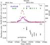 |
Fig. 1 a) Brown points show the Swift/BAT (15–50 keV) daily light curve (Krimm et al. 2013) with times of NuSTAR and pointed Swift/XRT observations marked (arrows). Purple triangles show the MAXI/GSC (Mihara et al. 2011) daily light curve (4–10 keV), rescaled to mCrab fluxes (right-hand y-axis). b) Hardness ratio of Swift/XRT observations, defined as the count rate of the 4–7 keV band divided by the count rate of the 1–4 keV band. |
2.1. Swift
NASA’s Swift satellite (Gehrels et al. 2004, 2005) was launched as a Medium Explorer mission in 2004. Its scientific payload consists of the Burst Alert Telescope (BAT, Barthelmy et al. 2005), the X-ray Telescope (XRT, Burrows et al. 2005), and the Ultraviolet/Optical Telescope (UVOT, Roming et al. 2005). The Swift satellite conducts a continuous all-sky survey in the hard X-rays with the BAT, and is also capable of pointed observations with higher spectral and spatial resolution.
The XRT uses a grazing incidence Wolter type I telescope and a charge coupled device (CCD) sensitive in the energy range of 0.2–10 keV. The XRT operates in different observing modes, resulting in different read-out times, that are appropriate for different flux levels. The effective area of the XRT is more than 120 cm2 at 1.5 keV.
Swift/XRT took ten ~1 ks snapshot observations of A 0535+26 in February and March 2015 (Table 1). All observations were taken in Windowed Timing Mode, which provides a time resolution of 1.7 ms, but only one spatial dimension. We discarded ObsID 00035066058 because the source could not be localized on the chip. We used HEAsoft v. 6.18 and CalDB v. 20160121 for data reprocessing and extraction. Source and background regions are stripes of 96′′ width, centered at the source position and at the outer areas of the chip, respectively. None of the observations was affected by pile-up.
2.2. NuSTAR
The Nuclear Spectroscopic Telescope Array (NuSTAR, Harrison et al. 2013) was launched on 2012 June 13 as a NASA Small Explorer mission. It carries two co-aligned grazing incidence X-ray telescopes and solid-state detectors, sensitive to the energy range of 3–79 keV.
The optics are built of 133 nested shells with a field of view of 10′ × 10′ at 10 keV. The detectors placed in the focal plane of each optical module (called FPM-A and FPM-B) are pixeled CdZnTe detectors which are actively shielded by CsI detectors. The pixels are read out individually upon triggering, which avoids pile-up, a severe problem in many other imaging X-ray detectors employing CCDs. Incident count rates of ~ 105 cts s-1 pixel-1 can in principle be observed without significant pile-up (Harrison et al. 2013), although in practice the maximum event rate that can be detected in a module is limited to ~ 400 s-1, due to to the read-out and processing time of each event. The time resolution is 2 μs (Harrison et al. 2013; Bachetti et al. 2015).
A 0535+26 was observed by NuSTAR on 2015 February 11 and 2015 February 14 (ObsID 80001016002 and 80001016004, hereafter Obs. I and Obs. II, respectively). The data were reprocessed and extracted using the standard NUSTARDAS pipeline v. 1.6 with CalDB version 20161021. Source and background regions are circles with 90′′ radius. All timing information was transferred to the solar barycenter with the FTOOL barycorr and corrected for binary motion according to the ephemeris of Finger et al. (1996) with updated orbital period and epoch2.
Observation log of the NuSTAR and Swift/XRT observations.
3. Timing analysis
We extracted NuSTAR light curves with 413.6 s time resolution for the full 3–78 keV range. In order to avoid variability only due to pulsations, the bin size was chosen to be four times the mean pulse period. The light curves are shown in Fig. 2, together with the hardness ratio, defined here as the count rate of the 15–50 keV band divided by the count rate of the 3–10 keV band. The decrease in count rate over time is clearly visible and Obs. II is softer, in agreement with the long-term trend of the hardness ratio evolution shown in Fig. 1. Both light curves also show moderate variability, which might be due to the well-known strong pulse-to-pulse variability (e.g., Frontera et al. 1985; Klochkov et al. 2011).
We determined the pulse period in both NuSTAR observations using the epoch folding technique (Leahy et al. 1983) applied to 0.5 s resolved light curves. The pulse periods during the NuSTAR observations are 103.3913(8) s in Obs. I and 103.3890(9) s in Obs. II (both at 68% confidence level). Uncertainties on the pulse period were calculated from a set of simulated light curves which are based on the previously determined pulse period and profile with additional Gaussian noise. The pulse period changes only very slightly between the observations and is in excellent agreement with the pulse periods measured around these times by Fermi/GBM (Finger et al. 2009). The Swift observations are too short to constrain the pulse period.
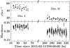 |
Fig. 2 Background-subtracted light curve and hardness ratio for NuSTAR/FPMA data from both observations of A 0535+26. To reduce pulse-phase variations, the time resolution of 413.6 s was chosen to be an integer multiple of the mean pulse period. The hardness ratio is defined as the ratio of the count rate in the 15–50 keV band divided by that of the 3–10 keV band. |
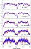 |
Fig. 3 Energy-resolved, background-subtracted pulse profiles of NuSTAR/FPMA for Obs. I (blue) and Obs. II (red). All profiles are normalized such that their mean value is zero and their standard deviation is unity. The pulse profile is repeated for clarity. |
We folded the light curve on the local pulse period to obtain the pulse profiles (Fig. 3). The pulse profiles have been aligned by eye at the pulse minimum. The energy-resolved pulse profiles are very similar in both observations, indicating the same accretion geometry. They show an evolution from a broad plateau-like peak with several very narrow dips at lower energies to a rather smooth, symmetric shape at higher energies.
4. Spectral analysis
Traditionally, continua of accretion-powered X-ray pulsars are described using empirical models which often consist of some power law component with a high-energy cutoff and sometimes an additional soft component. A detailed description of the different empirical models of the exponential turn-over and the terminology used here is given by Müller et al. (2013b).
More sophisticated, physical continuum models aim to calculate the spectral shape by solving the radiative transfer equation for photons passing through the accretion column. Such photons can be generated by bremsstrahlung or blackbody emission, for example, and are then modified by Compton scattering with the electron plasma of the infalling matter. Recently, several physical model implementations have become available. These models rely on slightly different assumptions on the accretion geometry, velocity profile, and emission processes, and also use different techniques to solve the radiation transfer problem. Examples are the compmag model (Farinelli et al. 2012, see Sect. 4.2 for more details) and the Becker & Wolff model (BWmod; Becker & Wolff 2007).
In our analysis, we first apply a sample of different empirical continuum models and compare their characteristics and discuss their success in describing the low-luminosity observations. Then we test a physical continuum model on the data, suitable for the low-luminosity observations reported here. For all fits we used the 1–7 keV and 3.5–79 keV spectra of Swift/XRT and NuSTAR, respectively. We jointly fitted Swift ObsID 00081432001 with NuSTAR Obs. I and Swift ObsID 00035066052 with NuSTAR Obs. II. We rebinned the spectra of FPMA and FPMB jointly, ensuring a minimum signal-to-noise ratio (S/N) of 15 and adding at least 2 and 4 bins together for 3.5–40 keV and 40–79 keV, respectively, in both observations. Swift/XRT spectra were rebinned to a minimum S/N of 15 and 5 for Obs. I and II, respectively. In all fits, detector constants normalized to NuSTAR/FMPA were introduced to account for flux cross-calibration uncertainties between the instruments. Photoelectric absorption is accounted for with the tbnew model, which is an updated version of tbabs3, with abundances and cross sections set according to Wilms et al. (2000) and Verner et al. (1996), respectively.
4.1. Empirical models
The PLCUT model consists of a single power law with photon index Γ and a high-energy cutoff. The parameters determining the cutoff are the folding energy, Efold, and the cutoff energy, Ecut. From the cutoff energy onwards, an exponential decrease in flux is applied on scales of the folding energy, 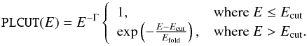 (1)The CutoffPL model is a special case for Ecut = 0. The PLCUT model is not continuously differentiable at the cutoff energy, which can lead to line-like residuals in a spectral fit. Therefore, great caution has to be taken if, for example, additional spectral components such as a CRSF are located close to the cutoff energy. To avoid this issue, the FDCUT cutoff provides a smoother turnover at the cutoff energy. Alternatively, the NPEX model consists of two CutoffPL models with equal folding energy. The second power law has a negative photon index (Makishima et al. 1999; Müller et al. 2013b, and references therein).
4.2. Physical models
In order to describe the spectrum with more physically motivated models, we use the BWmod (Becker & Wolff 2007) and the compmag model of Farinelli et al. (2012).
BWmod is based on a solution of the radiative transfer for a specific velocity profile that is linear in the optical depth (Becker & Wolff 2007). This assumption allows an analytical solution and is well justified for high mass accretion rates where a radiative dominated shock is present. This model was successfully applied to the spectrum of Her X-1 (Wolff et al. 2016) for observations at higher luminosity than that of A 0535+26. As expected, our attempts to fit BWmod to the low-luminosity A 0535+26 data failed. Statistically acceptable fits could be achieved only for the first observation, probably due to the higher number of parameters compared to the empirical models. However, the fits produced parameter combinations that violated underlying assumptions of the model.
The compmag model is better suited to lower luminosity observations. It allows for different velocity profiles, characterized by an index, η, and a terminal velocity, β0, which can be different from zero (Farinelli et al. 2012). The model has been included in XSPEC releases since version 12.8.0. Contrary to BWmod the radiative transfer equation inside the column is solved numerically. While a recent update (Farinelli et al. 2016) adds bremsstrahlung and cyclotron emission as sources for seed photons, we used the 2012 version of the compmag model (Farinelli et al. 2012), where all seed photons are caused by blackbody radiation, with the intention to test a less complex model and because the low-luminosity observations do not necessarily justify the assumption of a radiative dominated shock.
4.3. Cyclotron resonant scattering feature
A 0535+26 is a well-established CRSF source and thus we included an absorption line-like component in our model.
Cyclotron resonant scattering features are typically modeled by Gaussian optical depth line profiles (called gabs in ISIS/XSPEC) or pseudo-Lorentzian profiles (cyclabs; Mihara et al. 1990; Makishima et al. 1990). It should be noted that the width, depth, and line energy are different in the two models (i.e., in the cyclabs model, the line energy ECRSF does not represent where the line is deepest; see Staubert et al. 2014, for a comparison of CRSF energies obtained with different models).
We found that both models provide a satisfactory description of the CRSF feature. We use gabs for the rest of the analysis because of its simplicity and because it has been used in most previous analyses of this source, allowing our results to be directly comparable.
4.4. Results of spectral modeling
We tested the CutoffPL, PLCUT, FDCUT, NPEX, and compmag models. Best-fit parameters are given for empirical models and both observations in Table 2. The spectra with one best-fit model and residuals for all applied models for Obs. I and II are shown in Figs. 4 and 5, respectively. All fit models, except NPEX and compmag, require an additional soft blackbody. Furthermore, a Gaussian emission line with a width fixed to 10-6 keV was included to model the Fe Kα line, thus the line width is only determined by the detector response (~ 400 eV for NuSTAR; Harrison et al. 2013, and ~ 140 eV for Swift/XRT; Burrows et al. 2005). Previous observations have already indicated the presence of a narrow Fe Kα line (Caballero et al. 2007, 2013). We estimated the significance of the inclusion of the iron line with a Monte Carlo approach (see Protassov et al. 2002, for details). Spectra are simulated based on the model without the iron line component and then fitted both with and without the iron line component, and the χ2 difference is compared to the observed one. If the simulated χ2 difference is larger than the observed value we count this as a false-positive detection of the iron line. In both observations, we did not find any false-positive detection in 10 000 simulations, so the significance is >99.99%. For Obs. I the largest simulated χ2 difference is 15.5, while the observed value is 65.4. For Obs. II the largest simulated χ2 difference is 14.4, while the observed value is 16.6.
Best-fit parameters for several empirical models for both observations.
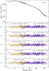 |
Fig. 4 Top panel: unfolded phase-averaged spectrum of Obs. I with best-fit model: XRT (gold), FPMA (blue), FPMB (red), and model for the CutoffPL model (black). All models include an additional narrow iron line. Lower panels: residuals to the different continuum models. For clarity we binned the spectra using larger bins for the plot than the ones used for the fit. |
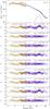 |
Fig. 5 Top panel: unfolded phase-averaged spectrum of Obs. II with the best-fit model: XRT (gold), FPMA (blue), FPMB (red), and model (black). All models include an additional narrow iron line. The gray line shows a decomposition of the CutoffPL and the Gaussian component. Lower panels: residuals to the different continuum models. For clarity we binned the spectra using larger bins for the plot than the ones used for the fit. |
For Obs. I all four empirical continuum models result in statistically acceptable fits. While the PLCUT model produces the lowest χ2 value, its cutoff energy at ~3 keV is so low that this model effectively turns into a CutoffPL model. Discrepancies only occur at very soft energies, where absorption plays a dominant role. Therefore, different continuum models result in slightly different NH values (see Table 2).
This behavior is very different for Obs. II (Fig. 5). In particular, the cutoff sets in much more abruptly than in Obs. I. Over a wide range below the cutoff, the spectrum is almost a pure power law, which bends down around 20–30 keV, although the exact shape of the cutoff is difficult to disentangle from the broad CRSF. The CutoffPL model produces strong residuals at ~30 keV. These residuals also appear when using the FDCUT and NPEX models, although they are less dominant there. Only the PLCUT model describes the data satisfactorily. Alternatively, the sharp turnover can also be modeled by a smooth continuum such as the CutoffPL or FDCUT and an additional broad Gaussian emission component, which is also shown in Fig. 5.
We favor the CutoffPL + Gauss model for Obs. II for further analysis because the NPEX + Gauss and FDCUT + Gauss models produce CRSF parameters that indicate the cutoff is partly modeled by the CRSF. These models are particularly prone to this problem since they include both an emission and an absorption component that are very close in energy. The PLCUT model does not suffer from this disadvantage, but behaves in a fundamentally different way from the other continuum models, which makes its result difficult to compare to previous work.
We assessed the significance of the inclusion of the Gaussian component again using the Monte Carlo approach as described for the iron line. This time, we ran 100 000 simulations for the CutoffPL model and did not find any false-positive detection. The largest simulated χ2 difference was 29.0, which is still very small compared to the observed value of ~ 200. The nominal significance of the feature based on our simulation is therefore >99.999%. If we calculate, however, the probability of a false-positive detection from the χ2 distribution for three degrees of freedom, similar to the approach of Bhalerao et al. (2015), we obtain a significance of >5σ.
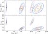 |
Fig. 6 Confidence contours for different fit parameters for Obs. I for the CutoffPL (solid lines) and for the NPEX model (dashed lines). The colors red, green, and blue represent the 68%, 90%, and 99% confidence contours, respectively. |
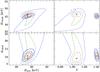 |
Fig. 7 Confidence contours for different fit parameters for Obs. II for the PLCUT (solid lines) and for the CutoffPL + Gauss model (dashed lines). The colors red, green, and blue represent the 68%, 90%, and 99% confidence contours, respectively. |
We find that the CRSF energy only depends marginally on the choice of continuum model. To ensure that possible artificial correlations between the CRSF and the continuum parameters do not affect our conclusions about the CRSF, we calculated confidence contours for several pairs of CRSF and continuum parameters for Obs. I and II, and also compared the different continuum models. The confidence contours for Obs. I and II are shown in Figs. 6 and 7, respectively. In Obs. I, higher folding energies correspond to a stronger CRSF at higher energies, hinting that the exponential roll-over can be partly modeled by the CRSF. However, this correlation is very weak. The CRSF energy is very similar for the CutoffPL and NPEX fits. The different line depths are not unexpected since the photon indices and the folding energies are very different for the two models. Observation II shows well-constrained CRSF parameters for the PLCUT model, and the energy and depth of the CRSF are similar for both the PLCUT and the CutoffPL + Gauss model, although the latter shows an artificial correlation between the continuum parameters photon index and folding energy and the CRSF energy and depth. This behavior is caused by the model containing absorption and emission components being very close to each other in energy.
Similar to the empirical continuum models other than PLCUT, the simple compmag model can only provide a successful description of the first, brighter observation. The second observation shows again clear residuals around 20–30 keV (see Fig. 5). The fit is not acceptable in terms of reduced χ2 and the parameters do not settle at physically meaningful values (e.g., we find accretion column radii that are larger than the canonical neutron star radius, see Table 3). To produce the best fit, we set the flag for the velocity profile to be linear in the optical depth. This is the same assumption as made by (Becker & Wolff 2007) to analytically solve the radiative transfer equation. Similar to the behavior of some of the empirical models, an additional Gaussian emission component at ~ 25 keV also improved the fit of the compmag model to Obs. II. The best-fit parameters are also listed in Table 3.
Best-fit parameters for the compmag model.
As an alternative, we tried to model the spectrum of Obs. II by adding a second Gaussian absorption line at a lower energy than the fundamental CRSF. This approach produces statistically acceptable fits with a  of 0.97 for 804 degrees of freedom. However, the line energy of the low-energy absorption line is
  keV with the CutoffPL model, making it highly unlikely that this feature could be the true fundamental CRSF since no harmonics other than at ~ 45 keV and ~ 100 keV have ever been observed. Furthermore, the line width of
  keV is very wide for a low-energy CRSF and indicates a continuum modeling rather than a true absorption feature. We therefore discard the possibility of a fundamental CRSF at ~ 15 keV.
For direct comparison of the spectral shape of the two observations, in Fig. 8 we show the count rate spectra of NuSTAR-FPMA and the photon flux ratio. Observation II is softer below ~20 keV, but then hardens before the ratio flattens toward higher energies. This behavior is difficult to track beyond ~40 keV, because of the low S/N. The change happens around the Ecut energy in the PLCUT model and the energy of the additional Gaussian in the CutoffPL + Gauss model. The observed softening between Obs. I and II seen in Fig. 2 reflects the excess of soft photons below 10 keV.
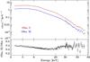 |
Fig. 8 Top: count rate spectra of NuSTAR-FPMA of Obs. I (red) and Obs. II (blue). Bottom: ratio of the count rate spectra. For clarity we binned the spectra using larger bins for the plot than those used for the fit. |
5. Pulse phase-resolved spectroscopy
In order to investigate the variation of the spectral shape with the viewing angle onto the neutron star, we extracted spectra for 12 pulse phase intervals from NuSTAR. The short exposure of the Swift/XRT observations did not allow them to be split further. All pulse phase-resolved spectra of both observations have been rebinned with the same requirements as for the pulse phase-averaged spectra and were restricted to the same energy range.
We fixed the absorption column density to the best-fit value obtained from the phase-averaged spectroscopy with CutoffPL for Obs. I and CutoffPL + Gauss for Obs. II. For all continuum models, the energy of the Fe Kα line is consistent with 6.4 keV and was therefore fixed to that value to reduce the number of free parameters. We kept the line narrow again, fixing its width to 10-6 keV for both observations and all phase bins.
As a result of the lower statistics of the pulse phase-resolved spectra, not all continuum and CRSF parameters can be constrained simultaneously. Generally, we expect variations of all CRSF parameters over pulse phase. The centroid energy of the CRSF may depend on the viewing angle onto the neutron star in a geometrical dipole model (see, e.g., Suchy et al. 2012) or be Doppler shifted, due to viewing angle-dependent components of the bulk motion of the plasma. The pulse phase dependence of the width and depth of the CRSF are, among other effects, a result of the angle dependence of the scattering cross sections (see, e.g., Schwarm et al. 2017b), the plasma temperature, and the emission pattern of the continuum photons. Since preliminary fits showed the CRSF energy to be independent of pulse phase, in our final fits we kept the CSRF energy constant over all phase bins. We caution, however, that fixing of CRSF or continuum parameters might introduce artifacts to the spectral modeling. We also note that Maitra & Paul (2013) observed some variability in the CRSF energy over pulse phase, but had to freeze the CRSF width. We fit all the pulse phase-resolved spectra simultaneously and refer to the parameters that are constant in all phases as “global parameters” (see Kühnel et al. 2015, 2016, for a description of the method).
Although we expect some variation of the CRSF width over pulse phase, as observed in Obs. I, the width of the CRSF could not be constrained in the pulse phase-resolved spectra of Obs. II because of the lower S/N. We therefore fixed the width of the CRSF to the value obtained from the phase-averaged fit since our preliminary fits produced a very wide CRSF. Additionally, we kept the folding energy a global parameter, because it was not well constrained in all phase bins, especially the dim phases.
For Obs. II, the energy and width of the Gaussian emission component only varies marginally with pulse phase, so we kept these parameters global as well. All other parameters were fitted individually for each phase interval. The resulting parameter evolutions are shown in Fig. 9. Reduced χ2 values for the individual phase intervals ranged from 0.95 to 1.22 for Obs. I and 0.94 to 1.38 for Obs. II.
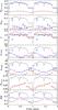 |
Fig. 9 Evolution of some fit parameters over pulse phase for Obs. I (blue) and Obs. II (red). The models used were CutoffPL for Obs. I and CutoffPL + Gauss for Obs. II. The width of the CSRF could not be constrained for individual pulse phases for Obs. II and was therefore kept global. The last panel shows the hardness ratio of the individual phase-resolved spectra, defined as the count rate ratio of the 15–50 keV band divided by the 4–7 keV band. The gray curve shows the 3–78 keV pulse profile of Obs. I to illustrate the selection of the phase intervals. Pulse profile and parameter evolution are shown twice for clarity. All fluxes are given in units of 10-9 erg s-1 cm-2 and the cyclotron line width σCRSF in keV. The light blue data points in phase interval 0.13–0.21 show an alternative fit where the depth of the CRSF was fixed to the mean value of the two neighboring bins, but all global parameters were kept the same. |
The analysis of the phase-resolved spectra is more prone to correlations between model parameters than that of the phase-averaged spectra. This effect is most apparent around phase ~0.17, where the photon index drops and the blackbody flux peaks although the hardness ratio remains rather constant. Fixing the depth of the CRSF for this particular phase interval to the mean value of the neighboring bins, however, the CRSF width and the continuum parameters settle at values favoring the overall evolution of the parameters with pulse phase (Fig. 9, light blue data point).
We obtained the following global parameters: the FPMB normalization constants are 1.004 ± 0.003 and 1.017 ± 0.004, the blackbody temperatures are 1.69 ± 0.03 keV and 1.30 ± 0.02 keV, the folding energies are 32.1 ± 0.3 keV and 22.7 ± 0.2 keV, and the CRSF energies are 47.5 ± 0.3 keV and 43.1 ± 0.5 keV for Obs. I and II, respectively. Additional global parameters for Obs. II are the center and width of the high-energy Gaussian, which are 27.3 ± 0.4 keV and 5.2 ± 0.3 keV, respectively.
6. Discussion
6.1. Timing analysis
The binary corrected pulse period only changes marginally between the two NuSTAR observations. This is to be expected since at this phase of the outburst the mass accretion rate, and therefore the transfer of angular momentum, is very low. Furthermore, the two observations are only ~3 days apart, so intrinsic spin-down should be negligible.
The morphology of the pulse profiles at low energies, as well as their energy dependence, is very similar to those observed during the decay of the 2009 double-peaked outburst when the 3–50 keV luminosity was ~ 1.2 × 1036 erg s-1, which is close to that of the first NuSTAR observation (Caballero et al. 2013).
The pulse profile has been analyzed with a decomposition technique by Caballero et al. (2011). They find that the X-ray pulse profiles are best explained by a hollow accretion column and scattering in a halo around the polar cap.
6.2. Continuum variation and modeling
The pulse phase-averaged spectrum changes significantly between Obs. I and II. While the first, brighter observation can be nicely described with common empirical continuum models and the compmag model, the spectrum of Obs. II shows a very sharp cutoff around 30 keV that cannot be modeled with most standard continuum models. The sharp turnover can be modeled by the PLCUT model, exploiting its abrupt steepening at the cutoff energy Ecut. Alternatively, the “kink” can also be modeled by introducing an additional Gaussian emission component. The Gaussian emission component introduces an additional parameter, but results in slightly better fits than the PLCUT model.
The spectrum of A 0535+26 could be nicely described by power law models with smooth exponential cutoffs over a wide range of luminosities (e.g., Caballero et al. 2007, 2013,for a 3–50 keV luminosity range of 0.04−0.9 × 1037 erg s-1). Sartore et al. (2015) found that the CutoffPL model also describes INTEGRAL observations of A 0535+26 at an estimated bolometric luminosity of ~ 4.9 × 1037 erg s-1. Low-luminosity and quiescence4 observations were taken with RXTE in 1998 and 2011 (Negueruela et al. 2000; Rothschild et al. 2013), with BeppoSAX in 2000 and 2001 (Orlandini et al. 2004). Suzaku observed A 0535+26 in 2005 at a 3–50 keV luminositiy of ~ 3.7 × 1035 erg s-1 (Terada et al. 2006). Terada et al. (2006) successfully used an NPEX continuum model, while Orlandini et al. (2004) and Rothschild et al. (2013) found a pure power law model and a thermal bremsstrahlung model to provide a successful description of the RXTE data. Rothschild et al. caution, however, that the non-detection of an exponential cutoff could be due to the low S/N. Suzaku also observed A 0535+26 in 2009 at a 3–50 keV luminosity of ~ 4 × 1035 erg s-1 (Caballero et al. 2013), at a brightness very similar to the dimmer NuSTAR observation. The phase-averaged spectrum of this observation was modeled with a CutoffPL model (Caballero et al. 2013) and a partially covered NPEX model, power law model, and compTT model (Maitra & Paul 2013). All these fits showed moderate residuals near 30 keV that are similar to those of our fits of Obs. II with the CutoffPL models (Caballero et al. 2013; Maitra & Paul 2013, Figs. 3 and 4, respectively). The two NuSTAR observations presented here are slightly brighter than the 2005 Suzaku observation and cover the luminosity of the dimmest RXTE observations, but provide higher sensitivity compared to Suzaku/PIN and RXTE/PCA. It is therefore very likely that this spectral change would have been unobserved, even if it had happened in previous outbursts.
The luminosity estimates quoted above all used a distance of 2 kpc. This value was derived from spectroscopic measurements (e.g., Hutchings et al. 1978; Giangrande et al. 1980; Steele et al. 1998). Giangrande et al. (1980) report an uncertainty of the spectroscopic distance measurement of 0.6 kpc which introduces a systematic uncertainty of the luminosity of a factor of ~4. Further systematic uncertainties are introduced, for example by assuming isotropic emission, and are discussed in detail in Martínez-Núñez et al. (2017), Kühnel et al. (2017), and Falkner et al. (in prep.).
For further comparison, we show the evolution of the continuum parameters Γ and Efold with the 3–50 keV luminosity of the NuSTAR observations and the RXTE observations of Caballero et al. (2013) in Fig. 10. The RXTE photon index increases toward lower luminosities, which is nicely confirmed with NuSTAR. The folding energy observed by RXTE is constant for luminosities of ~ (3–6) × 1036 erg s-1 and then increases with decreasing luminosity. While the NuSTAR observations are in line with this behavior, they indicate a weaker correlation of the folding energy with luminosity. We note, however, that when fitting the CutoffPL model without the Gaussian emission component to Obs. II, the photon index is harder with similar folding energies. Caballero et al. (2013) also report on a Suzaku observation at a luminosity comparable to the fainter NuSTAR observation. These authors again used a CutoffPL model and found a photon index around ~ 0.84. The fit of NuSTAR Obs. II is significantly improved by adding the Gaussian component (the χ2 changes from 974.9 to 773.3 for the CutoffPL model) and the photon index reflects the softening, also shown in Fig. 2.
This overall softening is in line with earlier work on the spectral behavior of A 0535+26 at lower luminosities. Using RXTE and INTEGRAL data collected in 2010 April at 10–100 keV luminosities of ~ (0.1–1.2) × 1037 erg s-1 in 10–100 keV, Müller et al. (2013a) observed a softening of the photon index and an increase in the folding energy toward lower luminosities. This result confirmed earlier work by Klochkov et al. (2011), who report a spectral softening for decreasing luminosity in their pulse-height-resolved spectroscopy at a luminosity level of around 1038 erg s-1. Owing to lower S/N, Klochkov et al. (2011) had to fix the folding energy to constrain the Γ-luminosity correlation.
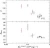 |
Fig. 10 Evolution of the continuum parameters Γ and Efold with the 3–50 keV luminosity. Black data points show the RXTE results of Caballero et al. (2013), and red data points show the result of the NuSTAR observations. The former were obtained using a CutoffPL continuum model, the latter using a CutoffPL and a CutoffPL + Gauss model for Obs. I and II, respectively. |
The physical explanation of this softening at low luminosities is not clear. While spectral formation in accretion columns is an area of active study that started with Basko & Sunyaev (1975) and is under continued refinement (see, e.g., Becker & Wolff 2007; Postnov et al. 2015), few authors focus on spectral formation at very low luminosities. Postnov et al. (2015) observed a softening of the X-ray spectrum toward lower luminosities in a sample of six accreting pulsars and compared this observational result to numerical calculations of the two-dimensional structure of the accretion column with a radiation dominated shock. They focused on luminosities of 1037 erg s-1 and above, and found that the behavior of the spectral hardness is reproduced by Compton saturated emission from an optically thick accretion column. A saturation of the hardness ratio at a few times 1037 erg s-1 was observed and explained by Postnov et al. as a reflection from the neutron star surface; however, their calculations, which are based on the results by Lyubarskii (1986), are only valid for photon energies far below the CRSF energy.
At lower luminosities, Langer & Rappaport (1982) discuss accretion onto highly magnetized (B ~ 1012 G) neutron stars for accretion rates below 1016 g s-1. In this accretion regime, a collision-less shock forms and radiation braking becomes negligible. Langer & Rappaport assume that the spectral distortion of the seed photons due to Comptonization can be neglected. The assumptions for their model are fulfilled by A 0535+26 at the luminosity level of Obs. II (Langer & Rappaport 1982, Eq. (25), where we used the accretion column radii of Table 3). Interestingly, the sample spectrum shown by Langer & Rappaport (1982, their Fig. 4) is based on system properties (B ~ 5 × 10¹² G and Ṁ ~ 5 × 10¹⁵ g s-1) which are very close to those of Obs. II. The predicted spectral shape, however, is clearly different from that observation. The authors argue that most of the energy is emitted in a Doppler-broadened cyclotron emission component, which does not represent the overall power law shape we observe. If the accretion rate decreases even further, the height of the shock is expected to increase and while the emission is still dominated by cyclotron emission, it originates over a wider range along the column. This results in a superposition of different cyclotron energies and forms a smooth continuum with an exponential cutoff above the CRSF energy at the surface. However, comparing their model to the NuSTAR observation reveals significant problems in this interpretation. The observed cutoff energy is below the measured CRSF energy and the spectral shape in the model deviates significantly from a power law below the cutoff energy.
A newer model for the emission of accreting neutron stars at low luminosities has recently been discussed by Vybornov et al. (2017), who studied the behavior of Cep X-4 at luminosities of ~ 1.5 × 1036 erg s-1 and ~ 6 × 1036 erg s-1, i.e., comparable to those the luminosity range studied here for A 0535+26. Vybornov et al. show that the behavior of Cep X-4 at low luminosities can be described using the combination of a collisionless shock and unsaturated Comptonization, rather than undistorted cyclotron emission (Langer & Rappaport 1982). In this Comptonization picture, the spectral shape is like a power law below the CRSF energy, and softens toward low luminosities (Vybornov et al. 2017). Vybornov et al. (2017) show that the evolution of the hardness in Cep X-4, which also shows softening with luminosity, is consistent with this shock picture. Unfortunately, the spectral model used by Vybornov et al. (2017) is not directly applicable to the broadband data used here. By looking at the Compton-y parameter, however, we can test whether the spectral fits found for the compmag model are in the same parameter regime as that claimed for Cep X-4. For a strong magnetic field, the Compton y-parameter is given by (Basko & Sunyaev 1975) 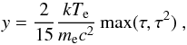 (2)with optical depth, τ, and electron temperature, kTe. Based on the hardness evolution of Cep X-4, Vybornov et al. (2017) find y to range between y = 0.2 and y = 1.2. In contrast, using the compmag parameters from Table 3, we find y ~ (5–8) × 10-4. Taking these values at face value, this result implies Cep X-4 and A 0535+26 to be in different accretion regimes, despite their similar luminosities. We note, however, that the systematic uncertainty of these y values is very large. Given the general behavior seen, however, further work extending the spectral model to the energy range considered here would be very desirable.
Finally, the electron temperatures found in our fits of the spectra of A 0535+26 are comparable to the values given for cases LMC X-4, Cen X-3, and Her X-1 by Becker & Wolff (2007), although these authors considered higher luminosities. It is also close to the application of their model to the spectrum of Her X-1 (Wolff et al. 2016). Farinelli et al. (2016) applied an advanced version of the compmag model to data of Cen X-3, 4U 0115+63, and Her X-1 and found smaller electron temperatures of 0.8–3 keV, which they explained as being due to the inclusion of second order bulk Comptonization in the RTE. Comparing our compmag fits to the successful application of the same version of the model to data of the accreting pulsar RX J0440.9+4431 by Ferrigno et al. (2013), however, the resulting Compton y values are consistently much smaller than unity in both cases (although we find higher optical depths and lower electron temperatures than these authors).
Regarding the Gaussian emission component that is required with the smooth continuum models of the fainter observation, we note that Iwakiri et al. (2012) observed a Gaussian-shaped emission feature during the dim pulse phase of 4U 1626−67. They interpret this feature as the CRSF, which appears in emission only during that particular pulse phase due to the lower optical depth along the line of sight for the corresponding viewing angle. During all other phases and in the phase-averaged spectrum, the CRSF clearly appears in absorption.
This behavior is clearly different from our fainter observation of A 0535+26. The Gaussian emission component is clearly visible in the phase-averaged spectrum, while a CRSF in absorption is still required. In the pulse phase-resolved spectroscopy, the Gaussian emission component is faintest during the dim phases, which is the opposite behavior of what Iwakiri et al. (2012) found.
6.3. Luminosity dependence of the CRSF
One goal of our observations was to investigate the CRSF-luminosity dependence of A 0535+26 toward very low luminosities. As the mass accretion rate changes, we expect changes in the geometry of the accretion column. Since the CRSF energy is representative of the magnetic field strength in the region where most of the radiation is produced, we expect changes in the column geometry to have an impact on the measured line energy (Becker et al. 2012, and references therein). For a long time, no such changes were seen. Observations of many different outbursts over more than two decades have revealed the CRSF line energy to be stable (see, e.g., Kendziorra et al. 1994; Terada et al. 2006; Caballero et al. 2007, 2013). Indications of a positive correlation of the CRSF energy with luminosity were reported by Klochkov et al. (2011) in a pulse-height-resolved analysis of RXTE and INTEGRAL data and by Sartore et al. (2015) using pulse-averaged spectroscopy. The latter authors also observed significant changes in the continuum shape, but had to fix some of the continuum parameters due to strong model-intrinsic parameter correlations. This common approach, however, makes the impact of the continuum variation on the cyclotron line parameters difficult to estimate. All data showing such indications of a positive correlation of the CRSF energy with luminosity were taken at luminosities of ~ 1037 erg s-1 and above.
Previous CRSF observations at low luminosities did not show changes of the CRSF energy with luminosity. It should be noted that the only CRSF observations taken at a luminosity lower than those considered here were taken by Suzaku in 2005 (Terada et al. 2006), and in 2009 (Caballero et al. 2013; Maitra & Paul 2013). Our NuSTAR analysis confirms this result with a much higher precision than was possible with previous missions (see comparison with Terada et al.2006; and Caballero et al.2007, in Fig. 11; and Fig. 4 in Caballero et al.2013).
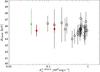 |
Fig. 11 Luminosity dependence of the cyclotron line energy. The black circles and green diamond denote RXTE measurements from Caballero et al. (2007) and Terada et al. (2006), respectively, while the red crosses show the NuSTAR results. The continuum models used to measure the line energy are CutoffPL and PLCUT for Obs. I and Obs. II, respectively. For Obs. II, we used the result of the fit with the PLCUT model. The PLCUT and CutoffPL + Gauss models result in consistent values for ECRSF; however, this value is better constrained in the PLCUT case (Figs. 6 and 7). Terada et al. (2006) and Caballero et al. (2007) used the NPEX and CutoffPL model, respectively. |
The CRSF width is typically around 10 keV (e.g., Caballero 2009; Sartore et al. 2015), which is in good agreement with our results, although smaller line widths have also been reported (e.g., Terada et al. 2006). In contrast, the line depth has been observed to vary significantly between different observations. In principle, such a variability in the depth could be caused by changes in the accretion rate (although the optical depth in the CRSF core is always very high), but we note that the depth depends on the choice of the continuum model (e.g., NPEX produces deeper lines, see Table 2), and caution is advised when comparing data using different continua. At least for the luminosity range covered by Sartore et al. (2015) and by our NuSTAR data, when using the same continuum model the optical depths remain independent of the luminosity.
6.4. Pulse phase-resolved spectroscopy
In the following we discuss the variability of A 0535+26 with the pulse phase. The spectrum is strongly variable in both data sets. Although their absolute values are considerably different, the hardness ratio (see last panel of Fig. 9) shows a similar trend in the two observations.
Of special interest are the phase bins around 0.0 and 0.45, where a large jump in the hardness ratio is seen. While the photon index shows a similar jump at phase 0.0, it hardly deviates from its average value at phase 0.45. We note, however, that the latter behavior could also be due to parameter correlations similar to those discussed in Sect. 5 for the bin around phase ~0.17.
The additional Gaussian emission component around 26 keV in Obs. II is also required for the phase-resolved spectral analysis. The centroid energy and width of this component could not be constrained for each pulse phase interval individually and were therefore kept global throughout the fit. The flux of the Gaussian component varies only moderately over the pulse phase (see Fig. 9) and is of the same order of magnitude as the blackbody flux.
The overall behavior of the source with pulse phase is in line with that discussed by Maitra & Paul (2013) in their pulse phase-resolved spectroscopy of A 0535+26 at a luminosity of ~ 5 × 1035 erg s-1. These authors applied an NPEX and a compTT continuum in a partial covering absorption geometry. They found an increase in the covering fraction and the local absorption component during the main dip of the pulse profile minimum, and associate this with a narrow accretion stream. Owing to NuSTAR’s higher low-energy threshold, our spectral fits did not require a partial covering model, but similar to Maitra & Paul (2013) we find that the hardness ratio has its maximum at the pulse profile minimum, also implying a lack of soft photons at this specific pulse phase.
Turning to spectral components at higher energies, CRSF parameters are expected to vary significantly over the pulse phase as observed in many sources, e.g., in Cen X-3 (Burderi et al. 2000) or 2S 1553−542 (Tsygankov et al. 2016), so fixing any CRSF parameters can introduce artifacts into the spectral modeling. Therefore, a compromise between maximizing S/N, avoiding parameter degeneracies, and capturing intrinsic spectral variability had to be found. We find that, in contrast to other analyses (e.g., Maisack et al. 1997; Maitra & Paul 2013), holding the line energy constant and letting its depth vary results in more consistent results (the width had to be fixed in Obs. II and was left free in Obs. I). This approach is motivated by the assumption that the pulse phase variability of the line is mainly due to changes in the direction of our line of sight onto the CRSF forming region, while still mainly seeing the same emission region and thus magnetic field. In general, the NuSTAR data show that the general behavior of the CRSF is similar in both observations and the CRSF is deepest around the pulse profile minimum. This result is in disagreement with Maitra & Paul (2013), who found the depth of the CRSF to increase with pulse phase during the main peak and then drop significantly around the pulse profile minimum, accompanied by a sudden change in observed CRSF energy. We consider this behavior to be less likely, as our modeling approach does not introduce sudden changes in CRSF parameters with phase.
Next, we try to connect the observed CRSF parameter evolution to an emission geometry. Theoretical calculations and Monte Carlo simulations of cyclotron resonant scattering of photons in an electron plasma predict (Schwarm et al. 2017b, and references therein) that CRSF get wider and shallower when the angle of the photons to the magnetic field in the rest frame of the plasma becomes smaller and narrower, but deeper when the angle to the magnetic field gets larger. This behavior is a result of the width of the peaks of the resonances of the scattering cross sections, which are highly angle-dependent (Schwarm et al. 2017b). This general result is, however, only strictly true for the higher harmonic lines, since the line depth of the fundamental is significantly affected by photon spawning, i.e., the emission of resonant photons during the successive decay of electrons from higher Landau levels, which fill up the fundamental absorption line.
In a very simplified picture we assume pure fan beam emission of the accretion column where the radiation of one accretion column always dominates the observed radiation. Generally, the fan beam emission pattern is supposed to be generated at high luminosities, but a precise luminosity measurement from observational data is very difficult because of numerous systematic uncertainties (Kühnel et al. 2017). The pulse profile shape in the NuSTAR observations is similar to those observed at higher luminosities (e.g., Caballero et al. 2013) so it is unlikely that the emission geometry has changed much compared to higher luminosities. The fan beam scenario is further supported by Caballero et al. (2011) who studied the accretion geometry and emission pattern of A 0535+26 applying a pulse profile decomposition method, although at luminosities of ~ 1037 erg s-1. However, the evaluation of their model, which includes a hollow accretion column, a scattering halo above the neutron star surface, and a complex beam pattern is beyond the scope of current CRSF simulations, although more sophisticated accretion column geometries are very accessible with the Monte Carlo approach (Schwarm et al. 2017a).
One possible result of the fan beam emission can be that indeed most flux is observed at large viewing angles to the B-field and, therefore, that these viewing angles are connected to the pulse profile maximum. We caution that our proposition of the maximum of the pulse profile being connected to large viewing angles due to fan beam emission geometry is a drastic simplification of the highly complex process of pulse profile formation, which includes relativistic effects such as boosting, gravitational light bending, a non-isotropic emission pattern, as well as geometrical properties of the system (e.g., inclination of the B-field and the observer, height, size, and position of the accretion column).
In our observations, the CRSF width has its minimum during the broad peak of the pulse profile. Assuming that small CRSF widths are associated with large viewing angles, as the simulations of CRSF formation mentioned above indicate, this supports the simplified fan beam scenario. We find that changes in the CRSF width and depth with pulse phase are correlated, i.e., the CRSF becomes narrowest and shallowest and vice versa (see Fig. 9). This disagrees with the predictions of simulations because the phase dependence of the width and depth of the CRSF should be determined by the angle to the magnetic field, with opposite angle dependence for the width and depth of the CRSF.
One possible explanation for the unexpected behavior of the CRSF depth could be that the fundamental line is strongly affected by photon spawning of the harmonic lines (the second harmonic at ~100 keV has been observed by, e.g., Kretschmar et al. 1996; Orlandini et al. 2004; Sartore et al. 2015). Furthermore, the excitation rates of fundamental and harmonic lines, and consequently the impact of photon spawning, depend on the hardness of the underlying continuum, which varies with pulse phase. Additionally, different viewing angles may correspond to different optical depths of the column, which strongly determine the observed line depths. Finally, the observed spectrum is the sum of the spectra from two accretion columns seen under different angles, which would further complicate the picture. All these effects could produce an opposite pulse phase dependence of the fundamental CRSF depth from that in the simulations. A proof of this conjecture could be provided by pulse phase-resolved spectroscopy of both the fundamental and the second harmonic, although the latter is not accessible with NuSTAR.
7. Conclusions and outlook
In this paper we have reported on two NuSTAR observations of A 0535+26 at 3–50 keV luminosities of ~ 1.4 × 1036 erg s-1 and ~ 5 × 1035 erg s-1, respectively. These luminosities are comparable to the faintest observations of A 0535+26 taken so far with other instruments (Terada et al. 2006). The quality of the observations allows for a precise measurement of the CRSF parameters and of the continuum. The CRSF energy is in agreement with previous measurements, confirming that the CRSF energy is independent of luminosity over a wide range of luminosities. Together with the constancy of the pulse profile with energy, they probably indicate that the accretion column is stable at these luminosities considered here.
The continuum shape changes significantly between the two observations. While the first, brighter observation is similar in spectral shape to more luminous observations, the second, fainter one shows a kink-like feature around 25 keV that can be modeled either by a an abrupt exponential cutoff or by an additional emission component on top of a smooth continuum. There have been indications of a spectral transition at a luminosity of 0.5–1.0 × 1036 erg s-1 in earlier observations, for example by remaining residuals around 20–30 keV in the Suzaku observation in 2009 (Maitra & Paul 2013; Caballero et al. 2013), but NuSTAR could now resolve this evolution with unprecedented quality. The spectral softening toward lower luminosities found here confirms previous observations. The evolution of the photon index and folding energy is in line with Caballero et al. (2013). A similar behavior of the spectral hardness was reported by Vybornov et al. (2017) for Cep X-4. These authors could reproduce the spectral hardness evolution with an unsaturated Comptonization in a collisionless shock model, however, leading to very different values of the Compton y-parameter.
For a detailed quantitative interpretation of the pulse-phase dependence of the observed spectra, the geometry of the source has to be determined and self-consistent, physical spectral models need to be developed that take the angle- and height-dependence of the emitted radiation into account. One step toward an understanding of the geometry of A 0535+26 was provided by Caballero et al. (2011) who determined the energy-resolved emission pattern of A 0535+26 with a pulse-profile decomposition method. A self-consistent accretion column model that combines continuum and CRSF formation with relativistic effects such as light bending is currently under development (Falkner et al., in prep.).
Observations of the CRSF energy-luminosity dependence and of the dependence of the continuum shape on the luminosity of accreting pulsars over a wide range of luminosities are essential for the further understanding of the structure and formation of the accretion columns since the physical conditions inside the column are expected to depend strongly on the mass accretion rate, which can vary by several orders of magnitude even for individual sources. From an observational point of view, nearby sources such as A 0535+26 or GX 304−1 are of particular interest because they allow observations at very low luminosities at a sufficient S/N with moderate exposure time. The theory of accretion columns has focused mainly on the high-luminosity cases in recent years. We expect additional high-quality observations of accreting pulsars at very low luminosities to foster the development of general theoretical models of low-luminosity accretion on neutron stars.
The relative uncertainty of the parallax of A 0535+26 in Gaia DR1 is ~0.5. For such large uncertainties, the uncertainty of the distance estimate from parallax measurements has a systematic bias (Lutz & Kelker 1973) that does not allow an uncertainty to be assigned to a single parallax derived distance.
An updated period is available through the Fermi/GBM pulsar page https://gammaray.msfc.nasa.gov/gbm/science/pulsars/lightcurves/a0535.html
Acknowledgments
We thank Sebastian Falkner, Matthias Kühnel, and Ingo Kreykenbohm for many fruitful discussions. We thank the Deutsches Zentrum für Luft- und Raumfahrt for support under contract 50 OR 1410. This work was supported under NASA Contract No. NNG08FD60C, and made use of data from the NuSTAR mission, a project led by the California Institute of Technology, managed by the Jet Propulsion Laboratory, and funded by the National Aeronautics and Space Administration. We thank the NuSTAR Operations, Software, and Calibration teams for support with the execution and analysis of these observations. This research has made use of the NuSTAR Data Analysis Software (NuSTARDAS) jointly developed by the ASI Science Data Center (ASDC, Italy) and the California Institute of Technology (USA).
This work has made use of data from the European Space Agency (ESA) mission Gaia (http://www.cosmos.esa.int/gaia), processed by the Gaia Data Processing and Analysis Consortium (DPAC, http://www.cosmos.esa.int/web/gaia/dpac/consortium). Funding for the DPAC has been provided by national institutions, in particular the institutions participating in the Gaia Multilateral Agreement.
This research has made use of a collection of ISIS functions (ISISscripts) provided by ECAP/Remeis observatory and MIT (http://www.sternwarte.uni-erlangen.de/isis/).
References
- Bachetti, M., Harrison, F. A., Cook, R., et al. 2015, ApJ, 800, 109 [NASA ADS] [CrossRef] [Google Scholar]
- Barthelmy, S. D., Barbier, L. M., Cummings, J. R., et al. 2005, Space Sci. Rev., 120, 143 [NASA ADS] [CrossRef] [Google Scholar]
- Basko, M. M., & Sunyaev, R. A. 1975, A&A, 42, 311 [NASA ADS] [Google Scholar]
- Becker, P. A., & Wolff, M. T. 2007, ApJ, 654, 435 [NASA ADS] [CrossRef] [Google Scholar]
- Becker, P. A., Klochkov, D., Schönherr, G., et al. 2012, A&A, 544, A123 [NASA ADS] [CrossRef] [EDP Sciences] [Google Scholar]
- Bhalerao, V., Romano, P., Tomsick, J., et al. 2015, MNRAS, 447, 2274 [NASA ADS] [CrossRef] [Google Scholar]
- Burderi, L., Di Salvo, T., Robba, N. R., La Barbera, A., & Guainazzi, M. 2000, ApJ, 530, 429 [NASA ADS] [CrossRef] [Google Scholar]
- Burrows, D. N., Hill, J. E., Nousek, J. A., et al. 2005, Space Sci. Rev., 120, 165 [NASA ADS] [CrossRef] [Google Scholar]
- Caballero, I. 2009, Ph.D. Thesis, IAAT University of Tuebingen [Google Scholar]
- Caballero, I., Kretschmar, P., Santangelo, A., et al. 2007, A&A, 465, L21 [NASA ADS] [CrossRef] [EDP Sciences] [Google Scholar]
- Caballero, I., Kraus, U., Santangelo, A., Sasaki, M., & Kretschmar, P. 2011, A&A, 526, A131 [NASA ADS] [CrossRef] [EDP Sciences] [Google Scholar]
- Caballero, I., Pottschmidt, K., Marcu, D. M., et al. 2013, ApJ, 764, L23 [NASA ADS] [CrossRef] [Google Scholar]
- Camero-Arranz, A., Finger, M. H., Wilson-Hodge, C. A., et al. 2012, ApJ, 754, 20 [NASA ADS] [CrossRef] [Google Scholar]
- Canuto, V., & Ventura, J. 1977, Fund. Cosmic Phys., 2, 203 [NASA ADS] [Google Scholar]
- Farinelli, R., Ceccobello, C., Romano, P., & Titarchuk, L. 2012, A&A, 538, A67 [NASA ADS] [CrossRef] [EDP Sciences] [Google Scholar]
- Farinelli, R., Ferrigno, C., Bozzo, E., & Becker, P. A. 2016, A&A, 591, A29 [NASA ADS] [CrossRef] [EDP Sciences] [Google Scholar]
- Ferrigno, C., Farinelli, R., Bozzo, E., et al. 2013, A&A, 553, A103 [NASA ADS] [CrossRef] [EDP Sciences] [Google Scholar]
- Finger, M. H., Wilson, R. B., & Harmon, B. A. 1996, ApJ, 459, 288 [NASA ADS] [CrossRef] [Google Scholar]
- Finger, M. H., Beklen, E., Narayana Bhat, P., et al. 2009, ArXiv e-prints [arXiv:0912.3847] [Google Scholar]
- Frontera, F., dal Fiume, D., Morelli, E., & Spada, G. 1985, ApJ, 298, 585 [NASA ADS] [CrossRef] [Google Scholar]
- Gaia Collaboration (Brown, A. G. A., et al.) 2016, A&A, 595, A2 [NASA ADS] [CrossRef] [EDP Sciences] [Google Scholar]
- Gehrels, N., Chincarini, G., Giommi, P., et al. 2004, ApJ, 611, 1005 [NASA ADS] [CrossRef] [Google Scholar]
- Gehrels, N., Chincarini, G., Giommi, P., et al. 2005, ApJ, 621, 558 [NASA ADS] [CrossRef] [Google Scholar]
- Giangrande, A., Giovannelli, F., Bartolini, C., Guarnieri, A., & Piccioni, A. 1980, A&AS, 40, 289 [NASA ADS] [Google Scholar]
- Grove, J. E., Strickman, M. S., Johnson, W. N., et al. 1995, ApJ, 438, L25 [NASA ADS] [CrossRef] [Google Scholar]
- Harrison, F. A., Craig, W. W., Christensen, F. E., et al. 2013, ApJ, 770, 103 [NASA ADS] [CrossRef] [Google Scholar]
- Hutchings, J. B., Bernard, J. E., Crampton, D., & Cowley, A. P. 1978, ApJ, 223, 530 [NASA ADS] [CrossRef] [Google Scholar]
- Iwakiri, W. B., Terada, Y., Mihara, T., et al. 2012, ApJ, 751, 35 [NASA ADS] [CrossRef] [Google Scholar]
- Kendziorra, E., Kretschmar, P., Pan, H. C., et al. 1994, A&A, 291, L31 [NASA ADS] [Google Scholar]
- Klochkov, D., Staubert, R., Santangelo, A., Rothschild, R. E., & Ferrigno, C. 2011, A&A, 532, A126 [NASA ADS] [CrossRef] [EDP Sciences] [Google Scholar]
- Kretschmar, P., Pan, H. C., Kendziorra, E., et al. 1996, A&AS, 120, 175 [NASA ADS] [Google Scholar]
- Krimm, H. A., Holland, S. T., Corbet, R. H. D., et al. 2013, ApJS, 209, 14 [NASA ADS] [CrossRef] [Google Scholar]
- Kühnel, M., Müller, S., Kreykenbohm, I., et al. 2015, Acta Polytechnica, 55, 123 [NASA ADS] [Google Scholar]
- Kühnel, M., Falkner, S., Grossberger, C., et al. 2016, Acta Polytechnica, 56, 41 [Google Scholar]
- Kühnel, M., Fürst, F., Pottschmidt, K., et al. 2017, A&A, 607, A88 [NASA ADS] [CrossRef] [EDP Sciences] [Google Scholar]
- Langer, S. H., & Rappaport, S. 1982, ApJ, 257, 733 [NASA ADS] [CrossRef] [Google Scholar]
- Leahy, D. A., Darbro, W., Elsner, R. F., et al. 1983, ApJ, 266, 160 [NASA ADS] [CrossRef] [Google Scholar]
- Li, F., Clark, G. W., Jernigan, J. G., & Rappaport, S. 1979, ApJ, 228, 893 [NASA ADS] [CrossRef] [Google Scholar]
- Lutz, T. E., & Kelker, D. H. 1973, PASP, 85, 573 [NASA ADS] [CrossRef] [Google Scholar]
- Lyubarskii, Y. É. 1986, Astrophysics, 25, 577 [NASA ADS] [CrossRef] [Google Scholar]
- Maisack, M., Grove, J. E., Kendziorra, E., et al. 1997, A&A, 325, 212 [NASA ADS] [Google Scholar]
- Maitra, C., & Paul, B. 2013, ApJ, 771, 96 [NASA ADS] [CrossRef] [Google Scholar]
- Makishima, K., Ohashi, T., Kawai, N., et al. 1990, PASJ, 42, 295 [NASA ADS] [Google Scholar]
- Makishima, K., Mihara, T., Nagase, F., & Tanaka, Y. 1999, ApJ, 525, 978 [NASA ADS] [CrossRef] [Google Scholar]
- Martínez-Núñez, S., Kretschmar, P., Bozzo, E., et al. 2017, Space Sci. Rev., 212, 59 [NASA ADS] [CrossRef] [Google Scholar]
- Mihara, T., Makishima, K., Ohashi, T., Sakao, T., & Tashiro, M. 1990, Nature, 346, 250 [NASA ADS] [CrossRef] [Google Scholar]
- Mihara, T., Nakajima, M., Sugizaki, M., et al. 2011, PASJ, 63, S623 [Google Scholar]
- Müller, D., Klochkov, D., Caballero, I., & Santangelo, A. 2013a, A&A, 552, A81 [NASA ADS] [CrossRef] [EDP Sciences] [Google Scholar]
- Müller, S., Ferrigno, C., Kühnel, M., et al. 2013b, A&A, 551, A6 [NASA ADS] [CrossRef] [EDP Sciences] [Google Scholar]
- Negueruela, I., Reig, P., Finger, M. H., & Roche, P. 2000, A&A, 356, 1003 [NASA ADS] [Google Scholar]
- Okazaki, A. T., & Negueruela, I. 2001, A&A, 377, 161 [NASA ADS] [CrossRef] [EDP Sciences] [Google Scholar]
- Orlandini, M., Bartolini, C., Campana, S., et al. 2004, Nucl. Phys. B Proc. Suppl., 132, 476 [NASA ADS] [CrossRef] [Google Scholar]
- Postnov, K. A., Gornostaev, M. I., Klochkov, D., et al. 2015, MNRAS, 452, 1601 [NASA ADS] [CrossRef] [Google Scholar]
- Protassov, R., van Dyk, D. A., Connors, A., Kashyap, V. L., & Siemiginowska, A. 2002, ApJ, 571, 545 [NASA ADS] [CrossRef] [Google Scholar]
- Roming, P. W. A., Kennedy, T. E., Mason, K. O., et al. 2005, Space Sci. Rev., 120, 95 [NASA ADS] [CrossRef] [Google Scholar]
- Rosenberg, F. D., Eyles, C. J., Skinner, G. K., & Willmore, A. P. 1975, Nature, 256, 628 [NASA ADS] [CrossRef] [Google Scholar]
- Rothschild, R., Markowitz, A., Hemphill, P., et al. 2013, ApJ, 770, 19 [NASA ADS] [CrossRef] [Google Scholar]
- Sartore, N., Jourdain, E., & Roques, J. P. 2015, ApJ, 806, 193 [NASA ADS] [CrossRef] [Google Scholar]
- Schönherr, G., Wilms, J., Kretschmar, P., et al. 2007, A&A, 472, 353 [NASA ADS] [CrossRef] [EDP Sciences] [Google Scholar]
- Schwarm, F.-W., Ballhausen, R., Falkner, S., et al. 2017a, A&A, 601, A99 [NASA ADS] [CrossRef] [EDP Sciences] [Google Scholar]
- Schwarm, F.-W., Schönherr, G., Falkner, S., et al. 2017b, A&A, 597, A3 [NASA ADS] [CrossRef] [EDP Sciences] [Google Scholar]
- Sina, R. 1996, Ph.D. Thesis, Univ. Maryland [Google Scholar]
- Staubert, R., Klochkov, D., Wilms, J., et al. 2014, A&A, 572, A119 [NASA ADS] [CrossRef] [EDP Sciences] [Google Scholar]
- Steele, I. A., Negueruela, I., Coe, M. J., & Roche, P. 1998, MNRAS, 297, L5 [NASA ADS] [CrossRef] [Google Scholar]
- Suchy, S., Fürst, F., Pottschmidt, K., et al. 2012, ApJ, 745, 124 [NASA ADS] [CrossRef] [Google Scholar]
- Terada, Y., Mihara, T., Nakajima, M., et al. 2006, ApJ, 648, L139 [NASA ADS] [CrossRef] [Google Scholar]
- Tsygankov, S. S., Lutovinov, A. A., Krivonos, R. A., et al. 2016, MNRAS, 457, 258 [NASA ADS] [CrossRef] [Google Scholar]
- Verner, D. A., Ferland, G. J., Korista, K. T., & Yakovlev, D. G. 1996, ApJ, 465, 487 [NASA ADS] [CrossRef] [Google Scholar]
- Vybornov, V., Klochkov, D., Gornostaev, M., et al. 2017, A&A, 601, A126 [NASA ADS] [CrossRef] [EDP Sciences] [Google Scholar]
- Wilms, J., Allen, A., & McCray, R. 2000, ApJ, 542, 914 [NASA ADS] [CrossRef] [Google Scholar]
- Wilson, R. B., Harmon, B. A., Fishman, G. J., & Finger, M. H. 1994, IAU Circ., 5945 [Google Scholar]
- Wolff, M. T., Becker, P. A., Gottlieb, A. M., et al. 2016, ApJ, 831, 194 [NASA ADS] [CrossRef] [Google Scholar]
- Yan, J., Li, H., & Liu, Q. 2012, ApJ, 744, 37 [NASA ADS] [CrossRef] [Google Scholar]
All Tables
All Figures
|
Fig. 1 a) Brown points show the Swift/BAT (15–50 keV) daily light curve (Krimm et al. 2013) with times of NuSTAR and pointed Swift/XRT observations marked (arrows). Purple triangles show the MAXI/GSC (Mihara et al. 2011) daily light curve (4–10 keV), rescaled to mCrab fluxes (right-hand y-axis). b) Hardness ratio of Swift/XRT observations, defined as the count rate of the 4–7 keV band divided by the count rate of the 1–4 keV band. |
| In the text | |
|
Fig. 2 Background-subtracted light curve and hardness ratio for NuSTAR/FPMA data from both observations of A 0535+26. To reduce pulse-phase variations, the time resolution of 413.6 s was chosen to be an integer multiple of the mean pulse period. The hardness ratio is defined as the ratio of the count rate in the 15–50 keV band divided by that of the 3–10 keV band. |
| In the text | |
|
Fig. 3 Energy-resolved, background-subtracted pulse profiles of NuSTAR/FPMA for Obs. I (blue) and Obs. II (red). All profiles are normalized such that their mean value is zero and their standard deviation is unity. The pulse profile is repeated for clarity. |
| In the text | |
|
Fig. 4 Top panel: unfolded phase-averaged spectrum of Obs. I with best-fit model: XRT (gold), FPMA (blue), FPMB (red), and model for the CutoffPL model (black). All models include an additional narrow iron line. Lower panels: residuals to the different continuum models. For clarity we binned the spectra using larger bins for the plot than the ones used for the fit. |
| In the text | |
|
Fig. 5 Top panel: unfolded phase-averaged spectrum of Obs. II with the best-fit model: XRT (gold), FPMA (blue), FPMB (red), and model (black). All models include an additional narrow iron line. The gray line shows a decomposition of the CutoffPL and the Gaussian component. Lower panels: residuals to the different continuum models. For clarity we binned the spectra using larger bins for the plot than the ones used for the fit. |
| In the text | |
|
Fig. 6 Confidence contours for different fit parameters for Obs. I for the CutoffPL (solid lines) and for the NPEX model (dashed lines). The colors red, green, and blue represent the 68%, 90%, and 99% confidence contours, respectively. |
| In the text | |
|
Fig. 7 Confidence contours for different fit parameters for Obs. II for the PLCUT (solid lines) and for the CutoffPL + Gauss model (dashed lines). The colors red, green, and blue represent the 68%, 90%, and 99% confidence contours, respectively. |
| In the text | |
|
Fig. 8 Top: count rate spectra of NuSTAR-FPMA of Obs. I (red) and Obs. II (blue). Bottom: ratio of the count rate spectra. For clarity we binned the spectra using larger bins for the plot than those used for the fit. |
| In the text | |
|
Fig. 9 Evolution of some fit parameters over pulse phase for Obs. I (blue) and Obs. II (red). The models used were CutoffPL for Obs. I and CutoffPL + Gauss for Obs. II. The width of the CSRF could not be constrained for individual pulse phases for Obs. II and was therefore kept global. The last panel shows the hardness ratio of the individual phase-resolved spectra, defined as the count rate ratio of the 15–50 keV band divided by the 4–7 keV band. The gray curve shows the 3–78 keV pulse profile of Obs. I to illustrate the selection of the phase intervals. Pulse profile and parameter evolution are shown twice for clarity. All fluxes are given in units of 10-9 erg s-1 cm-2 and the cyclotron line width σCRSF in keV. The light blue data points in phase interval 0.13–0.21 show an alternative fit where the depth of the CRSF was fixed to the mean value of the two neighboring bins, but all global parameters were kept the same. |
| In the text | |
|
Fig. 10 Evolution of the continuum parameters Γ and Efold with the 3–50 keV luminosity. Black data points show the RXTE results of Caballero et al. (2013), and red data points show the result of the NuSTAR observations. The former were obtained using a CutoffPL continuum model, the latter using a CutoffPL and a CutoffPL + Gauss model for Obs. I and II, respectively. |
| In the text | |
|
Fig. 11 Luminosity dependence of the cyclotron line energy. The black circles and green diamond denote RXTE measurements from Caballero et al. (2007) and Terada et al. (2006), respectively, while the red crosses show the NuSTAR results. The continuum models used to measure the line energy are CutoffPL and PLCUT for Obs. I and Obs. II, respectively. For Obs. II, we used the result of the fit with the PLCUT model. The PLCUT and CutoffPL + Gauss models result in consistent values for ECRSF; however, this value is better constrained in the PLCUT case (Figs. 6 and 7). Terada et al. (2006) and Caballero et al. (2007) used the NPEX and CutoffPL model, respectively. |
| In the text | |
Current usage metrics show cumulative count of Article Views (full-text article views including HTML views, PDF and ePub downloads, according to the available data) and Abstracts Views on Vision4Press platform.
Data correspond to usage on the plateform after 2015. The current usage metrics is available 48-96 hours after online publication and is updated daily on week days.
Initial download of the metrics may take a while.