| Issue |
A&A
Volume 608, December 2017
|
|
|---|---|---|
| Article Number | A122 | |
| Number of page(s) | 18 | |
| Section | Extragalactic astronomy | |
| DOI | https://doi.org/10.1051/0004-6361/201630309 | |
| Published online | 14 December 2017 | |
What does CIVλ1549 tell us about the physical driver of the Eigenvector quasar sequence? ⋆,⋆⋆
1 Instituto de Astrofisíca de Andalucía, IAA-CSIC, 18008 Granada, Spain
e-mail: This email address is being protected from spambots. You need JavaScript enabled to view it.
2 INAF, Osservatorio Astronomico di Padova, IT 35122 Padova, Italy
3 Dipartimento di Fisica & Astronomia “Galileo Galilei”, Univ. of Padova, 35121 Padova, Italy
4 Instituto de Astronomía, UNAM, Mexico DF 04510, Mexico
5 INAF, Osservatorio Astronomico di Bologna, 40129 Bologna, Italy
6 Dept. of Physics & Astronomy, University of Wisconsin, Stevens Points, WI 54481, USA
Received: 21 December 2016
Accepted: 7 August 2017
Abstract
Broad emission lines in quasars enable us to “resolve” structure and kinematics of the broad-line emitting region (BLR) thought to involve an accretion disk feeding a supermassive black hole. Interpretation of broad line measures within the 4DE1 formalism simplifies the apparent confusion among such data by contrasting and unifying properties of so-called high and low accreting Population A and B sources. Hβ serves as an estimator of black hole mass, Eddington ratio and source rest frame; the latter being a valuable input for Civλ1549 studies which allow us to isolate the blueshifted wind component. Optical and HST-UV spectra yield Hβ and Civλ1549 spectra for low-luminosity sources while VLT-ISAAC and FORS and TNG-LRS provide spectra for high-luminosity sources. New high-S/N data for Civ in high-luminosity quasars are presented here for comparison with the other previously published data. Comparison of Hβ and Civλ1549 profile widths/shifts indicates that much of the emission from the two lines arise in regions with different structure and kinematics. Covering a wide range of luminosity and redshift shows evidence for a correlation between Civλ1549 blueshift and source Eddington ratio, with a weaker trend with source luminosity (similar amplitude outflows are seen over four of the five dex luminosity ranges in our combined samples). At low luminosity (z ≲ 0.7) only Population A sources show evidence for a significant outflow while at high luminosity the outflow signature begins to appear in Population B quasars as well.
Key words: quasars: general / quasars: emission lines / quasars: supermassive black holes
Based on observations made with ESO telescopes at the La Silla Paranal Observatory under programme ID082.B-0572(A) and with the Italian Telescopio Nazionale Galileo (TNG) operated by the Fundación Galileo Galilei (INAF) at the Observatorio del Roque de los Muchachos.
The reduced spectra are only available at the CDS via anonymous ftp to cdsarc.u-strasbg.fr (130.79.128.5) or via http://cdsarc.u-strasbg.fr/viz-bin/qcat?J/A+A/608/A122
Present address: Departamento de Matemática Aplicada and IUMA, Universidad de Zaragoza, 50009 Zaragoza, Spain.
© ESO, 2017
1. Introduction
Just over fifty years after their discovery, we are beginning to see progress in both defining and contextualizing the properties of type-1 active galactic nulcei (AGN)/quasars which can be argued to be the “parent population” of the AGN phenomenon. We now know that type-1 sources show considerable diversity in most observed properties. They all show broad optical/UV emission lines from ionic species covering a wide range of ionization potential. Balmer lines (especially Hβ ) and Civλ1549 Å (hereafter Civ) have been used as representatives of low- and high-ionization lines, respectively. They are almost always accompanied by broad permitted Feii emission extending from the far ultraviolet (FUV) to the near infrared (NIR). The Balmer lines have played a prominent role in characterizing the broad-line region (BLR) in lower-redshift (z< 0.8) quasars, with Hβ providing information for the largest number of sources (Osterbrock & Shuder 1982; Wills et al. 1985; Sulentic 1989; Marziani et al. 2003a; Zamfir et al. 2010; Hu et al. 2012; Shen 2013). Most quasars lie beyond z ~ 0.8 where we lose Hβ as a characteristic low-ionization broad line in the absence of expensive IR spectra. Other higher-ionization broad lines appear in their optical spectra. Can any of these lines be used as useful substitute of Hβ ? The higher ionization Civ line has long been considered the best candidate for a BLR diagnostic beyond z ~ 1.4.
Civ and other high-ionization lines – unlike Hβ and other low-ionization lines – frequently show blue-shifted profiles over a broad range in redshift (z) and luminosity (Gaskell 1982; Espey et al. 1989; Tytler & Fan 1992; Marziani et al. 1996; Richards et al. 2002; Bachev et al. 2004; Baskin & Laor 2005; Sulentic et al. 2007; Netzer et al. 2007; Richards et al. 2011; Coatman et al. 2016). The Civ emission line has always played a major role in the study of quasars at z ≳ 1.4. Over the years, we have come to consider outflows as almost ubiquitous in quasars precisely because of the blueshifts of Civ. Early reports at low z encompassed International Ultraviolet Explorer (IUE) observations of individual Seyfert 1 galaxies (e.g., Wamsteker et al. 1990; Zheng et al. 1995), or of high-z quasars with Civ redshifted into the optical band (e.g., Osmer & Smith 1976). Since the 1990s the mainstream interpretation of the blueshift has involved emission by outflowing gas, possibly in a wind (Collin-Souffrin et al. 1988; Emmering et al. 1992; Murray et al. 1995) but alternate interpretations are still being discussed (Gaskell & Goosmann 2013). A less incomplete view came from the first analysis of Hubble Space Telescope (HST) observations (Wills et al. 1993; Corbin & Boroson 1996; Marziani et al. 1996). For the first time, it was possible to take advantage of moderate resolution in the UV domain, and a reliable rest frame set by optical narrow lines. For intermediate to high-z quasars, a turning point came with the first data releases of the Sloan Digital Sky Survey (SDSS; Richards et al. 2002), where shifts were found to be common, especially in the amplitude range from a few hundred km s-1 to ~ 1000 km s-1. It was realized in the 1990s and later confirmed that the behavior of Civ in powerful radio-loud (RL) sources is different from the behavior in radio-quiet (RQ) sources, both in terms of shift amplitude and dependence on luminosity (Marziani et al. 1996; Richards et al. 2011; Marziani et al. 2016a). The previous works suggest that Hβ and Civ are not surrogates of one another – both lines arising, for example, in the same stratified medium (Marziani et al. 2010) and that RQ and RL sources should be considered separately when dealing with a high-ionization line such as Civ. The next major development came with the availability of IR spectrometers that allow the observations of narrow emission lines redshifted into the NIR and therefore to set Civ shifts measurements on a firm quantitative basis. Shifts larger than ~ 1000 km s-1 were found to be frequent at high luminosity (e.g., Coatman et al. 2016; Marziani et al. 2016a; Vietri 2017b; Bisogni et al. 2017).
Current interpretation of the BLR in quasars sees the broad lines arising in a region that is physically and dynamically composite (Collin-Souffrin et al. 1988; Elvis 2000; Ferland et al. 2009; Marziani et al. 2010; Kollatschny & Zetzl 2013; Grier et al. 2013; Du et al. 2016). It appears that we need both Civ and Hβ to effectively characterize the low- and high-ionization gas in the BLR of quasars. For the past 20+ years our group has focused on spectroscopy of type-1 AGN/quasars, with one of our goals being the comparison of Hβ and Civ properties in the same sources. The work has involved two main steps.
1) LOWZ: using a large low-z sample (~160+ sources) we introduced the 4DE1 contextualization to distinguish and unify type-1 quasar diversity. Measures of the Hβ profile width and Civ profile shift were adopted as two of the principal 4DE1 parameters in that formalism (Sulentic et al. 2000a,b, 2002). Comparison of Hβ measures with all high S/N Civ HST-UV spectra (130 sources by 2007) completed the low-redshift study (Sulentic et al. 2007). The 4DE1 formalism serves as a multidimensional set of HR diagrams for type-1 sources (Sulentic et al. 2000a). Broad-line measures, FWHM HβBC and Feii strength, as parameterized by the intensity ratio involving the Feii blue blend at 4570 Å and broad Hβ (i.e., RFeII = I(Feiiλ4570)/I(Hβ )), coupled with measures of the Civ profile velocity displacement, provide three dimensions of the 4DE1 parameter space that are observationally independent and measure different physical aspects (see Marziani et al. 2010, and references therein). Earlier evidence for a correlation between the strength of a soft X-ray excess and some of the above measures (Wang et al. 1996; Boller et al. 1996) also motivated the inclusion Γsoft as a 4DE1 parameter.
This first phase yielded a systematic view of the main observational properties along the 4DE1 sequence, which included parameters ranging from FIR colors to prevalence of radio-loud (RL) sources, to [Oiii]λλ4959, 5007 blueshifts. Low-z SDSS samples (Zamfir et al. 2010) corroborates a 4DE1 main sequence extending from Population A quasars with FWHM Hβ < 4000 km s-1, strong optical FeII emission, a frequent Civ blueshift and soft X-ray excess and, at the other extreme, Population B sources usually showing broader lines, weaker optical FeII and absence of a Civ blueshift or soft X-ray excess (Sulentic et al. 2011; Fraix-Burnet et al. 2017, summarize several parameters that change among the 4DE1 sequence and are therefore systematically different between Pops. A and B).
We suggested that the distinction between NLSy1 and the rest of type-1 AGN was not meaningful, and that, at low z, a break in properties occurs at a larger FWHM(Hβ ), ≈4000 km s-1 distinguishing the two populations, A and B, as narrower and broader (or high and low Eddington ratio) sources, respectively (Sulentic et al. 2011). Eventually, the break was associated with a critical Eddington ratio value (Marziani et al. 2003b), and possibly with a change in accretion disk structure (Sulentic et al. 2014b, and references therein). Eddington ratio (L/LEdd) was suggested by several authors as being the key parameter governing the 4DE1 sequence (e.g., Boroson & Green 1992; Marziani et al. 2001; Kuraszkiewicz et al. 2000; Dong et al. 2009; Ferland et al. 2009; Sun & Shen 2015). The roles of orientation, black hole mass, spin, and line-emitting-gas chemical composition in shaping the observed spectra remain unconvincingly understood to this date (Sulentic et al. 2012, and references therein), especially for RQ sources. Nonetheless, the 4DE1 has offered a consistent organization of quasars’ observational properties whose physical interpretation is still lacunose.
2) High-luminosity, HE sample: the advent of the ESO VLT-ISAAC NIR spectrograph opened up the possibility for obtaining high-S/N spectra for Hβ in much-higher-luminosity quasars at intermediate-to-high redshift. Our extreme L quasar sample was chosen from the Hamburg ESO Survey (Wisotzki et al. 2000) in the range z = 0.9−3.1 and bolometric luminosity log L = 47.4−48.4. We obtained spectra of the Hβ region in 53 sources (Sulentic et al. 2004, 2006; Marziani et al. 2009). Some properties of the emission lines in the Hβ region at high luminosity log L ≳ 47 [erg s-1] are relevant to the interpretation of the results of the present paper. The Hβ profile still supported the dichotomy between narrower and broader sources, with the broader sources showing a redward asymmetry, even more prominent than at low-L. The precise definition of Pop. A and Pop. B is however somewhat blurred at high L, since the minimum full width at half maximum (FWHM) of Hβ significantly increases with source bolometric luminosity (Marziani et al. 2009, hereafter M09).
In this paper we add very high S/N VLT-FORS and TNG-LRS spectral data for Civ of 28 high-luminosity quasars. Earlier high-S/N Civ spectra existed for other quasar samples, but no matter how good the Civ data, measures of Civ profiles remained of uncertain interpretation without a precise determination of the quasar rest frame that we have obtained in our sample from the Hβ spectral region. Accurate z measurement is not easy to obtain from UV broad lines, and redshift determinations from optical survey data, even at z ≳ 1, suffer systematic biases as large as several hundred km s-1 (Hewett & Wild 2010; Shen et al. 2016).
This paper presents new observations and data analysis along with detailed profile decompositions (reported in Sect. 2.1) that become possible with high-S/N spectra. Results from Civ data complete step 2 of our Hβ – Civ study and also allow us a comparison with previous low-redshift work. Our comparisons with low-z sources is unprecedented because we introduce a sample of extreme-luminosity sources with accurate rest-frame estimates as well as spectra with high enough S/N to enable decomposition of Civ into the blueshifted component and the unshifted component Civ counterpart to broad component Hβ . Such comparisons are simply the best clues yet about the relative behavior of Pop. A and B quasars at low and high z and low and high L. Measurements and empirical models of spectra are reported in Sect. 3; they are discussed in Sect. 4 with a focus on the correlations between Civ shifts and luminosity and Eddington ratio (Sect. 4.3), which constrain the physical driver of the outflow (Sect. 4.4). A follow-up paper presents an analysis of possible virial broadening estimators based on rest-frame UV observations.
2. Samples, observations, and data analysis
2.1. Contextualizing our old and new CIV samples
Figure 1 shows the locations in a redshift – absolute magnitude plane of our extreme-luminosity Hamburg-ESO (HE) sample and the low-z comparison sample of 70 radio-quiet quasars (RQ) used in this study. The HE sample, and quasars in the low-z sample above z = 0.2 involve the bright end of the optical luminosity function at their respective redshifts. Quasars with luminosities similar to those in the HE sample do not exist at low redshift. We also included in Fig. 1 a sample of 22 high-redshift (z ~ 2.3) quasars (GTC sample) with luminosities similar to local quasars. Spectra for these sources were obtained with the 10 m GTC telescope (Sulentic et al. 2014a). We were motivated to see if low-luminosity quasars similar to our low-z sample (luminosity analogs with log L = 46.1 ± 0.4) existed at z ~ 2.3 and whether or not they would show differences from their low-z counterparts indicating a role for redshift evolution. The lack of Hβ spectra for this sample required rest frame estimation from UV lines.
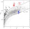 |
Fig. 1 Location of the HE sample in the plane MB vs. redshift (red spots), superimposed to a random subsample of the Véron-Cetty & Véron (2010) catalog (gray dots). Data points representing our low-z RQ control sample and GTC sample of faint quasars at z ~ 2.3 are also shown as black and blue filled circles respectively. The MB associated with two apparent magnitude limited sample (17.5 appropriate for the HE survey, and 21.6 for the SDSS) are shown as a function of redshift. |
2.2. The Hamburg-ESO (HE) sample
Basic sample properties.
2.2.1. General properties
The quasars considered in the present study are selected from ISAAC Hβ observations of 52 quasars identified in the Hamburg ESO survey (Wisotzki et al. 2000), in the redshift range 0.9 ≲ z ≲ 3. Previous observations of Hβ were discussed in a series of papers (Sulentic et al. 2002, 2006; Marziani et al. 2009, hereafter M09). Out of the 52 Hβ sources, 32 have z ≳ 1.4 that allows for coverage of redshifted Civ, and of them, 28 were actually observed.
Table 1 summarizes the main properties of the sources including: identification in the HE catalog, apparent B magnitude taken from Wisotzki et al. (2000), redshift, reference to redshift, absolute K-corrected B magnitude also corrected for Galactic extinction, logarithm of the bolometric luminosity estimated from the tabulated mB, assuming 10λLλ(5100) Å = L, and population assignment (A or B, discussed in Sect. 2.7) in the 4DE1 scheme. In the last column, we identify RL sources. The redshifts were estimated from the narrow component of Hβ and from [Oiii]λλ4959, 5007 (only if consistent with HβNC) and are as reported in M09 and in the previous papers of the series dealing with Hβ VLT/ISAAC observations. They are adopted as systemic redshifts for both the Hβ and Civ spectral range.
2.2.2. Objects belonging to particular classes
HE0512-3329 and HE1104-1805 are known to be gravitationally lensed quasars. They were discussed with the presentation of the Hβ ISAAC spectra (Sulentic et al. 2006). Here we simply note that the FORS1 slit, PA was − 112 deg for HE1104, and that the PA values exclude contamination by the fainter lensed image. The HE0512 PA ≈−41 deg implies an angle with the lens axis of ≈58 deg on average. The small separation between the two lensed images ≈ 0.64 arcsec (which are of comparable brightness in the B-band) implies a separation within the slit of 0.5 arcsec, and that the two images should be well within the slit if the slit was centered on their midpoint. This is however not to be taken for granted since the A component is ≈ 0.44 mag brighter than B in the R band (Gregg et al. 2000). The possibility of lensing or of the occurrence of a close quasar pair was also raised for HE1120+0154 (≡UM 425). In this case, the separation of the FORS observations (≈−171 deg) excludes contamination by fainter lensed quasar images. In addition, the second-brightest component of the lens is very faint, V ≈ 20 (Meylan & Djorgovski 1989).
An interesting aspect of HE1120 is the presence of variable Civ absorption lines (Small et al. 1997). Given the limited radial velocity extent of the absorptions, the source would qualify as a mini-BAL, rather than a BAL QSO since the BALnicity index (Weymann et al. 1991) estimated from our spectrum is 0 km s-1.
HE0359-3959 and HE2352-4010 belong to the class of weak-lined quasars (WLQs, Diamond-Stanic et al. 2009; Shemmer et al. 2010, HE 2352 as a borderline source), for which W(Civ) ≲ 10 Å. WLQs in the HE sample are discussed in Sect. 4.5.
Log of observations.
2.3. Observations and data reduction
Most (24) of the 28 HE quasar observations were obtained with FORS on the 8 m VLT-U2 telescope (ESO, Paranal Observatory, Chile) with four additional observations obtained with the Low Resolution Spectrograph (LRS) at the 3.6 m TNG telescope (Observatorio del Roque de los Muchachos, La Palma, Spain). Table 2 presents an observational log with: equatorial coordinates at J2000, date of observation, telescope and spectrograph, exposure time and slit width in arcsec. Long-slit observations with VLT/FORS1 were obtained with the 600B grism that provided a reciprocal dispersion of 1.5 Å/pixel. The LRS was equipped with the LR-B grism which yielded a dispersion of 2.7 Å/px.
Data reduction was carried out using standard IRAF procedures. Spectra were first trimmed and overscan corrected. Bias subtraction and flat-fielding were performed each night. One dimensional (1D) wavelength calibration using arc lamps were obtained with the same configuration and slit width. The rms of the wavelength calibration was better than 0.07 Å in all cases. The wavelength scales of all individual exposures were realigned with sky lines present in the spectrum before object extraction and background subtraction, to avoid significant zero point errors. The scatter of sky line peak wavelengths after reassignment ≈0.5 Å or 30 km s-1 at 5000 Å provides a realistic estimate of the uncertainty in the wavelength scale. The spectral resolution estimated from the FWHM of skylines is ~200–300 km s-1 for VLT/FORS data. The S/N is ~100–200 in the continuum of the Civ spectral region. The TNG/LRS observations yielded a spectral resolution of ≈600 km s-1 with a typical S/N ≳ 50, and ~200 in the case of HE0926-0201 and HE1409+0101. Flux calibration was obtained each night from spectrophotometric standard stars observed with the same configuration. Due to the narrow slit width, and the wavelength coverage extending to the NUV (≈3300 Å), an additional correction due to differential atmospheric refraction following Filippenko (1982), as well as an absolute flux recalibration, proved to be necessary.
We derived synthetic photometry on the spectra (computed using the sband task of IRAF). Specific fluxes in physical units (erg s-1 cm-2 Å-1) were rescaled to the synoptic Catalina observations (Drake et al. 2009) for the wide majority of the objects, and to the SDSS (HE1120) and the NOMAD catalogs (HE0248; Zacharias et al. 2012; HE0058 and HE0203; Zacharias et al. 2005). Similarly, the original Hβ spectra synthetic magnitudes have been rescaled to the 2MASS J, H, K magnitudes (Cutri et al. 2003). The rescaling allowed for a validation of the bolometric luminosity computed from the 1450 Å and 5100 Å fluxes, assuming bolometric correction factors of 3.5 and 10, respectively. Following the rescaling, the bolometric luminosities derived from the optical and UV are in good agreement, with average δlog L = log (3.5λLλ)1450−log (10λLλ)5100 ≈ −0.072 ± 0.310 (log L ≳ 43.5 [erg s-1]) for the combined LOWZ+HE sample, and δlog L ≈ −0.086 ± 0.264 for the HE sample. Only four sources of the HE sample (HE0205, HE0248, HE0436, and HE0512) have | δlog L | ≳ 0.5. The gravitationally lensed source, HE 0512, might have been affected by a different magnification in the UV and optical. If they are excluded, the HE average becomes δlog L ≈ −0.05 ± 0.17.
Systematic losses in emission line fluxes will cancel out when computing intensity ratios, provided that flux losses are the same for both lines. Nonetheless, great care should be used if computing intensity ratios of individual sources between the Civ and Hβ spectral range. Observations are not simultaneous and separation in time Δt between optical and IR span the range Δτ ≈ Δt/ (1 + z) ≲ 1−3 yr in the rest frame. Major optical/UV variability of highly luminous quasars is expected to occur on long timescales set by the expected emissivity-weighted radius of the BLR,  ld (if we can extrapolate the radius-luminosity relation of Bentz et al. 2009). Previous works have also shown that, for a given time interval, higher-luminosity sources show lower variability levels (Vanden Berk et al. 2004; Simm et al. 2016; Caplar et al. 2017). However, moderate short-term variations (≈20% on Δτ ≈ 15 d on the rest frame) are possible (Woo et al. 2013; Punsly et al. 2016) and, along with intrinsic spectral energy distribution differences affecting the bolometric correction, may be responsible for part of the scatter between rest frame optical- and UV-based L estimates.
2.4. LOWZ: FOS-based comparison sample
A low-L comparison sample was selected from the 71 RQ sources of Sulentic et al. (2007)1. Here we consider 70 RQ FOS sources (one source at log L< 42 erg s-1, with L estimated from the Hβ spectral range, was excluded due to its outlying low luminosity) as a complementary low-L, FOS sample for a comparative analysis of Civ line parameters (LOWZ). Measurements on the Hβ line profiles that include centroids, widths, and asymmetry are available for 49 of them from Marziani et al. (2003a). The comparison is restricted to this sample if Hβ parameters beyond FWHM are involved. RL sources were excluded from the LOWZ sample because they are overrepresented with respect to their prevalence in optically selected samples (≈10%, Zamfir et al. 2008) and especially because radio loudness is affecting the high-ionization outflows traced by Civ (Marziani et al. 1996; Punsly 2010; Richards et al. 2011; Marziani et al. 2016a).
The LOWZ sample cannot be considered complete, but: (1) previous work has shown that it samples well the 4DE1 optical main sequence; and (2) its bolometric luminosity L distribution is relatively uniform over the range 44 ≲ log L ≲ 47 [erg s-1].
2.5. Data analysis: CIVλ1549 and Hβ profile interpretation
The broad profile of the Hβ and Civ profiles in each quasar spectrum can be modeled by changing the relative intensity of three main components.
-
The broad component (BC) has been referred to by variousauthors as the broad component, intermediate component,central broad component (e.g., Brothertonet al. 1994a; Popovićet al. 2002). Here the BC is repre-sented by a symmetric and unshifted profile (Lorentzian forPop. A or Gaussian for Pop. B) andassumed to be associated with a virialized BLR subsystem.
-
The blueshifted component (BLUE). A strong blue excess in Pop. A Civ profiles is not in doubt. In some Civ profiles, such as the extreme Population A prototype I Zw1, the blue excess is by far the dominant contributor to the total emission line flux (Marziani et al. 1996; Leighly & Moore 2004). BLUE is modeled by one or more skew-normal distributions (Azzalini & Regoli 2012). The “asymmetric Gaussian” use is, at present, motivated empirically by the often irregular appearance of the blueshifted excess in Civ and Mgiiλ2800.
-
The very broad component (VBC). We expect a prominent Civ VBC associated with high ionization gas in the innermost BLR (Snedden & Gaskell 2007; Marziani et al. 2010; Wang & Li 2011; Goad & Korista 2014). The VBC was postulated because of typical Hβ profile of Pop. B sources, that can be (empirically) modeled with amazing fidelity using the sum of two Gaussians, one narrower and almost unshifted (the BC) and one broader showing a significant redshift ~ 2000 km s-1 (the VBC, Wills et al. 1993; Brotherton et al. 1994b; Zamfir et al. 2010). Past works provide evidence of a VBC in Civ and other lines (e.g., Marziani et al. 1996; Punsly 2010; Marziani et al. 2010).
In addition, superimposed to the broad profile there is narrower emission most likely associated with larger distances from the central continuum sources (i.e., with the narrow line region, NLR) and unresolved in the FORS spectra. The projected linear size at z ≈ 1.5 is 8.6 kpc/arcsec, meaning that within the ISAAC and FORS, slits were collecting light within a few kpc of the nucleus. This includes not only the innermost part of the NLR but also a significant contribution from the inner bulge of the host galaxy. A fourth component has been considered in the analysis of the integrated Civ and Hβ profiles.
-
The narrow component (NC). The HβNC is not inquestion even in the HE sample, althoughthe ratio HβNC to HβBC is on averagelower at high L. Considering the large projected spatial aper-tures involved in our observations, the spatially-unresolved,emissivity-weighted HβNC is expected to showa relatively narrow profile. The rationale for a significantCivλ1549NC at low-z, and moderate luminositywas provided by Sulentic & Marziani (1999).The lack of a well-defined critical density associated withCiv ([Oiii]λλ4959, 5007 isinstead suppressed at density nH≳106 cm-3) and high ionization, favoringCiv emission, support the assumption thatCiv NC could be up to three times broaderthan [Oiii]λλ4959, 5007 (andHβ ) following the simple model of Net-zer (1990) based on a density radial trend. Hence,the Civλ1549NC profile may merge smoothly withCivBC. Since Civλ1549NC is mainly due to the inner NLRin this scenario, Civλ1549NC blueshifts of a few hun-dred km s-1 persecond are expected. Both Civλ1549NC andHβNC are modeled by a single symmetric Gaussian,but the HβNC is assumed as reference for rest-frame,while Civλ1549NC peak shift is allowed to vary in theCiv profile fits.
2.6. Non-linear multicomponent fits and full-profile measurements of CIVλ1549 and Hβ
The data analysis of the present paper follows the same approach employed in several recent works, and consists in applying a non-linear multicomponent fit to continuum, a scalable Feii emission template, and emission line components (e.g., Negrete et al. 2013; Sulentic et al. 2014a). The minimum  multicomponent fit was carried out with the specfit routine within IRAF (Kriss 1994) yielding FWHM, peak wavelength, and intensity for the four line components BC, BLUE, VBC, and NC. An important caveat is that the line profile models are heuristic because the actual component shapes are unknown.
In addition to the Civ spectra, the Hβ spectral range covered by the VLT-ISAAC was also measured using the IRAF task specfit. The specfit measurements were found to be generally consistent with the earlier ones reported in M092. M09 FWHM,  , and EW of Hβ are on average equal with a scatter ≲20%. Measures toward the line base are influenced by the line profile model; especially on the red side there can be differences associated with the correction by [Oiii]λλ4959, 5007 emission. The correction of M09 was empirical, while in the present paper we assume an intrinsic Hβ broad line shape (Sect. 2.5). This latter approach is preferable because of the strong and irregular [Oiii]λλ4959, 5007 emission recently detected in several luminous quasars (e.g., Cano-Díaz et al. 2012; Carniani et al. 2015; Marziani et al. 2016b, and references therein). The [Oiii]λλ4959, 5007 emission is modeled using a core component plus a semi-broad component, usually blueshifted (e.g., Zhang et al. 2011; Cracco et al. 2016; Marziani et al. 2016b).
Line profile parameters (FWHM, centroids, asymmetry, and kurtosis defined by Zamfir et al. 2010) were measured on the full broad Civ and Hβ profiles (excluding the NC) to provide a qualitative description independent of the specfit modeling. Here we simply stress that line centroids at different fractional peak intensity ( for i = 1,2,3 and c(0.9)) are computed with respect to rest frame, while the asymmetry index (AI) at
  peak line intensity, is computed with respect to the line peak. In addition
  measures the deviations from rest frame close to the line base, while measures the deviations from a symmetric and unshifted line at the fractional intensity where the broadening estimator (the FWHM) is measured. The c(0.9) is used as a proxy for the line peak radial velocity. The mock profiles of Fig. 2 in Marziani et al. (2016a) illustrate the quantitative centroid and width measurements extracted from the broad Civ profile (the narrow component is supposed to have been removed beforehand, if significant). The mock profiles show the main components expected in the Civ profile of Pop. A (BLUE and BC), and Pop. B sources (BLUE, BC, VBC).
2.7. Population classification
The A/B classification of the quasars in HE sample (Table 1) has been assigned by considering a limit in FWHM(Hβ ) following the luminosity-dependent criterion of Sulentic et al. (2004): FWHMAB ≈ 3500 + 500 × 10− 0.06·(MB + 20.24) km s-1, where the MB are reported in Table 1 (see Sulentic et al. 2004, for the derivation of the minimum FWHM as a function of the absolute magnitude).
Given the very weak dependence on L, the luminosity-dependent FWHM separation is consistent with an approximately constant limit at 4000 km s-1 if log L ≲ 47 [erg s-1]. The same population assignments are obtained if the luminosity-dependent limit FWHMAB mentioned in the previous paragraph is applied to FOS sample in place of the constant limit at 4000 km s-1. If virial broadening dominates the width of Hβ , the line emitting region size scales roughly as r ∝ L0.5, and L/LEdd≲ 1, then there is a minimum FWHM corresponding to the maximum L/LEdd. At very high luminosity (log L ≳ 47 [erg s-1]), if all sources radiate sub-Eddington or close to the Eddington limit, we do not expect to observe sources with very narrow lines, such as the one falling in the domain of narrow-line Seyfert 1s (NLSy1s), as further discussed in Sect. 4.2. For instance, at log L ≳ 47 [erg s-1], sources with FWHM ≲ 2500 km s-1 are not possible, if the conditions mentioned earlier in this section are satisfied. At the extreme L ≈ 1015L⊙, no source may show FWHM ≲ 4000 km s-1. This underlines the inadequacy of assuming FWHM = 4000 km s-1 at the typical luminosity of the HE sources. The FWHMAB limit is empirical (as discussed in Sect. 4.5.1 of Marziani et al. 2009). It is found a posteriori that Pop. A and B have systematically different L/LEdd values (Marziani et al. 2003b; Sect. 3.3).
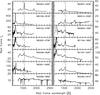 |
Fig. 2 Rest frame UV spectra of the 14 quasars belonging to Pop. A. Abscissae are rest frame wavelength in Å, ordinates are specific flux in units of 10-15 erg s-1 cm-2 Å-1. The dot dashed line traces the rest-frame wavelength of the Civ line. |
With respect to M09 the classification was changed for a few border-line sources close to the luminosity-dependent Pop. A/B boundary: HE1347-2457 and HE2147-3212 → Pop. A (they were previously assigned to spectral type B2, 4000 <FWHM(Hβ ) ≤ 8000 km s-1, 1.0 ≤RFeII≤ 1.5 following Sulentic et al. 2002), HE2156-4020 → Pop. B (was spectral type AM, which includes sources above the canonical limit at FWHM = 4000 km s-1, and below the luminosity-dependent limit for Pop. A as defined in Sulentic et al. 2004).
3. Results
3.1. HE sample CIVλ1549
We identified 14 Pop. A and 14 Pop. B sources in the HE sample. Their rest frame spectra are shown in Figs. 2 and 3, respectively. The first columns of Table 3 report the rest-frame-specific continuum flux fλ at 1450 Å as well as the flux and equivalent width of Civ. The total flux of the 1400 feature (interpreted as a blend of Oiv]λ1402 and Siivλ1397 emission) is reported in the last column; it will not be further considered in the present paper but will be used in a follow-up paper in preparation. Uncertainties on fλ are derived from the magnitude uncertainties used in the rescaling, and are at the 1σ confidence level. Measurements of the integrated line profile for Civ are reported in Table 4 which yields, in the following order: FWHM, asymmetry index, kurtosis, and centroids at and  fractional intensity, along with the uncertainty at 2σ confidence level. The results of the specfit analysis are shown in Figs. 4 and 5 for Pop. A and B sources, respectively. The [Oiii]λλ4959, 5007 emission is modeled with a core and a blueshifted component (Zhang et al. 2011; Marziani et al. 2016b). The Heiiλ1640 emission on the red side of Civ has been modeled with BLUE and BC FWHM and shifts as for Civ, leaving only relative intensities as free parameters. The parameter values for the individual components are listed in Table 5. Flux normalized by the total line flux (including NC), FWHM, and centroid at
  fractional intensity are reported for BLUE, BC, NC, and VBC (the VBC only in the case of Pop. B).
The amplitude of the Civ blueshifts is remarkable. Population A blueshifts exceed 2000 km s-1 in almost all cases, which is a shift amplitude extremely rare at log L ≲ 47 [erg s-1] (Richards et al. 2011). In some extreme cases, the Civ profile appears to be fully blueshifted with respect to the rest frame. Shifts of comparable amplitude are observed only at high luminosity log L ≳ 47 [erg s-1] (e.g., Richards et al. 2011; Coatman et al. 2016, 2017, and references therein). Large shifts above 1000 km s-1 in amplitude are also observed in the Civ profile of most Pop. B sources.
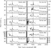 |
Fig. 3 Rest frame UV spectra of the 14 Pop. B HE quasars presented in this paper. Abscissae are rest frame wavelength in Å, ordinates are specific flux in units of 10-15 erg s-1 cm-2 Å-1. |
Spectrophotometric measurements on Civλ1549 and Hβ .
Measurements on the Civλ1549 full line profile.
3.2. HE sample Hβ measurements paired to CIVλ1549
The last four columns of Table 3 report the rest-frame-specific continuum flux fλ at 5100 Å as well as the flux and equivalent width of Hβ and RFeII. As for the UV range, uncertainties on fλ are derived from the magnitude uncertainties used in the rescaling, and are at the 1σ confidence level. The measurements on the Hβ full line profile are reported in Table 6. We note in passing that there is only one source with an apparently discordant Hβ FWHM with respect to its population assignment, HE2349-3800. In this case, the FWHM measurement is not stable, as the profile is the addition of a narrower BC and a much broader VBC (Fig. 5). The asymmetry index AI ≈ 0.3, one of the largest in our sample, places this object among Pop. B sources. Table 7 reports the results of the specfit analysis for Hβ , organized in the same way as for Civ. The new specfit Hβ profile analysis yields results that are consistent with the previous work (M09) on the same objects. VBC shifts are ~ 2000 km s-1 to the red, and the VBC contribution is large, above one half of the total line flux, consistent with the decomposition made by M09 on composite spectra. The large contribution of the VBC makes the BC FWHM especially uncertain.
3.3. HE and LOWZ sample comparison
The meaning of the Civλ1549 properties in the HE sample can be properly evaluated if compared to a low-L sample. The main statistical results from the inter-sample LOWZ-HE comparison are summarized in Table 8 where parameter averages and sample standard deviations are reported for Pops. A and B, along with the statistical significance of the Kolmogorov-Smirnov test, PKS, of the null hypothesis that the HE and LOWZ samples are undistinguishable.
The first two rows list the results for z and UV luminosity λLλ at 1450 Å, which are obviously different at a high significance level. The third parameter listed is the Eddington ratio. The L/LEdd has been computed from the 5100 Å luminosity, assuming a bolometric correction factor of 10 and LEdd ≈ 1.5 × 1038·(MBH/M⊙) erg s-1. The black hole mass MBH was estimated using the same 5100 Å luminosity, the FWHM HβBC with the scaling law of Vestergaard & Peterson (2006). Black hole masses in the HE sample are approximately several 109M⊙, close to the largest MBH values observed in active quasars (Sulentic et al. 2006; Marziani & Sulentic 2012, and references therein) and spent ones in the local Universe (such as Messier 87, Walsh et al. 2013). A L/LEdd systematic difference between LOWZ and HE is present for both Pops. A and B. Indeed, several of the HE Pop. B sources are close to the boundary between Pops. A and B, set from the analysis of low-z quasars. This is, at least in part, the effect of a redshift-dependent L/LEdd bias in a flux limited survey (Sulentic et al. 2014a). In addition, a systematic increase of L/LEdd with z is also expected (Trakhtenbrot & Netzer 2012). The sample difference in L/LEdd is important for interpreting any luminosity difference, and makes it advisable to consider, in addition to Pops. A and B separately, also the full A+B sample (Sect. 4.3).
The second group of rows provides Civ line parameters: FWHM, , , AI, kurtosis and rest frame EW. The third groups provide first the 4DE1 parameters RFeII and FWHM Hβ , and then the profile Hβ parameters reported as for Civ.
We note in passing that the Civ equivalent width is significantly lower for both Pop. A and B, reflecting the well-known anticorrelation between equivalent width of HILs and luminosity (the Baldwin effect e.g., Baldwin et al. 1978; Bian et al. 2012). The Civ EW is also strongly affected by L/LEdd (Bachev et al. 2004; Baskin & Laor 2004; Shemmer & Lieber 2015); this issue will be discussed in a follow-up paper.
The 4DE1 parameter RFeII (third row) is also significantly higher than at low z, but only for Pop. B sources, probably reflecting the increase of RFeII as a function of Eddington ratio (Marziani et al. 2001; Sun & Shen 2015). A similar effect is expected to operate for W(Hβ ), which is systematically higher in Pop. B than in Pop. A at low L: Table 8 indicates a significant decrease in the HE sample, ≈76 Å with respect to ≈100 at low L.
A main result concerning the Civ line profile is that the LOWZ and HE Civ centroids and FWHM are significantly different at a confidence level ≳ 4σ for both Pop. A and B (4th to 6th rows in Table 8). While at low-L a strong effect of the blueshifted excess is restricted mainly to extreme Pop. A sources, at high L the effect of the blueshifted excess is significant also for Pop. B sources, as shown by the profile decomposition of Fig. 5. In the case of the most extreme blueshifts, the kurtosis value can be ≳ 0.4 (Table 4), although sample differences between LOWZ and HE Pops. A and B are never significant (Table 8). On average, profile shape (AI and kurt.) parameters are preserved for both Civ and Hβ .
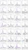 |
Fig. 4 Results of the specfit analysis on the spectra of Pop. A sources in the HE sample, in the Civ and Hβ spectral range (adjacent left and right panels), after continuum subtraction. Horizontal scale is rest frame wavelength in Å or radial velocity shift from Civ rest wavelength (left) or Hβ (right) marked by dot dashed lines; vertical scale is specific flux in units of 10-15 erg s-1 cm-2 Å-1. The panels show the emission line components used in the fit: Feii emission (green), BC (thick black), and BLUE (thick blue), narrow lines (orange). The Oiii]λ1663 line at ≈1660 Å is shown in gray. Thin blue and black lines trace the BLUE and BC for Heiiλ1640. The lower panels show (observed – specfit model) residuals. |
Results of specfit analysis on Civλ1549.
Measurements on the Hβ full line profile.
Results of specfit analysis on Hβ .
Two-sample comparison.
The Civ FWHM is correlated with Civ in Pop. A sources (see Fig. 6; cf. Coatman et al. 2016): 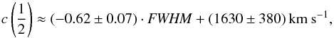 (1)with a significance for the null hypothesis of P ≈ 10-8. The correlation can be straightforwardly explained by the assumption of a blueshifted component of increasing prominence summed to an unshifted symmetric component represented through a scaled Hβ profile, as actually done with the specfit analysis (Sect. 3). The blueshifted excess resolved in radial velocity fully motivates the modelization of the Civ profile as due to the sum of BLUE and BC, and accounts for the Civ FWHM being larger than the FWHM Hβ by almost a factor ≈2 in Pop. A sources (Tables 4 and 6).
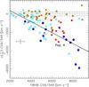 |
Fig. 6 Correlation between Civ FWHM and Civ |
The large Civ blueshifts suggest that in Pop. A sources, the Civ emission is dominated by BLUE: BLUE is  of the Civ total flux for 5 Pop. A objects and ≳ 60% for 9 of them. Conversely, 11 Pop. B sources show I(BLUE) ≲ the total Civ emission I(Civ), and only 3 Pop. B sources have I(BLUE)/I(Civ) ≳ 60% (Table 5). The scheme in Marziani et al. (2016a) indicates that the lower shifts in Pop. B can be ascribed to the combined effect of BLUE plus a BC+VBC profile resembling the one of Hβ .
4. Discussion
4.1. CIV in extreme quasars in 4DE1
The basic picture emerging from the HE sample involves a high prevalence of large Civ shifts, in several cases as large as several thousands km s-1 with respect to the adopted rest frame, and in two cases exceeding 5000 km s-1. Twenty-one out of 24 HE sources show Civ blueshifts larger than 1000 km s-1 (see Table 4). This result is consistent with past finding (e.g., Richards et al. 2011) as well as with more recent works which show that quasars at the highest luminosities (log L ≳ 47 [erg s-1]) display large Civ blueshifts (e.g., Coatman et al. 2016; Vietri 2017b).
A two-population distinction was introduced by several works, on the basis of the Civλ1549 blueshifts (Richards et al. 2011) and of the ratio FWHM to velocity dispersion (Collin et al. 2006; Kollatschny & Zetzl 2011). Population A and B quasars as defined in Sulentic et al. (2000a) provide an effective way to discriminate extremes in quasar properties. Figure 7 shows normalized median composite Civ profiles for the 14 Pop. A (blue) and 14 Pop. B (red) sources where the vertical line represents rest frame wavelength of Civ, derived from the matching Hβ spectra. The median composite profiles presented in Fig. 7 show that Pop. A sources have a stronger signature of a blue component indicative of a wind or outflow. Median composite profiles are a good illustration of the individual blueshift measures presented in Table 4, where the high-luminosity Pop A. profiles show blueshifts with a median of 80% of the flux on the blue side of the rest frame. The fraction of blue component flux among Pop B. sources is 60%, also consistent with the one of the composite. In the comparison LOWZ sample only extreme Pop. A bins (A3, A4) show similar percentage of blueshift flux.
The distributions of the individual values as well as the averages and medians of profile measurements allow a first order comparison of Pop. A–B consistency in the three samples: one of lower L/higher z (GTC) and the other of higher L/higher z (HE), in addition to LOWZ.
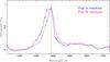 |
Fig. 7 Median composite Civ profiles for the 14 Pop. A (blue line) and 14 Pop. B (red) sources in the HE sample. Vertical line marks the source rest frame derived from the matching Hβ spectra. |
Our LOWZ RQ sample showed Pop. A sources with a median Civ≈− 650 km s-1 while Pop. B showed -230 km s-1 (averages presented in Table 8 yield the same trend). A K-S test indicates a significant difference between the distribution of values of LOWZ Pop. A and B at a 4σ confidence level. The value for low-z Pop. B is close to the typical uncertainty of individual measurements although a ranked-sign test (Dodge 2008) provides a Z-score ≈2.3, for the null hypothesis that the value is not different from 0. In other words, Pop. B sources show modest blueshifts, often within the instrumental uncertainties. Hence our previous inferences that only higher L/LEdd Pop. A quasars show a Civ blueshift (Sulentic et al. 2007). RL sources, which are predominantly Pop. B quasars, are overrepresented in the Hubble archive that provided low-z Civ measures (Wills et al. 1993; Marziani et al. 1996). The median Pop. B Civ shift decreases to − 40 km s-1 if the RL quasars are included. Since the majority of HE (and GTC) quasars are RQ we exclude RLs from comparisons. The GTC sample showed median shifts of − 400 and − 10 km s-1 for Pops. A and B, respectively (significantly different at a ≈ 4σ confidence level), consistent with LOWZ. In the LOWZ and GTC samples, Pop. B spectra show no significant blue flux excess with a large excess for extreme Pop. A sources (Sulentic et al. 2014a). The HE sample shows median Civ shifts of − 2600 and − 1800 km s-1 for Pops. A and B, respectively: Civ is dominated by blueshifted emission although a Pop. A–B difference persists in this high-z, high-L sample (Table 4). The difference between HE and LOWZ is highly significant for both Pops. A and B, as shown by K-S tests whose results are reported in Table 8: the PKS corresponds to a significance level of ≳ 3.5σ, for both Civ and .
Irrespective of whether one interprets the Pop. A and B designations as evidence for two distinct quasar populations (e.g., one capable of radio hyperactivity and one not) or simply a measure of extremes along a 4DE1 sequence, a search for Civ FWHM and profile shift sample differences in the Pop. A–B context gives us more sensitivity to changes due to redshift, luminosity, or Eddington ratio. Figure 8 shows a histogram of Civ shifts in the HE sample. We see that the majority of Pop. A HE sources show large blueshifts and a tendency towards smaller shifts in Pop. B thus preserving profile differences established at low z. However the difference between A and B appears to be decreasing in extreme sources. There may be a selection bias in the HE sample towards sources with higher accretion efficiency but a much larger sample will be needed to prove it (as discussed in Sect. 4.3). In the HE sample, we find only one Pop. B source without a blueshift and a few Pop. A sources with shifts similar to I Zw 1, a A3 prototype extreme blueshift source at low z, with = − 1100 km s-1.
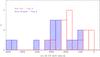 |
Fig. 8 Distribution of Civ profile shifts, |
Full profile FWHM Civ measures for Pop. A and B sources yield medians of 6900 and 6400 km s-1, respectively (averages are ≈6500 km s-1 for both populations, as reported in Table 8). These values are higher than LOWZ medians (with 4130 and 4910 km s-1 for Pop. A and B, respectively) and GTC (≈5200 km s-1 and 5800 km s-1) estimates. The LOWZ and GTC FWHM Civ distributions differ from the HE sample with statistical significance ≳ 4σ. The Civ FWHM in the HE sample is higher for both Pops. A and B due to the growing strength of the wind/outflow component shown in Sect. 3.3 – as Civ blueshift increases, FWHM Civ is likely to increase as well (Fig. 6; see also Fig. 7 in Coatman et al. 2016). This non-virial broadening associated with the wind (e.g., Richards et al. 2011) leads to overestimation of FWHM Civ-based black hole masses (e.g., Netzer et al. 2007; Sulentic et al. 2007; Park et al. 2013; Mejía-Restrepo et al. 2016; Coatman et al. 2017, and references therein). The amplitude of the effect depends on the location of 4DE1 sequence; being stronger for Pop. A (Sulentic et al. 2007; Brotherton et al. 2015).
4.2. The Eigenvector 1 optical plane at low- and high-L
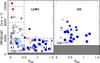 |
Fig. 9 Amplitude of Civ |
Figure 9 incorporates Civ into the 4DE1 optical plane using color to represent the strength of the Civ blueshift. The LOWZ sample (left panel) illustrates the strong preference for Civ blueshifts but only in Pop. A sources and especially sources with higher L/LEdd in bins A2 and A3. Large blueshifts are rare in LOWZ Pop. B. The extreme HE sources presented in this paper (right panel Fig. 9) show a larger fraction of Civ blueshifts due to the blue excess in the Civ profiles of most sources. The FWHM(Hβ ) of HE sample shift upwards as expected if Hβ arises in a structure where profile width is dominated by virial motions (Sect. 2.7; Marziani et al. 2009, a prime candidate is the accretion disk).
The advantage of the present work is to introduce accurate rest frame estimates and S/N high enough to decompose the Civ line profile in a symmetric virialized component and a blue shifted excess at high L. Clear trends then emerge by joining low- and high-L sources which are not even guessed at in low-z samples. The question is now whether the change in the HE sample is driven by L or L/LEdd.
4.3. Is it L or L/LEdd that drives the CIV outflow?
Evidence at low z suggests that Civ is an Eigenvector 1 parameter with L/LEdd likely to be the driver of the wind/outflow. Source luminosity, L, has long been known to be an Eigenvector 2 parameter (Boroson & Green 1992) and therefore not strongly related to any of the 4DE1 parameters which, in low-L samples have been shown to depend more strongly on L/LEdd than on L (Marziani et al. 2003b; Sun & Shen 2015). In other words, luminosity effects are not strong in type-1, and, for a moderate luminosity range (1−2 dex), the diversity of quasars may be mainly accounted for by L/LEdd, along with other parameters not immediately related to L, such as the viewing angle (e.g., Marziani et al. 2001). The addition of Civ measures for extreme HE sources, coupled with our low z sample, makes it possible to search for correlations over the entire range of L/LEdd and over a range of more than 5 dex in quasar luminosity.
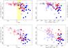 |
Fig. 10 Dependence of Civ |
Results of correlation analysis vs. log L and L/LEdd.
Figure 10 compares the correlations of with L and L/LEdd for 54 Pop A and 45 Pop B quasars in HE and LOWZ samples. We find weak correlation between L and with sources showing large and similar Civ shifts over four of the five dex ranges in source luminosity. Excluding the four extreme blueshifts with log L ≳ 47 [erg s-1], blueshifts between 1000 and 4000 km s-1 are observed over 4 dex in luminosity, as shown in Fig. 10 (upper right). The weak trend is consistent with previous results based on SDSS that found a dependence on luminosity with a large scatter (Richards et al. 2011; Shen et al. 2016). The left panels of Fig. 10 show a clearer trend between L/LEdd and . The largests blueshifts (>1000 km s-1) are observed for L/LEdd≳ 0.2±0.1. In fact the observed distribution of points in the blueshift-L/LEdd diagram supports the suggestion of a discontinuity between L/LEdd and – a critical value of L/LEdd, above which high amplitude winds are possible. If this interpretation is correct, then the Pop. A–B hypothesis would argue that the largest blueshifts are a Pop. A phenomenon and only arise in sources with L/LEdd≳ 0.2. Figure 10 epitomizes a challenging aspect of the Civ blueshift interpretation: on the one hand, largest shifts are observed only at high L, at least in our samples; on the other hand, ≲−1000 km s-1 are not observed at low L/LEdd. This is not to say that outflows do not occur at low L/LEdd, but that the outflowing component BLUE is not dominating the line broadening. The threshold at L/LEdd≈0.2 ± 0.1 would provide a necessary condition for such dominance to occur, with large negative values of possible also at modest L. In other words, high L/LEdd appears the condition sine qua non that makes possible outflows dominating the HIL profiles.
The lower panels of Fig. 10 center the attention on the 72 sources with larger blueshifts (>200 km s-1). The logarithm of || is shown as a function of L/LEdd (left) and L (right) for 42 Pop. A and 30 Pop B sources in the LOWZ and HE samples. The correlation results for the larger blueshift sources are reported in Table 9 where we list the correlation coefficients, computed following Pearson’s definition and the probability of a spurious correlation P. Linear fit parameters (intercept a and slope b), obtained with unweighted least squares (LSQ) and with the orthogonal method (Press et al. 1992) are reported in the following columns. The orthogonal method is known to provide a robust estimator of fit parameters if they are not normally distributed. The values of the Pearson’s correlation coefficient r suggest significant correlations in all cases, at a confidence level > 3σ. The values of r and fitting parameters are listed for Pops. A and B separately first. We then join Pops. A and B to improve the statistics since we do not notice relevant differences between the two populations. A significant correlation (slope b ≈ 0.45 or ≈ 0.58 for LSQ and orthogonal method, respectively) between blueshift Civ and L/LEdd is found. Sources of the joined Pop. A and B sample (last row of Table 9) show an increase in blueshift amplitude with L/LEdd and a Pearson’s correlation coefficient of ≈0.625, corresponding to a confidence level of ≈5.2σ and a probability P ~ 10-7 for the null hypothesis of uncorrelated data. A weaker (slope b ≈ 0.15 for both LSQ and orthogonal method) but still significant dependence of on bolometric L is also found (Fig. 10 bottom right). The luminosity trend becomes appreciable over a very wide range in luminosity (4 dex), when both the LOWZ and HE samples are put together, with Pearson’s correlation coefficient of ≈0.465 implying a confidence level ≈ 3.9σ (Table 9).
The higher frequency of large blueshifts at high luminosity may reflect a bias in L/LEdd distribution of the observable quasars if large shifts are dependent on L/LEdd. The partial correlation coefficient (e.g., Wall & Jenkins 2012) between and L1450 with L/LEdd as a hidden variable is presented in the last column of Table 9, along with its 1σ uncertainty. The partial correlation reveals that, in our sample, the L/LEdd bias is not strong enough to account for the – L correlation: the A+B partial correlation coefficient of – L is significant (at slightly more than 2σ confidence level) if the L/LEdd is considered as the third variable affecting (Table 9). The residual luminosity dependence is rather evident from our data, as blueshifts larger than 2000 km s-1 are not found in the LOWZ sample for λLλ(1450 Å) ≲ 1044 erg s-1. It is unlikely that a large fraction of high-amplitude blueshifts would have gone undetected at 1044 erg s-1≲L ≲ 1047 erg s-1.
4.4. Inferences on the outflowing component dynamical conditions
The main results of the present investigation involve (1) the detection of extreme Civ blueshifts, (2) the dependence of on L/LEdd, and (3) the weaker dependence on luminosity that becomes appreciable over a wide range in luminosity (i.e., large blueshifts in Pop. B at high L even if their L/LEdd is ≲0.3). The threshold above which large Civ blueshifts (≳ 1000 km s-1) are observed may be associated with a change in accretion disk structure: at L/LEdd≳ 0.2, a geometrically and optically thick accretion (“slim”) disk may form in an advection-dominated accretion flow (ADAF; e.g., Abramowicz et al. 1988; Abramowicz & Straub 2014, and references therein). In this case, outflows may be confined at the edge of a funnel (Sa¸dowski et al. 2014), and geometry is expected to favor large shift amplitudes. Estimates of the radiative efficiency suggest that “slim” disks may be very frequent at high-luminosity and high-z where highly accreting quasars are preferentially selected (Netzer & Trakhtenbrot 2014; Trakhtenbrot et al. 2017). The slim configuration may develop in the innermost part of the disk, while further out the disk is expected to retain a radiatively-efficient, geometrically thin regime (e.g., Frank et al. 2002, and references therein). The interplay between wind and the BLR in general and the disk structure at high L/LEdd is a complex problem that it is just beginning to be faced (e.g., Wang et al. 2014, and last paragraph of Sect. 4.5) and that goes beyond the scope of the present paper. In the following, we mainly restrict our discussion to basic considerations on the outflow acceleration mechanism.
Wind models suitable for accretion disks around supermassive black holes can be broadly grouped into two major classes: models based on magnetohydrodynamic centrifugal acceleration (Emmering et al. 1992; Everett 2005; Elitzur et al. 2014), and radiation-driven models (Murray et al. 1995; Elvis 2000; Everett 2005; Proga 2007; Risaliti & Elvis 2010). Both acceleration mechanisms predict that the outflow terminal velocity is strongly dependent on Eddington ratio: for magneto-centrifugal acceleration, the terminal velocity scales as  L/LEdd. This case implies the conservation of the angular momentum of the gas originally in the Keplerian accretion disk. Predicted line profiles are fairly symmetric and often show a prominent core.The second class can more easily account for fully blueshifted profiles as observed in Pop. A sources because radiation-driven winds are expected to give rise to a predominantly radial outflow. Results (1) and (2) also indicate a predominant role of radiative forces, and condition (3) is expected in the case of a radiation-driven outflow.
When radiation forces dominate (which may be the case of a radiation driven wind, or of discrete clouds), the outflow terminal velocity can be written as 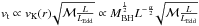 , if r ∝ Lα (e.g., Laor & Brandt 2002; Netzer & Marziani 2010). ℳ is the force multiplier, and vK the Keplerian velocity at the wind launching radius. The slope of the L/LEdd ratio dependence (Table 9) is in agreement with the predictions of a dominant role of radiation forces. A concomitant dependence on luminosity occurs for increasing black hole mass if the term vK or
  depend on luminosity. For example,
  with k ≈ 0.15 is possible if the force multiplier scales roughly with the Eddington ratio.
4.5. Physical conditions of the line emitting gas
The increase in Civ FWHM along with Civ shift argues against a smaller value of the emissivity weighted distance for Civ in a virial velocity field as the dominant broadening effect for Civ; if this were the case, the profile would remain roughly similar to the one of Hβ .
The balance between radiative and gravitational forces is not the same for the whole BLR. Specifically, if we consider the high-ionization and low-ionization lines (HILs and LILs, respectively) emitting BLR as two distinct sub-regions, radiation forces may dominate in the high-ionization sub-region, while gravitational ones in the denser and thicker low-ionization sub-region (Ferland et al. 2009; Marziani et al. 2010; Negrete et al. 2012). The I(CivBC)/I(HβBC) intensity ratio values (which can be deduced from the data reported in Tables 3, 5, and 7) imply low ionization for the gas emitting the virialized BC, and confirm much higher ionization for emission associated with BLUE. The median values for the BC intensity ratios I(Civ)/I(Hβ ) are ≈ 1.4 and ≈ 2.2, and for BLUE I(Civ BLUE)/I(Hβ BLUE) ≈34 and 60 (Pops. A and B, respectively, Tables 5 and 7). The overall scenario envisaged at low z is basically confirmed for the high-z quasars. The low BC I(Civ)/I(Hβ ) along with several other diagnostic flux ratios such as I(Lyα)/I(Civ), I(Aliiiλ1860)/I(Siiii]λ1892), I(Mgiiλ2800)/I(Lyα), I(Feii)/I(Hβ ), and I(Lyα)/I(Hβ ) suggested that the BC is being emitted by a dense region of low-ionization (nH~1011−1012 cm-3, ionization parameter ~ 10-2−10-2.5) while BLUE requires lower density and higher ionization (nH≲1010 cm-3, ionization parameter ~ 10-1, Marziani et al. 2010). The I(Caii)/I(HβBC) intensity ratio measured by Martínez-Aldama et al. (2015) for several sources of the HE sample also indicates the existence of a region of low ionization and high density as the emitter of the BC, and sets a robust lower limit on the density of the line emitting gas, ~ 1010.5 cm-3 (as found by Matsuoka et al. 2007). The inferences on the physical conditions of the two emitting regions add further support to the idea that the emitting gas resolved in radial velocity – that is, emitting BC and BLUE – is also spatially segregated (Collin-Souffrin et al. 1988; Elvis 2000).
Figure 11 shows the relation between and the prominence of BLUE with respect to total Civ emission (upper panel), and the I(CivBC)/I(HβBC) intensity ratio (lower panel). The BLUE prominence and are almost perfectly anti-correlated (Pearson’s r ≈ −0.90), with intensity ratio I(Civ BLUE)/I(Civ) ≈(− 0.15 ± 0.014) + 0.21 ± 0.04, which is not surprising given the definition of BLUE. More interestingly, and the intensity ratio of the broad component of Civ and Hβ are also correlated (r ≈ 0.65): I(CivBC)/I(HβBC) ≈(0.615 ± 0.14) + (3.12 ± 0.36). As the shifts grow larger, the BC of Civ diminishes dramatically. The equivalent width W(Civ) is anti-correlated with and the amplitude is correlated with RFeII (Marziani et al. 2016a): the most extreme shifts are associated with the weakest emission lines, and strongest Feii emitters. In other words, the largest blueshifts are associated with a very low ionization degree: is highly correlated with RFeII: r ≈ −0.82, corresponding to a significance above 4σ for 28 objects. In addition, minimum I(CivBC)/I(HβBC) and the BLUE/Civλ1549 are also associated with the strongest Feii emission: BLUE/Civλ1549 is correlated with RFeII with r ≈ 0.63(3.9σ); and I(CivBC)/I(HβBC) is anti-correlated with r ≈ −0.36 (≈ 2σ). This is why it is so difficult to identify a correction to the FWHM of Civ that is directly connected to : the values are large when blue dominates the Civ emission, and the Civ BC is concomitantly very faint, especially in Pop. A. When the Civ shift is small, however, it might be possible to recover a Civ-based virial estimator. This issue will be the subject of an eventual paper.
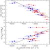 |
Fig. 11 Relation between |
Extreme Pop. A (RFeII≳ 1.0, in the HE sample: HE0122-3759, HE0359-3959, HE1347-2457) all have I(CivBC)/I(HβBC) ≲ 1. The ratio I(CivBC)/I(HβBC) for HE0359-3959 is just ≈ 0.1, since the Civ is almost fully blue shifted. In general, density and ionization parameter appear to reach extreme values in correspondence of sources with RFeII≳ 1, log nH~ 1012 cm-3, and log U ≲ −2.5 (Negrete et al. 2012). These sources (called xA by Marziani & Sulentic 2014) show very low equivalent width of emission lines along the 4DE1 main sequence. Several (but not all; in our sample HE0359-3959 and the borderline object HE2352-4010) meet the definition of weak-lined quasars (WLQs, Diamond-Stanic et al. 2009, W(Civ) ≤ 10 Å). The WLQs in our sample show high-amplitude blueshifts: –5900 (HE0359) and –2390 (HE2352) and also very low I(CivBC)/I(HβBC) ≲ 0.5. WLQs as a class are also characterized by high-amplitude Civλ1549 blueshifts (Plotkin et al. 2015; Shemmer & Lieber 2015). WLQs properties are, in general, consistent with the properties of xA sources. It is interesting to note that WLQ are present also at low L. By joining the Sulentic et al. (2007) and the Plotkin et al. (2015) data, Marziani et al. (2016a) showed that 9 out of 11 sources are consistent with the xA location in the 4DE1 optical plane FWHM(Hβ ) versus RFeII. In turn, xA sources show low W Civ≲ 30 Å could perhaps provide a more appropriate physical limit for isolating the weakest Civλ1549 emitters: WLQs are extreme cases of xA sources but apparently not fundamentally different from the other xA sources, as they show prominent HIL blueshifts along with strong Feii emission.
The results of the present paper yield some constraints on the structure of the BLUE and BC emitting regions in Pop. A. The LIL-BLR may be exposed to a low-level ionizing continuum, due to scatter or self-absorption by the high-ionization wind (not necessarily the same gas emitting the Civ line, e.g., Leighly et al. 2007). An alternative is that the LIL-BLR may be shadowed from the continuum by the optically and geometrically thick structure as provided by an ADAF. At the same time, the 1900 blend of HE sources (described in the follow-up paper) shows a rather high I(Aliiiλ1860)/I(Siiii]λ1892) ratio, implying high density following Negrete et al. (2012). This result suggests that LIL emission may occur from a remnant emitting regions made of the densest gas, while much-lower-density gas is being ablated away and dispersed into the quasar circumnuclear regions.
5. Conclusions
Comparison of low (Hβ ) and high (Civ) excitation broad emission line profiles in high- and low-redshift quasars offers a method to search for quasar evolution in redshift, luminosity, and source Eddington ratio. However there are three desiderata in order to make such comparisons: 1) an accurate measure of the local rest frame in each source, 2) spectral S/N must be high enough to allow decomposition of both Hβ and Civ, and 3) a context in which one can interpret quasar diversity (i.e., Pop. A and B discrimination); this explains why there have been few studies of this kind (e.g., Espey et al. 1989; Marziani et al. 1996; Sulentic et al. 2007; Coatman et al. 2016). Low redshift comparisons show that the two lines are very different in Pop. A and B quasars. This paper combines samples of low-z (ground based/HST-FOS), high-z/low-L (GTC sample) and high-z/high-L (HE ISAAC/FORS and TNG-LRS sample) quasars which explore the full observed ranges of L and L/LEdd. Civ measures of extreme quasars show blueshift values among the largest ever observed. Previously published Hβ spectra provide accurate rest frame measures, Eddington ratios and Pop. A–B classifier while high S/N Civ measures, through accurate line profile decomposition, add insights into disk structure and especially into outflows or winds arising from the disk. Major results are:
-
1.
Civ outflows become stronger and morefrequent at higher z in sources with2−4 dex higher luminosity than low-z quasars. Theemission component associated with the outflow becomes adominant source of line broadening, and confirms that the fullCiv profile is not a useful virial estimator of blackhole mass for most sources.
-
2.
We find that the 4D Eigenvector 1 sequence persists but is less strong among the extreme HE quasars as far as Civ blueshifts are concerned: many Pop B. sources show a significant Civ blueshift. In the optical plane of the 4DE1 parameter space, data points are displaced upwards toward larger FWHM(Hβ ) values, as expected for the systematic increase of line width with luminosity in virialized systems.
-
3.
We show evidence that the Civ outflows are driven by L/LEdd rather than source luminosity. A clear dependence of Civ blueshifts on Eddington ratio is observed while a weaker trend is observed with source luminosity that becomes appreciable only over a wide luminosity range (4–5 dex). Large shifts (
≲− 1000 km s-1) are apparently possible above a threshold L/LEdd≈0.2 ± 0.1. -
4.
The relations between
and L/LEdd and L are consistent with a radiation-driven outflow, and the largest shifts may support the existence of an optically thick ADAF in at least some of the Pop. A sources.
The FOS measurements used in this paper are available on CDS Vizier at http://vizier.u-strasbg.fr
The measurement technique was different for the Hβ observations in M09 and earlier papers by Sulentic et al. (2004) and Sulentic et al. (2006). In those papers Feii and continuum templates were sequentially subtracted before measuring Hβ parameters, and not obtained through a multicomponent nonlinear fit.
Acknowledgments
A.d.O., J.W.S. and M.L.M.A. acknowledge financial support from the Spanish Ministry for Economy and Competitiveness through grants AYA2013-42227-P and AYA2016-76682-C3-1-P. J.P. acknowledges financial support from the Spanish Ministry for Economy and Competitiveness through grants AYA2013-40609-P and AYA2016-76682-C3-3-P. D.D. and A.N. acknowledge support from grants PAPIIT108716, UNAM, and CONACyT221398.
References
- Abramowicz, M. A., & Straub, O. 2014, Scholarpedia, 9, 2408 [NASA ADS] [CrossRef] [Google Scholar]
- Abramowicz, M. A., Czerny, B., Lasota, J. P., & Szuszkiewicz, E. 1988, ApJ, 332, 646 [NASA ADS] [CrossRef] [Google Scholar]
- Azzalini, A., & Regoli, G. 2012, Ann. Inst. Statist. Math., 64, 857 [CrossRef] [Google Scholar]
- Bachev, R., Marziani, P., Sulentic, J. W., et al. 2004, ApJ, 617, 171 [NASA ADS] [CrossRef] [Google Scholar]
- Baldwin, J. A., Burke, W. L., Gaskell, C. M., & Wampler, E. J. 1978, Nature, 273, 431 [NASA ADS] [CrossRef] [Google Scholar]
- Baskin, A., & Laor, A. 2004, MNRAS, 350, L31 [NASA ADS] [CrossRef] [Google Scholar]
- Baskin, A., & Laor, A. 2005, MNRAS, 356, 1029 [NASA ADS] [CrossRef] [Google Scholar]
- Bentz, M. C., Peterson, B. M., Pogge, R. W., & Vestergaard, M. 2009, ApJ, 694, L166 [NASA ADS] [CrossRef] [Google Scholar]
- Bian, W.-H., Fang, L.-L., Huang, K.-L., & Wang, J.-M. 2012, MNRAS, 427, 2881 [NASA ADS] [CrossRef] [Google Scholar]
- Bisogni, S., di Serego Alighieri, S., Goldoni, P., et al. 2017, A&A, 603, A1 [NASA ADS] [CrossRef] [EDP Sciences] [Google Scholar]
- Boller, T., Brandt, W. N., & Fink, H. 1996, A&A, 305, 53 [NASA ADS] [Google Scholar]
- Boroson, T. A., & Green, R. F. 1992, ApJS, 80, 109 [NASA ADS] [CrossRef] [Google Scholar]
- Brotherton, M. S., Wills, B. J., Francis, P. J., & Steidel, C. C. 1994a, ApJ, 430, 495 [NASA ADS] [CrossRef] [Google Scholar]
- Brotherton, M. S., Wills, B. J., Steidel, C. C., & Sargent, W. L. W. 1994b, ApJ, 423, 131 [NASA ADS] [CrossRef] [Google Scholar]
- Brotherton, M. S., Runnoe, J. C., Shang, Z., & DiPompeo, M. A. 2015, MNRAS, 451, 1290 [NASA ADS] [CrossRef] [Google Scholar]
- Cano-Díaz, M., Maiolino, R., Marconi, A., et al. 2012, A&A, 537, L8 [NASA ADS] [CrossRef] [EDP Sciences] [Google Scholar]
- Caplar, N., Lilly, S. J., & Trakhtenbrot, B. 2017, ApJ, 834, 111 [NASA ADS] [CrossRef] [Google Scholar]
- Carniani, S., Marconi, A., Maiolino, R., et al. 2015, A&A, 580, A102 [NASA ADS] [CrossRef] [EDP Sciences] [Google Scholar]
- Coatman, L., Hewett, P. C., Banerji, M., & Richards, G. T. 2016, MNRAS, 461, 647 [NASA ADS] [CrossRef] [Google Scholar]
- Coatman, L., Hewett, P. C., Banerji, M., et al. 2017, MNRAS, 465, 2120 [NASA ADS] [CrossRef] [Google Scholar]
- Collin, S., Kawaguchi, T., Peterson, B. M., & Vestergaard, M. 2006, A&A, 456, 75 [NASA ADS] [CrossRef] [EDP Sciences] [Google Scholar]
- Collin-Souffrin, S., Dyson, J. E., McDowell, J. C., & Perry, J. J. 1988, MNRAS, 232, 539 [NASA ADS] [CrossRef] [Google Scholar]
- Corbin, M. R., & Boroson, T. A. 1996, ApJS, 107, 69 [NASA ADS] [CrossRef] [Google Scholar]
- Cracco, V., Ciroi, S., Berton, M., et al. 2016, MNRAS, 462, 1256 [NASA ADS] [CrossRef] [Google Scholar]
- Cutri, R. M., Skrutskie, M. F., van Dyk, S., et al. 2003, VizieR Online Data Catalog: II/246 [Google Scholar]
- Diamond-Stanic, A. M., Fan, X., Brandt, W. N., et al. 2009, ApJ, 699, 782 [NASA ADS] [CrossRef] [Google Scholar]
- Dodge, Y. 2008, The Concise Encyclopedia of Statistics (Berlin-Heidelberg: Springer Verlag) [Google Scholar]
- Dong, X.-B., Wang, T.-G., Wang, J.-G., et al. 2009, ApJ, 703, L1 [NASA ADS] [CrossRef] [Google Scholar]
- Drake, A. J., Djorgovski, S. G., Mahabal, A., et al. 2009, ApJ, 696, 870 [NASA ADS] [CrossRef] [MathSciNet] [Google Scholar]
- Du, P., Lu, K.-X., Hu, C., et al. 2016, ApJ, 820, 27 [NASA ADS] [CrossRef] [Google Scholar]
- Elitzur, M., Ho, L. C., & Trump, J. R. 2014, MNRAS, 438, 3340 [NASA ADS] [CrossRef] [Google Scholar]
- Elvis, M. 2000, ApJ, 545, 63 [NASA ADS] [CrossRef] [Google Scholar]
- Emmering, R. T., Blandford, R. D., & Shlosman, I. 1992, ApJ, 385, 460 [NASA ADS] [CrossRef] [Google Scholar]
- Espey, B. R., Carswell, R. F., Bailey, J. A., Smith, M. G., & Ward, M. J. 1989, ApJ, 342, 666 [NASA ADS] [CrossRef] [Google Scholar]
- Everett, J. E. 2005, ApJ, 631, 689 [NASA ADS] [CrossRef] [Google Scholar]
- Feigelson, E. D., & Babu, G. J. 1992, ApJ, 397, 55 [NASA ADS] [CrossRef] [Google Scholar]
- Ferland, G. J., Hu, C., Wang, J., et al. 2009, ApJ, 707, L82 [NASA ADS] [CrossRef] [Google Scholar]
- Filippenko, A. V. 1982, PASP, 94, 715 [NASA ADS] [CrossRef] [Google Scholar]
- Fraix-Burnet, D., Marziani, P., D’Onofrio, M., & Dultzin, D. 2017, Frontiers in Astronomy and Space Sciences, 4, 1 [Google Scholar]
- Frank, J., King, A., & Raine, D. J. 2002, Accretion Power in Astrophysics, 3rd edn. (Cambridge: Cambridge University Press) [Google Scholar]
- Gaskell, C. M. 1982, ApJ, 263, 79 [NASA ADS] [CrossRef] [Google Scholar]
- Gaskell, C. M., & Goosmann, R. W. 2013, ApJ, 769, 30 [NASA ADS] [CrossRef] [Google Scholar]
- Goad, M. R., & Korista, K. T. 2014, MNRAS, 444, 43 [NASA ADS] [CrossRef] [Google Scholar]
- Gregg, M. D., Wisotzki, L., Becker, R. H., et al. 2000, AJ, 119, 2535 [NASA ADS] [CrossRef] [Google Scholar]
- Grier, C. J., Peterson, B. M., Horne, K., et al. 2013, ApJ, 764, 47 [NASA ADS] [CrossRef] [Google Scholar]
- Hewett, P. C., & Wild, V. 2010, MNRAS, 405, 2302 [NASA ADS] [Google Scholar]
- Hu, C., Wang, J.-M., Ho, L. C., et al. 2012, ApJ, 760, 126 [NASA ADS] [CrossRef] [Google Scholar]
- Kollatschny, W., & Zetzl, M. 2011, Nature, 470, 366 [NASA ADS] [CrossRef] [Google Scholar]
- Kollatschny, W., & Zetzl, M. 2013, A&A, 549, A100 [NASA ADS] [CrossRef] [EDP Sciences] [Google Scholar]
- Kriss, G. 1994, Astronomical Data Analysis Software and Systems III, ASP Conf. Ser., 61, 437 [NASA ADS] [Google Scholar]
- Kuraszkiewicz, J., Wilkes, B. J., Czerny, B., & Mathur, S. 2000, ApJ, 542, 692 [NASA ADS] [CrossRef] [Google Scholar]
- Laor, A., & Brandt, W. N. 2002, ApJ, 569, 641 [NASA ADS] [CrossRef] [Google Scholar]
- Leighly, K. M., & Moore, J. R. 2004, ApJ, 611, 107 [NASA ADS] [CrossRef] [Google Scholar]
- Leighly, K. M., Halpern, J. P., Jenkins, E. B., et al. 2007, ApJ, 663, 103 [NASA ADS] [CrossRef] [Google Scholar]
- Martínez-Aldama, M. L., Dultzin, D., Marziani, P., et al. 2015, ApJS, 217, 3 [NASA ADS] [CrossRef] [Google Scholar]
- Marziani, P., & Sulentic, J. W. 2012, New Astron. Rev., 56, 49 [NASA ADS] [CrossRef] [Google Scholar]
- Marziani, P., & Sulentic, J. W. 2014, MNRAS, 442, 1211 [NASA ADS] [CrossRef] [Google Scholar]
- Marziani, P., Sulentic, J. W., Dultzin-Hacyan, D., Calvani, M., & Moles, M. 1996, ApJS, 104, 37 [Google Scholar]
- Marziani, P., Sulentic, J. W., Zwitter, T., Dultzin-Hacyan, D., & Calvani, M. 2001, ApJ, 558, 553 [NASA ADS] [CrossRef] [Google Scholar]
- Marziani, P., Sulentic, J. W., Zamanov, R., et al. 2003a, ApJS, 145, 199 [NASA ADS] [CrossRef] [Google Scholar]
- Marziani, P., Zamanov, R. K., Sulentic, J. W., & Calvani, M. 2003b, MNRAS, 345, 1133 [NASA ADS] [CrossRef] [Google Scholar]
- Marziani, P., Sulentic, J. W., Stirpe, G. M., Zamfir, S., & Calvani, M. 2009, A&A, 495, 83 [NASA ADS] [CrossRef] [EDP Sciences] [Google Scholar]
- Marziani, P., Sulentic, J. W., Negrete, C. A., et al. 2010, MNRAS, 409, 1033 [NASA ADS] [CrossRef] [Google Scholar]
- Marziani, P., Martínez Carballo, M. A., Sulentic, J. W., et al. 2016a, Ap&SS, 361, 29 [NASA ADS] [CrossRef] [Google Scholar]
- Marziani, P., Sulentic, J. W., Stirpe, G. M., et al. 2016b, Ap&SS, 361, 3 [NASA ADS] [CrossRef] [Google Scholar]
- Matsuoka, Y., Oyabu, S., Tsuzuki, Y., & Kawara, K. 2007, ApJ, 663, 781 [NASA ADS] [CrossRef] [Google Scholar]
- Mejía-Restrepo, J. E., Trakhtenbrot, B., Lira, P., Netzer, H., & Capellupo, D. M. 2016, MNRAS, 460 [Google Scholar]
- Meylan, G., & Djorgovski, S. 1989, ApJ, 338, L1 [NASA ADS] [CrossRef] [Google Scholar]
- Murray, N., Chiang, J., Grossman, S. A., & Voit, G. M. 1995, ApJ, 451, 498 [NASA ADS] [CrossRef] [Google Scholar]
- Negrete, A., Dultzin, D., Marziani, P., & Sulentic, J. 2012, ApJ, 757, 62 [NASA ADS] [CrossRef] [Google Scholar]
- Negrete, C. A., Dultzin, D., Marziani, P., & Sulentic, J. W. 2013, ApJ, 771, 31 [NASA ADS] [CrossRef] [Google Scholar]
- Netzer, H. 1990, in Active Galactic Nuclei, eds. R. D. Blandford, H. Netzer, L. Woltjer, T. J.-L. Courvoisier, & M. Mayor, 57 [Google Scholar]
- Netzer, H., & Marziani, P. 2010, ApJ, 724, 318 [NASA ADS] [CrossRef] [Google Scholar]
- Netzer, H., & Trakhtenbrot, B. 2014, MNRAS, 438, 672 [NASA ADS] [CrossRef] [Google Scholar]
- Netzer, H., Lira, P., Trakhtenbrot, B., Shemmer, O., & Cury, I. 2007, ApJ, 671, 1256 [NASA ADS] [CrossRef] [Google Scholar]
- Osmer, P. S., & Smith, M. G. 1976, ApJ, 210, 267 [NASA ADS] [CrossRef] [Google Scholar]
- Osterbrock, D. E., & Shuder, J. M. 1982, ApJS, 49, 149 [NASA ADS] [CrossRef] [Google Scholar]
- Park, D., Woo, J.-H., Denney, K. D., & Shin, J. 2013, ApJ, 770, 87 [NASA ADS] [CrossRef] [Google Scholar]
- Plotkin, R. M., Shemmer, O., Trakhtenbrot, B., et al. 2015, ApJ, 805, 123 [NASA ADS] [CrossRef] [Google Scholar]
- Popović, L. Č., Mediavilla, E. G., Kubičela, A., & Jovanović, P. 2002, A&A, 390, 473 [NASA ADS] [CrossRef] [EDP Sciences] [Google Scholar]
- Press, W. H., Teukolsky, S. A., Vetterling, W. T., & Flannery, B. P. 1992, Numerical Recipes in FORTRAN, The Art of Scientific Computing (Cambridge University Press) [Google Scholar]
- Proga, D. 2007, ApJ, 661, 693 [NASA ADS] [CrossRef] [Google Scholar]
- Punsly, B. 2010, ApJ, 713, 232 [NASA ADS] [CrossRef] [Google Scholar]
- Punsly, B., Marziani, P., Zhang, S., Muzahid, S., & O’Dea, C. P. 2016, ApJ, 830, 104 [NASA ADS] [CrossRef] [Google Scholar]
- Richards, G. T., Vanden Berk, D. E., Reichard, T. A., et al. 2002, AJ, 124, 1 [NASA ADS] [CrossRef] [Google Scholar]
- Richards, G. T., Kruczek, N. E., Gallagher, S. C., et al. 2011, AJ, 141, 167 [NASA ADS] [CrossRef] [Google Scholar]
- Risaliti, G., & Elvis, M. 2010, A&A, 516, A89 [NASA ADS] [CrossRef] [EDP Sciences] [Google Scholar]
- Sądowski, A., Narayan, R., McKinney, J. C., & Tchekhovskoy, A. 2014, MNRAS, 439, 503 [NASA ADS] [CrossRef] [Google Scholar]
- Shemmer, O., & Lieber, S. 2015, ApJ, 805, 124 [NASA ADS] [CrossRef] [Google Scholar]
- Shemmer, O., Trakhtenbrot, B., Anderson, S. F., et al. 2010, ApJ, 722, L152 [NASA ADS] [CrossRef] [Google Scholar]
- Shen, Y. 2013, Bull. Astron. Soc. India, 41, 61 [NASA ADS] [Google Scholar]
- Shen, Y., Brandt, W. N., Richards, G. T., et al. 2016, ApJ, 831, 7 [NASA ADS] [CrossRef] [Google Scholar]
- Simm, T., Salvato, M., Saglia, R., et al. 2016, A&A, 585, A129 [NASA ADS] [CrossRef] [EDP Sciences] [Google Scholar]
- Small, T. A., Sargent, W. L. W., & Steidel, C. C. 1997, AJ, 114, 2254 [NASA ADS] [CrossRef] [Google Scholar]
- Snedden, S. A., & Gaskell, C. M. 2007, ApJ, 669, 126 [NASA ADS] [CrossRef] [Google Scholar]
- Sulentic, J. W. 1989, ApJ, 343, 54 [NASA ADS] [CrossRef] [Google Scholar]
- Sulentic, J. W., & Marziani, P. 1999, ApJ, 518, L9 [NASA ADS] [CrossRef] [Google Scholar]
- Sulentic, J. W., Marziani, P., & Dultzin-Hacyan, D. 2000a, ARA&A, 38, 521 [NASA ADS] [CrossRef] [Google Scholar]
- Sulentic, J. W., Marziani, P., Zwitter, T., Dultzin-Hacyan, D., & Calvani, M. 2000b, ApJ, 545, L15 [NASA ADS] [CrossRef] [Google Scholar]
- Sulentic, J. W., Marziani, P., Zamanov, R., et al. 2002, ApJ, 566, L71 [NASA ADS] [CrossRef] [Google Scholar]
- Sulentic, J. W., Stirpe, G. M., Marziani, P., et al. 2004, A&A, 423, 121 [NASA ADS] [CrossRef] [EDP Sciences] [Google Scholar]
- Sulentic, J. W., Repetto, P., Stirpe, G. M., et al. 2006, A&A, 456, 929 [NASA ADS] [CrossRef] [EDP Sciences] [Google Scholar]
- Sulentic, J. W., Bachev, R., Marziani, P., Negrete, C. A., & Dultzin, D. 2007, ApJ, 666, 757 [NASA ADS] [CrossRef] [Google Scholar]
- Sulentic, J., Marziani, P., & Zamfir, S. 2011, Balt. Astron., 20, 427 [NASA ADS] [Google Scholar]
- Sulentic, J. W., Marziani, P., & M., D. 2012, in Fifty Years of Quasars: From Early Observations and Ideas to Future Research, eds. M. D’Onofrio, P. Marziani, & J. W. Sulentic (Berlin-Heidelberg: Springer Verlag), Astrophys. Space Sci. Lib., 386, 549 [Google Scholar]
- Sulentic, J. W., Marziani, P., del Olmo, A., et al. 2014a, A&A, 570, A96 [NASA ADS] [CrossRef] [EDP Sciences] [Google Scholar]
- Sulentic, J. W., Marziani, P., Dultzin, D., D’Onofrio, M., & del Olmo, A. 2014b, J. Phys. Conf. Ser., 565, 012018 [CrossRef] [Google Scholar]
- Sun, J., & Shen, Y. 2015, ApJ, 804, L15 [NASA ADS] [CrossRef] [Google Scholar]
- Trakhtenbrot, B., & Netzer, H. 2012, MNRAS, 427, 3081 [NASA ADS] [CrossRef] [Google Scholar]
- Trakhtenbrot, B., Volonteri, M., & Natarajan, P. 2017, ApJ, 836, L1 [NASA ADS] [CrossRef] [Google Scholar]
- Tytler, D., & Fan, X.-M. 1992, ApJS, 79, 1 [NASA ADS] [CrossRef] [Google Scholar]
- Vanden Berk, D. E., Wilhite, B. C., Kron, R. G., et al. 2004, ApJ, 601, 692 [NASA ADS] [CrossRef] [Google Scholar]
- Véron-Cetty, M.-P., & Véron, P. 2010, A&A, 518, A10 [NASA ADS] [CrossRef] [EDP Sciences] [Google Scholar]
- Vestergaard, M., & Peterson, B. M. 2006, ApJ, 641, 689 [NASA ADS] [CrossRef] [Google Scholar]
- Vietri, G. 2017b, in AAS Meeting Abstracts, 229, 302.06 [Google Scholar]
- Wall, J. V., & Jenkins, C. R. 2012, Practical Statistics for Astronomers (Cambridge: Cambridge University Press) [Google Scholar]
- Walsh, J. L., Barth, A. J., Ho, L. C., & Sarzi, M. 2013, ApJ, 770, 86 [NASA ADS] [CrossRef] [Google Scholar]
- Wamsteker, W., Rodriguez-Pascual, P., Wills, B. J., et al. 1990, ApJ, 354, 446 [NASA ADS] [CrossRef] [Google Scholar]
- Wang, J., & Li, Y. 2011, ApJ, 742, L12 [NASA ADS] [CrossRef] [Google Scholar]
- Wang, T., Brinkmann, W., & Bergeron, J. 1996, A&A, 309, 81 [NASA ADS] [Google Scholar]
- Wang, J.-M., Qiu, J., Du, P., & Ho, L. C. 2014, ApJ, 797, 65 [NASA ADS] [CrossRef] [Google Scholar]
- Weymann, R. J., Morris, S. L., Foltz, C. B., & Hewett, P. C. 1991, ApJ, 373, 23 [NASA ADS] [CrossRef] [Google Scholar]
- Wills, B. J., Netzer, H., & Wills, D. 1985, ApJ, 288, 94 [NASA ADS] [CrossRef] [Google Scholar]
- Wills, B. J., Brotherton, M. S., Fang, D., Steidel, C. C., & Sargent, W. L. W. 1993, ApJ, 415, 563 [NASA ADS] [CrossRef] [Google Scholar]
- Wisotzki, L., Christlieb, N., Bade, N., et al. 2000, A&A, 358, 77 [NASA ADS] [Google Scholar]
- Woo, S. C., Turnshek, D. A., Badenes, C., & Bickerton, S. 2013, MNRAS, 434, 1411 [NASA ADS] [CrossRef] [Google Scholar]
- Zacharias, N., Monet, D. G., Levine, S. E., et al. 2005, VizieR Online Data Catalog: I/297 [Google Scholar]
- Zacharias, N., Finch, C. T., Girard, T. M., et al. 2012, VizieR Online Data Catalog: I/322 [Google Scholar]
- Zamfir, S., Sulentic, J. W., & Marziani, P. 2008, MNRAS, 387, 856 [NASA ADS] [CrossRef] [Google Scholar]
- Zamfir, S., Sulentic, J. W., Marziani, P., & Dultzin, D. 2010, MNRAS, 403, 1759 [NASA ADS] [CrossRef] [Google Scholar]
- Zhang, K., Dong, X.-B., Wang, T.-G., & Gaskell, C. M. 2011, ApJ, 737, 71 [NASA ADS] [CrossRef] [Google Scholar]
- Zheng, W., Kriss, G. A., Davidsen, A. F., et al. 1995, ApJ, 444, 632 [NASA ADS] [CrossRef] [Google Scholar]
All Tables
All Figures
|
Fig. 1 Location of the HE sample in the plane MB vs. redshift (red spots), superimposed to a random subsample of the Véron-Cetty & Véron (2010) catalog (gray dots). Data points representing our low-z RQ control sample and GTC sample of faint quasars at z ~ 2.3 are also shown as black and blue filled circles respectively. The MB associated with two apparent magnitude limited sample (17.5 appropriate for the HE survey, and 21.6 for the SDSS) are shown as a function of redshift. |
| In the text | |
|
Fig. 2 Rest frame UV spectra of the 14 quasars belonging to Pop. A. Abscissae are rest frame wavelength in Å, ordinates are specific flux in units of 10-15 erg s-1 cm-2 Å-1. The dot dashed line traces the rest-frame wavelength of the Civ line. |
| In the text | |
|
Fig. 3 Rest frame UV spectra of the 14 Pop. B HE quasars presented in this paper. Abscissae are rest frame wavelength in Å, ordinates are specific flux in units of 10-15 erg s-1 cm-2 Å-1. |
| In the text | |
|
Fig. 4 Results of the specfit analysis on the spectra of Pop. A sources in the HE sample, in the Civ and Hβ spectral range (adjacent left and right panels), after continuum subtraction. Horizontal scale is rest frame wavelength in Å or radial velocity shift from Civ rest wavelength (left) or Hβ (right) marked by dot dashed lines; vertical scale is specific flux in units of 10-15 erg s-1 cm-2 Å-1. The panels show the emission line components used in the fit: Feii emission (green), BC (thick black), and BLUE (thick blue), narrow lines (orange). The Oiii]λ1663 line at ≈1660 Å is shown in gray. Thin blue and black lines trace the BLUE and BC for Heiiλ1640. The lower panels show (observed – specfit model) residuals. |
| In the text | |
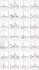 |
Fig. 5 As in Fig. 4, for Pop. B sources, with the addition of the VBC (in red). |
| In the text | |
|
Fig. 6 Correlation between Civ FWHM and Civ |
| In the text | |
|
Fig. 7 Median composite Civ profiles for the 14 Pop. A (blue line) and 14 Pop. B (red) sources in the HE sample. Vertical line marks the source rest frame derived from the matching Hβ spectra. |
| In the text | |
|
Fig. 8 Distribution of Civ profile shifts, |
| In the text | |
|
Fig. 9 Amplitude of Civ |
| In the text | |
|
Fig. 10 Dependence of Civ |
| In the text | |
|
Fig. 11 Relation between |
| In the text | |
Current usage metrics show cumulative count of Article Views (full-text article views including HTML views, PDF and ePub downloads, according to the available data) and Abstracts Views on Vision4Press platform.
Data correspond to usage on the plateform after 2015. The current usage metrics is available 48-96 hours after online publication and is updated daily on week days.
Initial download of the metrics may take a while.