| Issue |
A&A
Volume 606, October 2017
|
|
|---|---|---|
| Article Number | A3 | |
| Number of page(s) | 6 | |
| Section | Cosmology (including clusters of galaxies) | |
| DOI | https://doi.org/10.1051/0004-6361/201731607 | |
| Published online | 22 September 2017 | |
Measuring the cosmic proper distance from fast radio bursts
1 School of Astronomy and Space Science, Nanjing University, 210093 Nanjing, PR China
e-mail: fayinwang@nju.edu.cn (FYW)
2 Key Laboratory of Modern Astronomy and Astrophysics (Nanjing University), Ministry of Education, 210093, Nanjing, PR China
Received: 20 July 2017
Accepted: 23 August 2017
The cosmic proper distance dP is a fundamental distance in the Universe. Unlike the luminosity and angular diameter distances, which correspond to the angular size, the proper distance is the length of light path from the source to observer. However, the proper distance has not been measured before. The recent redshift measurement of a repeat fast radio burst (FRB) can shed light on the proper distance. We show that the proper distance-redshift relation can indeed be derived from dispersion measures (DMs) of FRBs with measured redshifts. From Monte Carlo simulations, we find that about 500 FRBs with DM and redshift measurements can tightly constrain the proper distance-redshift relation. We also show that the curvature of our Universe can be constrained with a model-independent method using this derived proper distance-redshift relation and the observed angular diameter distances. Owing to the high event rate of FRBs, hundreds of FRBs can be discovered in the future by upcoming instruments. The proper distance will play an important role in investigating the accelerating expansion and the geometry of the Universe.
Key words: cosmology: theory / radio continuum: general / cosmological parameters / distance scale / large-scale structure of Universe
© ESO, 2017
1. Introduction
In astronomy, a long-standing and intriguing question is the measurement of distance. There are several distance definitions in cosmology, such as the luminosity distance dL, the angular diameter distance dA, the transverse comoving distance dM, and the proper distance dP (Weinberg 1972; Coles & Lucchin 2002; Hogg 1999). In the frame of the Friedmann-Lemaître-Robertson-Walker (FLRW) metric, the proper distance at the present time t = t0, which is the same as the comoving distance, is (Weinberg 1972; Coles & Lucchin 2002)  (1)where a0 is the present scale factor, r is the comoving coordinate of the source, and f(r) is sin-1r, r, and sinh-1r for the curvature parameter K = + 1, K = 0, and K = − 1, respectively. Using the Hubble parameter H = ȧ/a, it can be calculated from
  (2)where z is the redshift, H0 is the Hubble constant, c is the speed of light, and E(z) = H(z) /H0. Similarly, the transverse comoving distance is (Hogg 1999)
 ![\begin{equation} \label{dM} d_{\rm M}(z)=a_0r(z)=\frac{c}{H_0\sqrt{-\Omega_K}} \sin\left[\sqrt{-\Omega_K}\int^z_0\frac{{\rm d}z^\prime}{E(z^\prime)}\right], \end{equation}](/articles/aa/full_html/2017/10/aa31607-17/aa31607-17-eq21.png) (3)where ΩK is the energy density fraction of cosmic curvature (− isin(ix) = sinh(x) if ΩK> 0). The direct relation of dM, dA, and dL is dM = dL/ (1 + z) = dA(1 + z).
(3)where ΩK is the energy density fraction of cosmic curvature (− isin(ix) = sinh(x) if ΩK> 0). The direct relation of dM, dA, and dL is dM = dL/ (1 + z) = dA(1 + z).
Many methods have been proposed to determine the cosmic distances. For example, type Ia supernovae (SNe Ia), which are treated as standard candles, have been used to measure the luminosity distance dL (Riess et al. 1998; Perlmutter et al. 1999). The standard ruler (the baryon acoustic oscillation) has been used to derive the angular diameter distance dA (Eisenstein et al. 2005). With the measurements of dL and dA, dM can be derived directly using the relation among them. The luminosity and angular diameter distances have been widely used in cosmology (for recent reviews, see Weinberg et al. 2013; Wang et al. 2015). Instead, the proper distance dP is seldom used in cosmology because it is difficult to measure (Weinberg 1972; Coles & Lucchin 2002). In a flat universe, the transverse comoving distance dM and proper distance dP are same. However, they are different in a curved universe. Figure 1 shows the differences between them in a closed universe. In this figure, AB is an object, and an observer at O measures the distance of AB. When the size of AB and the angular size of Δθ are known, the distance dA, which is the length of OA′ or OB′, can be determined. Then, dM and dL of AB can also be derived using the relations among them. However the length of arc OA or OB is the physical distance between the source and the observer, and it is the proper distance dP.
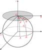 |
Fig. 1 Illustration of the proper distance dP and transverse comoving distance dM in a closed universe (ΩK< 0). The source is AB, and observer is at O. It is obvious that the transverse comoving distance dM is shorter than the proper distance dP. In a flat universe, they are the same, however. The cosmic curvature can therefore be tested by comparing dP and dM. |
Whether our Universe is entirely flat is still unknown, although the latest constraint on the cosmic curvature | ΩK | is less than 0.005 (Planck Collaboration XIII 2016). However, we must keep in mind that this constraint is model dependent, since it is derived in cold dark matter (CDM) background cosmology (Planck Collaboration XIII 2016; Räsänen et al. 2015; Li et al. 2016). Because of the differences between the proper distance and other distances, three important points encourage us to determine the proper distance dP. The first point is that the proper distance dP is the fundamental distance in the Universe. The second point is that the proper distance dP can be used to constrain the cosmic curvature (Yu & Wang 2016). The third point is to test the cosmological principle, that is, the Universe is homogeneous and isotropic at large scales. The basis of this idea is explained in Fig. 1. The transverse distance and proper distance of AB can be regarded as the lengths of the line OB′ and arc OB, respectively. The ratios of the different parts of OB′ and OB can be used to test whether the curvatures at different scales of the Universe are the same. In addition, the cosmological principle is expected to be valid in the proper distance space rather than in dA, dL , or dM space if our Universe is not entirely flat. Therefore we should test the cosmological principle in proper distance space unless we can ensure that our Universe is entirely flat. With a similar idea, Räsänen et al. (2015) tested the FLRW metric using the distance sum rule method (Räsänen et al. 2015). However, the current constraint obtained from this method is very loose.
In order to measure the proper distance, a probe should in principle satisfy two conditions. First, it should change with redshift in a well-understood way and be independent of cosmic curvature. Second, it should record the information on the expansion of our Universe. Standard candles and standard rulers are not able to measure dP since they depend on cosmic curvature. Up to now, no practical method to measure the proper distance has been found. Fortunately, the discovery of fast radio bursts (FRBs; Lorimer et al. 2007; Thornton et al. 2013) and their redshifts (Chatterjee et al. 2017; Tendulkar et al. 2017) sheds light on deriving the proper distance-redshift relation. A radio signal traveling through plasma exhibits a quadratic shift in its arrival time as a function of frequency, which is known as the dispersion measure (DM). The DM of radio signal is proportional to the integrated column density of free electrons along the line of sight (i.e.,  ), which was widely used in Galactic pulsar data (Taylor & Cordes 1993; Manchester et al. 2005) and gamma-ray bursts (Ioka 2003; Inoue 2004). In addition, the redshift measurement of the source gives information on the expansion of the Universe. For an FRB, the DM can be measured directly (Lorimer et al. 2007; Thornton et al. 2013), which has been proposed for cosmological purposes (Zhou et al. 2014; Gao et al. 2014; Lorimer 2016). Its redshift can be estimated by observing its host galaxy or afterglow (Lorimer 2016; Tendulkar et al. 2017). Therefore, the dP − z relation can be derived with the DM and redshift measurements of a large FRB sample.
This paper is organized as follows. In Sect. 2 we introduce the method used to determine the dP − z relation. In Sect. 3 we use Monte Carlo simulations to test the validity and efficiency of our method. We summarize our result in Sect. 4.
2. Method for determining the dP – z relation
2.1. Main idea
FRBs are millisecond-duration radio signals occurring at cosmological distances (Tendulkar et al. 2017). The DM of FRB caused by the intergalactic medium (IGM) is  (4)where
  Ωb is the baryon mass density fraction of the universe, G is the gravitational constant, mp is the rest mass of protons, fIGM is the fraction of baryon mass in the intergalactic medium (IGM),
  represents the average count of electrons contributed by each baryon, YH = 3 / 4 and YHe = 1 / 4 are the mass fractions of hydrogen and helium, and Xe,H and Xe,He are the ionization fractions of intergalactic hydrogen and helium, respectively. The parameters in F(z) are extensively investigated in previous works (Fan et al. 2006; McQuinn et al. 2009; Meiksin 2009; Becker et al. 2011). According to their results, intergalactic hydrogen and helium are fully ionized at z< 3. Therefore we chose Xe,H = Xe,He = 1 at z< 3, which corresponds to fe = 0.875. The values of fIGM are 0.82 and 0.9 at z< 0.4 and z> 1.5, respectively (Meiksin 2009; Shull et al. 2012). To describe the slow evolving of fIGM in the range 0.4 <z< 1.5, we assumed that it increases linearly at 0.4 <z< 1.5 (Zhou et al. 2014). If FRBs can be detected in a wide range of redshifts, we can therefore use the observed DMIGM − z relation to determine the dP − z relation by removing the effect of F(z).
When an FRB signal travels through the plasma from the source to the observer, its DM can be measured with high accuracy. However, this DMobs includes several components that are caused by the plasma in the IGM, the Milky Way, the host galaxy of the FRB, and even the source itself. It has  (5)Only the DMIGM contains the information of the proper distance. Other components therefore need to be subtracted from the DMobs. Since the DMMW is well understood through pulsar data (Taylor & Cordes 1993; Manchester et al. 2005), it can be subtracted. Alternatively, we can only use those FRBs at high galactic latitude that have low DMMW (Zhou et al. 2014; Gao et al. 2014). For the local DMloc, which contains the DMhost and DMsource, the recent finding of the host galaxy of the repeating FRB 121102 suggests a low value ≲324 pc cm-3 and it is probably even lower depending on geometrical factors (Tendulkar et al. 2017). The variation in total DM for FRB 121102 is very small (Spitler et al. 2016; Chatterjee et al. 2017), which indicates that the DMloc is almost constant. Moreover, Yang & Zhang (2016) proposed a method to determine it based on the assumption that DMloc does not evolve with redshift. More fortunately, the DMloc should be decreased by dividing a 1 + z factor since the cosmological time delay and frequency shift. While DMIGM increases with redshift, DMloc is not important at high redshifts. Therefore we can subtract the DMloc from DMobs and leave its uncertainty into the total uncertainty σtot which is the uncertainty of DMIGM extracted from DMobs. It has
  (6)Since the accurate measurement of DM and the well-understood measurement of DMGW, σobs, and σMW can be omitted compared with the much larger σDMloc and σDMIGM. Following Thornton et al. (2013) and numerical simulations of McQuinn (2014), we chose σDMloc = 100 pc / cm3 and σDMIGM = 200 pc / cm3 in the following analysis. These uncertainties are nuisance parameters in an analysis. Fortunately, they can be decreased by using the average DMIGM when there are tens of FRBs in a narrow redshift bin (Zhou et al. 2014; for example, Δz ~ 0.06).
Recently, the host galaxy of FRB 121102 was identified, which can give accurate redshift information (Chatterjee et al. 2017; Tendulkar et al. 2017). When enough FRBs with redshifts are observed, the dP − z relation can be derived from the DMIGM − z relation. Based on the high FRB rate 104 sky-1 day-1 (Thornton et al. 2013), a large sample of FRBs may be collected in the future, which will become the basis of FRB cosmology.
The DMIGM contains the dP information and mixes it with F(z), which corresponds to the anisotropic distribution of free electrons in the Universe. When the effect of F(z) is removed, the dP − z relation can be derived from the DMIGM − z relation. The first step therefore is to reconstruct the DMIGM(z) function of the FRB. The Gaussian process (GP) is a model-independent method to solve this type of problem. The advantage of the GP is that it can reconstruct a function from data without assuming any function form (for more details about the GP, see the next subsection and Rasmussen & Williams 2006). With the GP method, we can therefore obtain the DMIGM − z relation from FRB observational data without any cosmological model assumption. Then we remove the effect of F(z) to obtain the model-independent dP − z relation. In this work, we used the python code package GaPP developed by Seikel et al. (2012). GaPP can reconstruct the function of given data as well as its first, second, and third derivative functions (see Seikel et al. 2012 for more details about GaPP).
With the data set (z, DMobs) of a future sample of observed FRBs, we can use the steps as follows to derive the dP(z).
-
Subtracting the DMMW and DMloc to obtain the data set (z, DMIGM).
-
Dividing the data set (z, DMIGM) into several redshift bins, each of which contains tens of FRBs, and then calculating the average redshift and DMIGM and the standard deviation of DMIGM. Then we have a data set ⟨ z ⟩, ⟨ DMIGM ⟩, and σ⟨ DMIGM ⟩.
-
Using the GP method to reconstruct the function DMIGM(z) and its first derivative function G(z) = dDMIGM(z) / dz.
-
Reintegrating the function
 , which should be c/H(z), to obtain dP(z), where
  , and
, and  can be given by other observations.
2.2. Gaussian process
The GP is a statistical model to smooth a continued function from discrete data. In this model, the value of the function f(x) at any point x is assumed to be a random variable with normal distribution. The mean and Gaussian error value, μ(x) and σ(x), are determined by all of the observed data through a covariance function (or kernel function)  ,
,  and
and  , where
  s are the points with observed data and s are their errors. It has
  (7)and
  (8)When the kernel function is given, we can use the GP to derive the distribution of the continued function f(x).
As we described above, we used the open-source Python package Gapp to apply the GP. This code is widely used (Cai et al. 2016; Yu & Wang 2016). The kernel function in this code is  (9)where σf and l are two parameters to describe the amplitude and length of the correlation in the function value and x directions, respectively. These two parameters can be optimized by the GP with the observational data
  through maximizing their log marginal likelihood function (Seikel et al. 2012),
 ![\begin{eqnarray} \label{likelihood} \ln{\mathcal{L}} &=& \ln{p(f(\tilde{x})|\tilde{x},\sigma_f,l)} \\[3mm] \nonumber &=& -\frac{1}{2}(f(\tilde{x})-\mu(\tilde{x}))^T[K(\tilde{x},\tilde{x})+\sigma_{\tilde{x}}^2I]^{-1}(f(\tilde{x})-\mu{\tilde{x}})\\[3mm] \nonumber &&- \frac{1}{2}\ln{|K(\tilde{x},\tilde{x})+\sigma_{\tilde{x}}^2I|}-\frac{N}{2}\ln{2\pi,} \end{eqnarray}](/articles/aa/full_html/2017/10/aa31607-17/aa31607-17-eq115.png) (10)where N is the number of observed data. In the Gapp package, all of this can be calculated automatically.
(10)where N is the number of observed data. In the Gapp package, all of this can be calculated automatically.
3. Simulations and results
We tested the efficiency of our method using Monte Carlo simulations. First we used Eqs. (4) and (6) to create a mock data set (z, DMIGM, σtot) under a background cosmology. Then we used the above method to derive the dP(z) function and compare it with theoretical dP(z). A flat ΛCDM cosmology with parameters Ωb = 0.049, Ωm = 0.308, ΩΛ = 1 − Ωm, and H0 = 67.8 km s-1 Mpc-1 was assumed (Planck Collaboration XIII 2016). The redshift distribution of the FRBs was assumed as f(z) ∝ ze− z in the redshift range 0 <z< 3, which is similar as the redshift distribution of long gamma-ray bursts (Zhou et al. 2014; Shao et al. 2011). In order to avoid random uncertainty, we simulated 104 times. In each simulation are 500 mock DMIGM, which are equally separated into 50 bins in redshift space.
Figures 2 and 3 show an example of 104 simulations in the ΩK = 0 case. The top panel of Fig. 2 shows the binned DMIGM data (green dots), the reconstructed DMIGM(z) function derived with the GP method (red line), and the theoretical function (blue line). The bottom panel gives the derived and theoretical function G(z). Similar as Fig. 2, Fig. 3 shows the derived and theoretical I(z) and dP(z) function. These figures show that the reconstructed DMIGM(z) function and the final derived dP(z) function are well consistent with theoretical functions, although the G(z) and I(z) functions in middle steps are slightly biased. This shows that the dP(z) function derived from mock DMIGM data with the GP method is reliable.
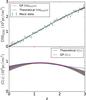 |
Fig. 2 Top panel: binned mock DMIGM data with 1σ errors, the GP reconstructed DMIGM(z) function with its 1σ confidence region, and its theoretical function. Bottom panel: G(z) function with its 1σ confidence region derived from the GP method and its theoretical function. ΩK = 0 is assumed. |
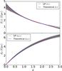 |
Fig. 3 Top panel: I(z) function with its 1σ confidence region derived from the GP method and its theoretical function. Bottom panel: same as the top panel, but for the derived dP(z) function. ΩK = 0 is assumed. |
We also tested the validity and efficiency of our method using the equation 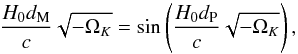 (11)which can constrain ΩK independently of the cosmological model (Yu & Wang 2016). First, 20 mock transverse comoving distance dM data were uniformly simulated from Eq. (3) in the redshift range 1.0 <z< 3.0. Then we performed the same simulations as introduced above in three different fiducial ΩK cases, −0.1, 0, and 0.1. Next, we compared the simulated dM data with the dP(z) function derived with the GP method and used Eq. (11) to solve ΩK. Finally, we took the average value of them and compared it with the fiducial value. To avoid the randomness of simulation, we also simulated this 104 times for each case and drew the posterior probability distributions of the mean ΩK. The top panel of the Fig. 4 shows the posterior probability distributions of ΩK in three different fiducial ΩK cases, −0.1, 0, and 0.1. The assumed cosmic curvatures can be well recovered with errors σ ≈ 0.05 using 500 FRBs data, which also means that the dP(z) function derived from mock DMIGM data with the GP method is reliable and can be used to constrain the cosmic curvature. The bottom two panels show that the errors will decrease to σ ≈ 0.034 and 0.025 when the FRB sample contains 1000 and 2000 FRBs, respectively (the blue histograms in the bottom panels of Fig. 4).
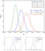 |
Fig. 4 Top panel: posterior distributions of ΩK in three different ΩK cases with 500 mock FRBs data. The derived ΩK value are clearly well consistent with the assumed values. The bottom two panels show the ability of our method when the sample includes 1000 and 2000 FRBs. The blue and green histograms show the results without and with the systematic uncertainty, respectively. |
When deriving the function dP(z), it must be noted that the prior of  with h0 = H0/ 100 km s-1 Mpc-1, and the function F(z) in Eq. (4) will introduce some uncertainties into the derived dP(z) function. For the F(z) function, which describes the distribution of free electrons in the Universe, we can include its contribution to the σDMIGM. We chose σDMIGM = 200 pc / cm3 here, which includes the potential effects of the uncertainty of the function F(z). The more important and nuisance point is the systematic uncertainty caused by the choice of the prior of . From the expression of I(z), it is easy to find that the value of will directly affect the derived dP(z). In order to evaluate the effect of , we considered a Gaussian uncertainty for and repeated the Monte Carlo simulations. Since the uncertainty of is about 1% (Planck Collaboration XIII 2016), we chose the value of the systematic uncertainty as 1%. The results are shown as the green histograms in the bottom panels of Fig. 4. For 1000 FRBs with redshift measurements, the uncertainty of the ΩK is about 0.05, which is acceptable. However, the exact value of H0 is still unknown. For the value of H0, the value from Cepheid+SNe Ia and the cosmic microwave background (CMB) differs. For example, Riess et al. (2016) derived the best estimate of H0 = 73.24 ± 1.74 km s-1 Mpc-1 using Cepheids, which is about 3.4σ higher than the value from Planck Collaboration XIII (2016). However, Aubourg et al. (2015) used the 2013 Planck data in combination with BAO and the JLA SNe data to find H0 = 67.3 ± 1.1 km s-1 Mpc-1, in excellent agreement with the 2015 Planck value. Moreover, H0 = 62.3 ± 6.3 km s-1 Mpc-1 is derived from the Cepheid-calibrated luminosity of SNe Ia (Sandage et al. 2006), which agrees with the 2015 Planck value. Therefore we used the best constraint on from Planck CMB data.
The systematic uncertainty is always a nuisance problem in all cosmology probes, such as SNe Ia as the probe of the luminosity distances and BAO as the probe of the angular diameter distances. SNe Ia are widely accepted to be excellent standard candles at optical wavelengths. The luminosity distances could be derived from SNe Ia. However, the exact nature of the binary progenitor system (a single white dwarf accreting mass from a companion, or the merger of two white dwarfs) still is an open question. Systematic errors, including calibration, Malmquist bias, K-correction, and dust extinction, degrade the quality of SNe Ia as standard candles (Riess et al. 2004). Moreover, the derived luminosity distances are not fully model independent (Suzuki et al. 2012). The derived cosmological parameters from SNe Ia are significantly biased by systematic errors (see Fig. 5 of Suzuki et al. 2012, for details). The angular diameter distances for galaxy clusters can be obtained by combining the Sunyaev-Zeldovich temperature decrements and X-ray surface brightness observations. The error of the angular diameter distance can be up to 20% (Bonamente et al. 2006), however. Therefore the dP(z) derived from FRBs can be a supplementary tool, although greater efforts are required on its systematic error.
4. Summary
In cosmology, the proper distance dP corresponds to the length of the light path between two objects. It is a potentially useful tool to test the cosmic curvature and cosmological principle. In the past, the proper distance was seldom used to investigate our Universe since it is difficult to measure. We proposed a model-independent method to derive the proper distance-redshift relation dP(z) from DM and redshift measurements of FRBs. The basis of our method is that many FRBs with measured redshifts and DMs may be observed in a wide redshift range (i.e., 0 <z< 3) in the future. This is possible because of the high rate of FRBs, which is about 104 sky-1 day-1 (Thornton et al. 2013). Although some authors have used FRBs as cosmological probes (Zhou et al. 2014; Gao et al. 2014), they only considered DMs. The most important point is that the distance information contained in DMs is the proper distance dP, whose difference with other distances is important in understanding the fundamental properties of our Universe.
In the near future, several facilities such as the Canadian Hydrogen Intensity Mapping Experiment (CHIME) radio telescope, the Five-hundred-meter Aperture Spherical Telescope (FAST) in China, and the Square Kilometer Array will commence working. Interestingly, the CHIME might detect dozens of FRBs per day (Kaspi 2016). A large sample of FRBs with redshift measurements is therefore expected in next decade (Lorimer 2016). With a large sample of FRBs, the proper distance derived from FRBs will be a new powerful cosmological probe.
Acknowledgments
We thank the anonymous referee for constructive comments. This work is supported by the National Basic Research Program of China (973 Program, grant No. 2014CB845800), the National Natural Science Foundation of China (grants 11422325 and 11373022), the Excellent Youth Foundation of Jiangsu Province (BK20140016). H. Yu is also supported by the Nanjing University Innovation and Creative Program for PhD candidates (2016012).
References
- Becker, G. D., Bolton, J. S., Haehnelt, M. G., & Sargent, W. L. W. 2011, MNRAS, 410, 1096 [NASA ADS] [CrossRef] [Google Scholar]
- Bonamente, M., Joy, M. K., LaRoque, S. J., et al. 2006, ApJ, 647, 25 [NASA ADS] [CrossRef] [Google Scholar]
- Cai, R.-G., Guo, Z.-K., Yang, T. 2016, Phys. Rev. D, 93, 043517 [NASA ADS] [CrossRef] [Google Scholar]
- Chatterjee, S., Law, C. J., Wharton, R. S., et al. 2017, Nature, 541, 58 [NASA ADS] [CrossRef] [Google Scholar]
- Coles, P., & Lucchin, F. 2002, Cosmology: The origin and Evolution of Cosmic Structure (Wiley-VCH) [Google Scholar]
- Eisenstein, D. J., Zehavi, I., Hogg, D. W., et al. 2005, ApJ, 633, 560 [NASA ADS] [CrossRef] [Google Scholar]
- Fan, X., Carilli, C. L., Keating, B. 2006, ARA&A, 44, 415 [NASA ADS] [CrossRef] [Google Scholar]
- Gao, H., Li, Z., & Zhang, B. 2014, ApJ, 788, 189 [NASA ADS] [CrossRef] [Google Scholar]
- Hogg, D. W. 1999, ArXiv e-prints [arXiv:astro-ph/9905116] [Google Scholar]
- Inoue, S. 2004, MNRAS, 348, 999 [NASA ADS] [CrossRef] [Google Scholar]
- Ioka, K. 2003, ApJ, 598, L79 [NASA ADS] [CrossRef] [Google Scholar]
- Kaspi, V. M. 2016, Science, 354, 1230 [NASA ADS] [CrossRef] [Google Scholar]
- Li, Z., Wang, G.-J., Liao, K., & Zhu, Z.-H. 2016, ApJ, 833, 240 [NASA ADS] [CrossRef] [Google Scholar]
- Lorimer, D. 2016, Nature, 530, 427 [NASA ADS] [CrossRef] [Google Scholar]
- Lorimer, D. R., Bailes, M., McLaughlin, M. A., Narkevic, D. J., & Crawford, F. 2007, Science, 318, 777 [NASA ADS] [CrossRef] [PubMed] [Google Scholar]
- Manchester, R. N., Hobbs, G. B., Teoh, A., & Hobbs, M. 2005, AJ, 129, 1993 [NASA ADS] [CrossRef] [Google Scholar]
- McQuinn, M. 2014, ApJ, 780, L33 [NASA ADS] [CrossRef] [Google Scholar]
- McQuinn, M., Lidz, A., Zaldarriaga, M., et al. 2009, ApJ, 694, 842 [NASA ADS] [CrossRef] [Google Scholar]
- Meiksin, A. A. 2009, Rev. Mod. Phys., 81, 1405 [NASA ADS] [CrossRef] [Google Scholar]
- Perlmutter, S., Perlmutter, S., Aldering, G., Goldhaber, G., et al. 1999, ApJ, 517, 565 [NASA ADS] [CrossRef] [Google Scholar]
- Planck Collaboration XIII. 2016, A&A, 594, A13 [NASA ADS] [CrossRef] [EDP Sciences] [Google Scholar]
- Räsänen, S., Bolejko, K., Finoguenov, A. 2015, Phys. Rev. Lett., 115, 101301 [NASA ADS] [CrossRef] [Google Scholar]
- Rasmussen, C., & Williams, C. 2006, Gaussian Processes for Machine Learning (Cambridge: MIT Press) [Google Scholar]
- Riess, A. G., Filippenko, A. V., Challis, P., et al. 1998, AJ, 116, 1009 [NASA ADS] [CrossRef] [Google Scholar]
- Riess, A. G., Strolger, L.-G., Tonry, J., et al. 2004, ApJ, 607, 665 [NASA ADS] [CrossRef] [Google Scholar]
- Sandage, A., Tammann, G. A., Saha, A., et al. 2006, ApJ, 653, 843 [NASA ADS] [CrossRef] [Google Scholar]
- Seikel, M., Clarkson, C., Smith, M. 2012, J. Cosmol. Astro-Particle Phys., 6, 036 [Google Scholar]
- Shao, L., Dai, Z.-G., Fan, Y.-Z., et al. 2011, ApJ, 738, 19 [NASA ADS] [CrossRef] [Google Scholar]
- Shull, J. M., Smith, B. D. & Danforth, C. W. 2012, ApJ, 759, 23 [NASA ADS] [CrossRef] [Google Scholar]
- Spitler, L. G., Scholz, P., Hessels, J. W. T., et al. 2016, Nature, 531, 202 [NASA ADS] [CrossRef] [Google Scholar]
- Suzuki, K., Nagai, H., Kino, M., et al. 2012, ApJ, 746, 140 [NASA ADS] [CrossRef] [Google Scholar]
- Taylor, J. H., & Cordes, J. M. 1993, ApJ, 411, 674 [NASA ADS] [CrossRef] [Google Scholar]
- Tendulkar, S. P., Bassa, C. G., Cordes, J. M., et al. 2017, ApJ, 834, L7 [NASA ADS] [CrossRef] [Google Scholar]
- Thornton, D., Stappers, B., Bailes, M., et al. 2013, Science, 341, 53 [NASA ADS] [CrossRef] [PubMed] [Google Scholar]
- Wang, F. Y., Dai, Z. G., & Liang, E. W. 2015, New Astron. Rev., 67, 1 [NASA ADS] [CrossRef] [Google Scholar]
- Weinberg, D. H., Mortonson, M. J., Eisenstein, D. J., et al. 2013, Phys. Rev., 530, 87 [Google Scholar]
- Weinberg, S. 1972, Gravitation and Cosmology: Principles and Applications of the General Theory of Relativity (Wiley-VCH) [Google Scholar]
- Yang, Y.-P., Zhang, B. 2016, ApJ, 830, L31 [NASA ADS] [CrossRef] [Google Scholar]
- Yu, H., & Wang, F. Y. 2016, ApJ, 828, 85 [NASA ADS] [CrossRef] [Google Scholar]
- Zhou, B., Li, X., Wang, T., Fan, Y.-Z., & Wei, D.-M. 2014, Phys. Rev. D, 89, 107303 [NASA ADS] [CrossRef] [Google Scholar]
All Figures
|
Fig. 1 Illustration of the proper distance dP and transverse comoving distance dM in a closed universe (ΩK< 0). The source is AB, and observer is at O. It is obvious that the transverse comoving distance dM is shorter than the proper distance dP. In a flat universe, they are the same, however. The cosmic curvature can therefore be tested by comparing dP and dM. |
| In the text | |
|
Fig. 2 Top panel: binned mock DMIGM data with 1σ errors, the GP reconstructed DMIGM(z) function with its 1σ confidence region, and its theoretical function. Bottom panel: G(z) function with its 1σ confidence region derived from the GP method and its theoretical function. ΩK = 0 is assumed. |
| In the text | |
|
Fig. 3 Top panel: I(z) function with its 1σ confidence region derived from the GP method and its theoretical function. Bottom panel: same as the top panel, but for the derived dP(z) function. ΩK = 0 is assumed. |
| In the text | |
|
Fig. 4 Top panel: posterior distributions of ΩK in three different ΩK cases with 500 mock FRBs data. The derived ΩK value are clearly well consistent with the assumed values. The bottom two panels show the ability of our method when the sample includes 1000 and 2000 FRBs. The blue and green histograms show the results without and with the systematic uncertainty, respectively. |
| In the text | |
Current usage metrics show cumulative count of Article Views (full-text article views including HTML views, PDF and ePub downloads, according to the available data) and Abstracts Views on Vision4Press platform.
Data correspond to usage on the plateform after 2015. The current usage metrics is available 48-96 hours after online publication and is updated daily on week days.
Initial download of the metrics may take a while.