| Issue |
A&A
Volume 606, October 2017
|
|
|---|---|---|
| Article Number | A82 | |
| Number of page(s) | 25 | |
| Section | Interstellar and circumstellar matter | |
| DOI | https://doi.org/10.1051/0004-6361/201731262 | |
| Published online | 16 October 2017 | |
The observed chemical structure of L1544 ⋆,⋆⋆
Max Planck Institute for Extraterrestrial Physics, Giessenbachstrasse 1, 85748 Garching, Germany
e-mail: spezzano@mpe.mpg.de
Received: 29 May 2017
Accepted: 18 July 2017
Context. Prior to star formation, pre-stellar cores accumulate matter towards the centre. As a consequence, their central density increases while the temperature decreases. Understanding the evolution of the chemistry and physics in this early phase is crucial to study the processes governing the formation of a star.
Aims. We aim to study the chemical differentiation of a prototypical pre-stellar core, L1544, by detailed molecular maps. In contrast with single-pointing observations, we performed a deep study on the dependencies of chemistry on physical and external conditions.
Methods. Here we present the emission maps of 39 different molecular transitions belonging to 22 different molecules in the central 6.25 arcmin2 of L1544. We classified our sample into five families, depending on the location of their emission peaks within the core. To systematically study the correlations among different molecules, we have performed the principal component analysis (PCA) on the integrated emission maps. The PCA allows us to reduce the amount of variables in our dataset. Finally, we have compared the maps of the first three principal components with the H2 column density map, and the Tdust map of the core.
Results. The results of our qualitative analysis is the classification of the molecules in our dataset in the following groups: (i) the c-C3H2 family (carbon chain molecules like C3H and CCS); (ii) the dust peak family (nitrogen-bearing species like N2H+); (iii) the methanol peak family (oxygen-bearing molecules like methanol, SO and SO2); (iv) the HNCO peak family (HNCO, propyne and its deuterated isotopologues). Only HC18O+ and 13CS do not belong in any of the above mentioned groups. The principal component maps allow us to confirm the (anti-)correlations among different families that were described in a first qualitative analysis, but also point out the correlation that could not be inferred before. For example, the molecules belonging to the dust peak and the HNCO peak families correlate in the third principal component map, hinting on a chemical and/or physical correlation.
Conclusions. The principal component analysis has shown to be a powerful tool to retrieve information about the correlation of different molecular species in L1544, and their dependence on physical parameters previously studied in the core.
Key words: ISM: clouds / ISM: molecules / radio lines: ISM / ISM: individual objects: L1544
Based on observations carried out with the IRAM 30 m telescope. IRAM is supported by INSU/CNRS (France), MPG (Germany) and IGN (Spain).
The integrated emission maps for each line (FITS files) are only available at the CDS via anonymous ftp to cdsarc.u-strasbg.fr (130.79.128.5) or via http://cdsarc.u-strasbg.fr/viz-bin/qcat?J/A+A/606/A82
© ESO, 2017
1. Introduction
Starless cores represent the earliest phase of star formation. At this stage the protostar is not yet formed, so it is possible to study the chemistry and physics independently of the complexity arising from the proto-stellar feedback. Pre-stellar cores are starless cores on the verge of star formation, the central density of H2 is higher than 105 cm-3 and therefore they are thermally supercritical (Keto & Caselli 2008). L1544 is a well-studied pre-stellar core in Taurus. It is centrally concentrated (Ward-Thompson et al. 1999), relatively massive (Tafalla et al. 1998), it shows very high deuteration (Crapsi et al. 2005), and radiative transfer studies show that it is contracting in a quasi-static fashion (Keto & Caselli 2008, 2010; Keto et al. 2015). While several single pointing observations have been performed to study the chemistry of L1544, fewer maps are available. N2H+ and CCS are the first molecules that have been mapped towards L1554 (Williams et al. 1999; Ohashi et al. 1999), and a chemical inhomogeneity of the core has already been suggested. CCS is less abundant towards the dust peak, while N2H+ suffers less the depletion caused by the high density and low temperature. The lack of substantial depletion for N2H+ has been confirmed by several studies: Caselli et al. (2002) for instance show that N2D+, even better than N2H+, traces the inner region of L1544, close to the dust peak (Ward-Thompson et al. 1999). Bergin et al. (2002) found hints of depletion of N2H+ towards the centre of B68. The molecular differentiation in L1544 and other starless cores was furthermore studied by Tafalla et al. (2002) by mapping CO and CS isotopologues, NH3 and N2H+. All the cores, including L1544, show an abundance drop of CO and CS at the dust peak, a constant N2H+ abundance and an increase of NH3 towards the centre. While the behaviour of CO, CS and N2H+ are explained by depletion models, the increase of ammonia towards the centre is not yet well understood (Caselli et al. 2017). The maps of DNC and HN13C in L1544 and other starless cores show that, unlike the ratio N[DCO+]/N[HCO+], the column density ratio N[DNC]/N[HNC] is not sensitive to the depletion factor (Hirota et al. 2003). The peculiar absence of depletion of nitrogen-bearing species has been used by Crapsi et al. (2007) to study the thermal structure of the denser parts in L1544 by mapping NH3 and NH2D. Recently it has been pointed out that the chemical differentiation in L1544 is not limited to nitrogen- and carbon-bearing species. Carbon-bearing molecules further differentiate, and in particular methanol (CH3OH) and cyclopropenylidene (c-C3H2) present a complementary morphology (Spezzano et al. 2016b).
This paper is an extensive study on the chemical differentiation in L1544. Maps of over 30 species are presented, and their different spatial distributions are discussed. The analysis will be carried out using the principal component analysis (PCA). This method has been successfully applied in other multi-line studies of other regions of our Galaxy, such as Orion (Ungerechts et al. 1997; Gratier et al. 2017) and supernova remnants (Neufeld et al. 2007). In Gratier et al. (2017), for example, the PCA has been used to study the correlation between the emission maps of 12 molecular lines in the south-western edge of Orion B giant molecular cloud over a field of view of 1.5 square degrees.
The paper is structured as follows: the observations are described in Sect. 2, a first qualitative analysis of the data is presented in Sect. 3, and the results of the multivariate analysis are described in Sect. 4. In Sect. 5 we summarise our results and conclusions.
Spectroscopic parameters of the observed lines, divided depending on the position of their emission peaks.
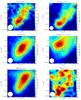 |
Fig. 1 Sample of maps belonging to the different families observed towards L1544. The full dataset is shown in Appendix A. The black dashed lines represent the 90%, 50%, and 30% of the H2 column density peak value derived from Herschel maps (Spezzano et al. 2016b), 2.8 × 1022 cm-2. The solid lines represent contours of the molecular integrated emission starting with 3σ with steps of 3σ (the rms of each map is reported in Table 1). The dust peak (Ward-Thompson et al. 1999) is indicated by the black triangle. The white circles represent the HPBW of the 30 m telescope. |
2. Observations
The emission maps towards L1544 were obtained using the IRAM 30 m telescope (Pico Veleta, Spain) in three different observing runs in October 2013, July 2015, and January 2017, and are shown in Figs. A.1–A.5. A sample of the observed maps is presented in Fig. 1. We performed a 2.5′ × 2.5′ on-the-fly (OTF) map centred on the source dust emission peak (α2000 = 05h04m17 21, δ2000 = +25°10′42
 8). Position switching was used, with the reference position set at (−180′′, 180′′) offset with respect to the map centre. The observed transitions are summarised in Table 1. The EMIR E090 receiver was used with the Fourier transform spectrometer backend (FTS) with a spectral resolution of 50 kHz. The antenna moved along an orthogonal pattern of linear paths separated by 8′′ intervals, corresponding to roughly one third of the beam full width at half maximum (FWHM). The mapping was carried out in good weather conditions (τ ~ 0.03) and a typical system temperature of Tsys ~ 90–100 K. The data processing was done using the GILDAS software (Pety 2005) and CASA (McMullin et al. 2007). All the emission maps presented in this paper have been gridded to a pixel size of 4′′ with the CLASS software in the GILDAS package, this corresponds to 1/5–1/7 of the actual beam size, depending on the frequency. The integrated intensities have been calculated in the 6.7–7.7 km s-1 velocity range.
3. Results and discussion
By making a qualitative comparison of their distributions in L1544, we can classify our sample of molecules in five different families: those with integrated intensity maps peaking nearby the (i) c-C3H2 peak (c-C3H2 and C4H in Fig. 1); (ii) dust peak (H13CN in Fig. 1); (iii) methanol peak (CH3OH in Fig. 1); (iv) HNCO peak (HNCO in Fig. 1). Only a few do not belong to the above groups (13CS in Fig. 1). Figure 1 shows some of the molecules presenting different spatial distribution within L1544, the whole observed sample is reported in Figs. A.1–A.5.
3.1. c-C3H2 peak
The molecules belonging to this category peak towards the south-east of the core, see the maps in Fig. A.1. As already discussed in Spezzano et al. (2016b), this spot corresponds to a sharp edge in the H2 column density map and hence it is more affected by the interstellar radiation field (ISRF). The carbon-chain chemistry (CCC) is enhanced and as a consequence, C-rich molecules have their emission peak in this region. Indeed the molecules that we find being abundant in the c-C3H2 peak are: H2CCC, C3H, C4H, H2CCO, HCCNC, H2CS, HCS+, C34S, CCS, CH3CN, HCC13CN and of course c-C3H2 and its 13C isotopologue c-H13CC2H. We note that only sulphur molecules containing carbon are present here. This could be due to the presence of S+, which can readily react with hydrocarbons (Smith et al. 1988).
3.2. Dust peak
The molecules that are more abundant towards the dust peak are nitrogen-containing molecules: H13CN, 13CN and N2H+, see Fig. A.2. It has long been known that nitrogen-bearing molecules suffer less depletion towards the dust peak of starless cores with respect to other molecules, CO for example (Caselli et al. 1999). This is evident from our maps as well. While all the other molecules, no matter where they peak, avoid the central denser region of L1544, nitrogen-bearing molecules are more abundant towards the dust peak. The explanation for such behaviour is not yet clear. Laboratory studies show that the desorption rates and sticking probabilities of N2 and CO are very similar (Bisschop et al. 2006), but the observations in L1544 and other starless cores show that CO depletes at higher temperatures and lower densities than N2H+. A possible explanation for this is that CO at least partially destroys N2H+ (producing HCO+), so that N2H+ thrives when CO starts to freeze out (e.g. Aikawa et al. 2001). Moreover, N2 formation may still be ongoing in the gas phase when CO becomes heavily depleted (e.g. Flower et al. 2006).
3.3. Methanol peak
Bizzocchi et al. (2014) presented the first map of methanol towards L1544, showing a clear peak towards the north of the dust continuum peak. We have recently pointed out that the methanol distribution differs from that of cyclopropenylidene, c-C3H2 (Spezzano et al. 2016b). This leads to a not-yet-understood spatial differentiation within C-bearing molecules. Here we present the maps of several molecules peaking at the methanol peak: SO, 34SO, SO2, OCS and methanol, see Fig. A.3. Three hyperfine components of HCO are also present in our data, but the achieved signal-to-noise ratio allows us to map only the NKa,Kc = 10,1–00,0J = 3/2–1/2 F = 2–1 transition. Despite many of the molecules that peak in this position contain sulphur, we do not believe that sulphur chemistry plays a crucial role in the chemical differentiation that we observe. In fact, the sulphur-bearing species that are carbon-based are more abundant towards the c-C3H2 peak. The sulphur-bearing molecules here all contain oxygen (unlike those towards the c-C3H2 peak). Jiménez-Serra et al. (2016) show that O-bearing complex molecules (COM) such as methyl formate and dimethyl ether are also more abundant towards the methanol peak while N-bearing COM like HCCNC, CH3CN and CH2CHCN are more abundant towards the dust peak. From our data we can confirm that O-bearing molecules are indeed more abundant in the low-density shell towards the north of L1544, while HCCNC and CH3CN peak towards the south-east like the other C-bearing molecules. The O-bearing molecules deplete towards the dust peak and are less abundant towards the south where the C/O atomic ratio is quite large, because of the photodissociation of CO, and the formation rate of carbon chains is very high (e.g. Herbst & Leung 1989).
3.4. HNCO peak
Four different species have their emission peak in none of the three positions discussed above. These species are CH3CCH, CH2DCCH, CH3CCD, and HNCO, see Fig. A.4. The lines of CH3CCH and HNCO are relatively bright and if their emission is optically thick, the distribution might be affected and hence not representative of the whole core. We should be able to estimate the optical depth based on the upper limit of the 13C isotopologue, assuming a 12C/13C of 77 (Wilson & Rood 1994). Unfortunately we did not detect any lines of the 13C isotopologue of propyne, CH3CCH, so we cannot deduce its spatial distribution from the 13C isotopologue. Instead, we have observed two deuterated isotopologues, CH2DCCH and CH3CCD, and they also peak towards the HNCO peak. Given that we believe it would be quite surprising for a deuterated isotopologue to be optically thick, an additional molecular peak is indeed present in L1544 towards the north-west, and not produced by optical depth effects. Here we refer to it as the HNCO peak. We have also mapped two lines of HNCO, and they both show their emission peak towards the north-west. No 13C isotopologue was observed, so we cannot rule out that the emission peak shown by HNCO is caused by large optical depth by comparing with a rare isotopologue. We have instead used the online RADEX tool, a one-dimensional non-LTE radiative transfer code (van der Tak et al. 2007). We have checked the optical depth of the two observed lines of HNCO by assuming a kinetic temperature ranging from 8 to 12 K and a density from 1 × 10⁵ to 1 × 10⁶ H2 molecules per cubic centimetre and we obtain optical depths in the range of 0.1 to 0.3. As a consequence we can safely assume that the spatial distribution of HNCO is not affected by a large optical depth.
HNCO contains all the atoms present in prebiotic molecules, and its correlation with formamide (NH2CHO) has been discussed in the literature (López-Sepulcre et al. 2015; Barone et al. 2015). If the HNCO peak was a genuine molecular peak in L1544, it would be the best place to look for prebiotic molecules like formamide, and shine some light on the formation of life-seeds in the earliest phases of star formation.
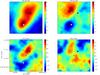 |
Fig. 2 Maps of the first four principal components obtained by performing the PCA on the standardised data. The maps are constructed by summing for each pixel the contribution of each molecular transition scaled by the values reported in Table 2, i.e. they represent each pixel projected in the space of the principal components. The percentages represent the amount of correlation that can be reproduced by the single principal component. The blue, black, white, and grey diamonds indicate the dust, the HNCO, the c-C3H2, and the methanol peaks respectively. |
3.5. Other
Two molecules do not fall in neither of the four categories described above, see Fig. A.5. HC18O+ does not peak towards the c-C3H2 peak, but it is clearly depleted towards the centre of L1544. A similar behaviour was already observed by Caselli et al. (2002) for H13CO+. 13CS shows a clear “doughnut” shape around L1544, indicating very clearly its depletion towards the dust peak, and peaking towards both the c-C3H2- and methanol peak. The map of the J = 2–1 transition of CS, main isotopologue, was reported in Tafalla et al. (2002) and presents a diffuse and fragmented distribution compared to the N2H+ and NH3 maps. Both molecules (CS and HC18O+) are expected to be quite abundant in the molecular cloud within which L1544 is embedded, so their distribution may be affected by the large-scale structure of the cloud.
Eingenvalues and eigenvectors derived from principal component analysis on the standardised data.
4. Multivariate analysis
To make an unbiased study of our large data set and systematically study the correlations among different molecules, we have performed the PCA on integrated emissions in L1544. We have used the PCA implementation available in the Python package “scikit-learn” (Pedregosa et al. 2011). The PCA is a multivariate analysis technique that allows us to reduce the dimensionality of the variables in our data set. It is widely used in natural sciences, and it has also been used to study the physics and chemistry of the ISM (Ungerechts et al. 1997; Neufeld et al. 2007; Lo et al. 2009; Melnick et al. 2011; Jones et al. 2012; Gratier et al. 2017). The PCA method has been extensively described in Ungerechts et al. (1997). Briefly, the principal components (PCs) are derived by finding the eigenvalues and eigenvectors of a covariance (or correlation) matrix, with the eigenvalues being the variance (or correlation) accounted for by each PC, and the eigenvectors the contributions of each molecule to the each PC.
When performing the PCA, we treat our data as 1369 points (37 × 37 pixels in each map), in a space with 28 dimensions (the number of molecular transitions that we use in the analysis). In our analysis we have included one molecular transition for each molecule that we have observed. In the case of molecules that have been mapped in several transitions, we have selected the map with the best signal-to-noise ratio. The molecular transitions included in the PCA are marked with a star in Table 1. In order to reduce the number of variables, we have described the variations in the 28 maps as a superimposition of fewer variables, the principal components. The maps of the PC helped us identify the regions within L1544 with stronger (anti-)correlations among the different molecules. As done in the literature, we standardised the data before performing the PCA, meaning that they are mean-centred and normalised. The standardised value is described as follows:  (1)with μ being the mean value and σ being the standard deviation for each map. The data before and after the standardisation are reported Figs. B.1 and B.3, where a more detailed explanation of the need for preprocessing the data is presented.
The maps have not been convolved to a common angular resolution before performing the PCA. We ran some tests, and find that the effect of convolving all the maps to 29′′ is negligible. In Table 2 we report the results of our principal component analysis: the eigenvalues and eigenvectors of the first four principal components, and Fig. 2 shows the projection of our data onto the PC, that is, the principal component maps. It is mathematically possible to compute up to 28 independent PC, as many as the number of our maps. Figure 2 shows the maps of the first four principal components because for the purpose of our study it is enough to focus on those carrying most of the correlation, and the first four PCs togehter account for more than 85% of the correlation in our dataset.
Figure 3 shows the contribution of each emission line to each of the first four PC. The PC maps have no physical meaning, but they are very useful when compared with physical maps of L1544 to find possible (anti-)correlations among species and with the different physical conditions across the core. Figure 4 shows the eigenvectors of the first four PC plotted as correlation wheels. For the clarity of the plot, only a fraction of the molecules are shown, selected from those showing the most prominent (anti-)correlation features.
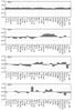 |
Fig. 3 Contribution of each molecular transition to the first four PC, obtained by performing the PCA on the standardised data. |
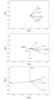 |
Fig. 4 Correlation wheels where each molecule has as coordinates their correlation coefficients to each PC, obtained by performing the PCA on the standardised data. |
The first PC positively correlates with all of the 28 molecular transitions observed, see Table 2. Its map, see Fig. 2, resembles the continuum map of L1544 with the difference that while the latter peaks at the denser part of L1544 (the dust peak shown as a black triangle in the maps in Figs. A.1–A.5), the PC1 map peaks at the c-C3H2 and HNCO peaks. The first PC represents a weighted mean of all lines, in fact the distribution of most of the molecules in our sample (80%) follows the density distribution described by the continuum map. Such a feature has been observed in all previous studies of the ISM with the PCA, for example, Ungerechts et al. (1997). The only exceptions are the molecules that peak towards the methanol peak, of which there are just six in a sample of 28, that is, 20%. In PC1, the dust peak is not as intense as the HNCO peak, even if they both contribute with four molecular transitions to the dataset, because all of the molecules peaking in the c-C3H2 and HNCO peak are depleted towards the centre of the core.
The second PC map clearly represents the two most prominent molecular peaks in L1544, the c-C3H2 peak and the methanol peak. It correlates positively with all of the molecules peaking at the methanol peak, namely SO, SO2, OCS, HCO, and methanol. On the other hand, all the C-chain molecules anti-correlate with the second PC. This differentiation has been already explained in Spezzano et al. (2016b), and it is related to a non-uniform exposure to the ISRF. Towards the south, where the C-chain molecules peak, L1544 presents a sharp edge in the H2 column density, clearly shown in Fig. 1 of Spezzano et al. (2016b). This region is less shielded from the ISRF and hence photochemistry is more prominent, keeping more carbon atoms available to support a rich carbon chemistry. On the contrary, the methanol peak is farther away from the southern edge, hence more protected from the ISRF. Here carbon is mostly locked in CO. It is interesting to see that all of the molecules peaking towards the other two molecular peaks in L1544, the dust- and the HNCO peak, do not contribute substantially to the second PC.
While in the second PC map the difference between two molecular peaks is evident, and confirms our first qualitative classification, the third map brings together the dust and the HNCO peak. All of the molecules peaking in these two positions in fact correlate positively with the third PC. It is not trivial to see a chemical relationship among these molecules. While 13CN and N2H+ are both chemically related to N2, it is less easy to find a common denominator with HNCO and CH3CCH. A closer look into chemical models should help find the link between these four molecules.
By looking at the contributions to the fourth PC, see Fig. 3, we note that there is no common behaviour for the different molecules belonging to the same family. The same happens also for the fifth PC, which is not shown in this paper. Given the amount of the total correlation that the combined fourth and fifth PCs account for (less than 5%), and the fact that we aim to use the PCA to find connections between the different families and physical quantities, we focus our attention only on the first three PCs.
4.1. Effect of noise
As done in Gratier et al. (2017), we evaluated the effect of the noise on our results by performing the PCA on 5000 datasets which were constructed by adding random (Gaussian) noise to the maps, according to the standard deviation of the noise in each single map. We then computed the standard deviation of the PC coefficients for each molecule in the first 20 PC. We evaluated the effect of the noise by comparing the standard deviation of the PC coefficient for each molecule in each PC, with its mean within the 5000 resulting values (σ/μ). We find that the effect on the first three PC is completely negligible (σ/μ< 5%), and it is very small for the fourth and fifth PC (σ/μ< 10%). From the sixth PC on, the effect of the noise is instead relevant (σ/μ ~ 30%).
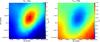 |
Fig. 5 Maps of the H2 column density and the dust temperature in L1544. |
4.2. Correlation with physical maps
As done in Gratier et al. (2017), we computed the Spearman’s rank correlation coefficients between the first three PC maps and the physical maps of L1544. It is important to keep in mind that the physical maps that we present are correlated, while the PC maps are uncorrelated by definition. The physical maps that we have used are shown in Fig. 5 and they are the H2 column density map and the Tdust map. The maps have been derived from Herschel/SPIRE data, following the method described in Spezzano et al. (2016b) where the NH2 map has already been presented. The correlation coefficients are reported in Table 3.
The NH2 map correlates very well with the map of the first principal component. This behaviour has been already reported in previous studies, Gratier et al. (2017) for example, and it reflects the fact that the PC1 map can be interpreted like a global column density map. Given the fact that Tdust anti-correlates with NH2 (high densities correspond to low temperatures), the first principal component shows a negative correlation with respect to them.
All the physical maps show a weak (anti-)correlation to the second principal component. The chemical differentiation described by the PC2 (for example methanol vs. c-C3H2) is in fact the result of large scale effects that are not taken into consideration in the small scale maps used for this analysis. This is very well explained by Fig. 3 in Spezzano et al. (2016b), where the H2 column density presents a steep drop towards the south-west, while the drop is more shallow towards the north-east. For this reason, the gas at the c-C3H2 peak in L1544 is less shielded from the UV illumination than the gas at the methanol peak.
The third PC map, that well correlates with the molecules abundant at the dust and HNCO peak, does not show (anti-)correlation to any of the physical maps. Such a behaviour might be explained by the fact that these two classes of molecules present such spatial distribution because of a peculiar chemistry, or micro-physics properties (such as desorption rates and sticking probabilities) that are not affected by local variations in visual extinction (or NH2) and Tdust.
Spearman’s rank correlation coefficients computed between the physical maps and the first three principal components.
5. Conclusions
We have presented the emission maps of 39 different molecular transitions towards the pre-stellar core L1544. The molecules present in our dataset have been divided in categories based on their spatial distribution. This qualitative approach has allowed us to recognise four molecular peaks in L1544: the c-C3H2 peak, the methanol peak, the dust peak and the HNCO peak. The molecules belonging to the c-C3H2 family are carbon chain molecules: cyclic and linear C3H2, C3H, C4H, H2CCO, H2CS, C34S, CCS, CH3CN and HCC13CN. The molecules belonging to the methanol peak family are characterised by the presence of oxygen: methanol, SO, 34SO, SO2, OCS, and HCO. Molecules chemically related to N2 instead peak towards the dust peak: 13CN, H13CN, and N2H+. The molecules belonging to the HNCO family are HNCO, CH3CCH and its deuterated isotopologues. The chemical and/or physical connection among these molecules is still under investigation. 13CS and HC18O+ have a diffuse distribution within L1544, possibly affected by the large scale structure of the cloud.
In order to take into consideration underlying differences and similarities, we performed the PCA on a selected sample of molecular transitions in our dataset. The results of the PCA have confirmed the correlation among the molecules in the four categories depending on the spatial distribution, especially the dichotomy between the molecules peaking in the methanol and the c-C3H2 peak. The PCA has also shown a correlation between the molecules in the HNCO and the dust peak of L1544, which could not be found just from a qualitative analysis. Further studies on the chemical link between these molecules will help shine some light on their correlation.
We calculated the Spearman’s rank correlation coefficients between the first three PC maps and the maps of H2 column density and the dust temperature in L1544. The first PC map, a weighted mean of all molecular transitions included in the analysis, correlates very well with the H2 column density maps of L1544. The second PC, which reproduces well the contrast between methanol and c-C3H2, instead does not correlate substantially with the physical maps. This is in accordance with the large scale effects due to external illumination that we believe are responsible for the different spatial distributions of these two molecules. The third PC, which correlates with the molecules peaking both in the HNCO and dust peak, also shows no correlation with any of the physical maps, maybe suggesting that the link between these molecules has to be found in their chemistry or in the microphysics involved in the interaction with the ices. A comparison with chemical modelling results will be presented in an upcoming paper (Spezzano, Sipilä et al., in prep.).
The very sensitive broad-band receivers used currently in mm and sub-millimetre astronomy are delivering a huge amount of data, and the use of multivariate analysis techniques, such as the PCA, might be of great help to obtain information on the links between physical and chemical conditions without using chemical modelling.
Acknowledgments
The authors wish to thank the anonymous referee for useful comments. S.S. acknowledges the Christiane Nüsslein-Volhard Stiftung for financial support and S. Yazici for his help with the Python programming, P.C. acknowledges the financial support of the European Research Council (ERC; project PALs 320620).
References
- Agúndez, M., Fonfría, J. P., Cernicharo, J., Pardo, J. R., & Guélin, M. 2008, A&A, 479, 493 [NASA ADS] [CrossRef] [EDP Sciences] [Google Scholar]
- Agúndez, M., Cernicharo, J., & Guélin, M. 2015, A&A, 577, L5 [NASA ADS] [CrossRef] [EDP Sciences] [Google Scholar]
- Aikawa, Y., Ohashi, N., Inutsuka, S.-I., Herbst, E., & Takakuwa, S. 2001, ApJ, 552, 639 [NASA ADS] [CrossRef] [Google Scholar]
- Barone, V., Latouche, C., Skouteris, D., et al. 2015, MNRAS, 453, L31 [Google Scholar]
- Bachiller, R. 1996, ARA&A, 34, 111 [NASA ADS] [CrossRef] [Google Scholar]
- Bergin, E. A., Alves, J., Huard, T., & Lada, C. J. 2002, ApJ, 570, L101 [NASA ADS] [CrossRef] [Google Scholar]
- Bisschop, S. E., Fraser, H. J., Öberg, K. I., van Dishoeck, E. F., & Schlemmer, S. 2006, A&A, 449, 1297 [NASA ADS] [CrossRef] [EDP Sciences] [Google Scholar]
- Bizzocchi, L., Caselli, P., Spezzano, S., & Leonardo, E. 2014, A&A, 569, A27 [NASA ADS] [CrossRef] [EDP Sciences] [Google Scholar]
- Boogert, A. C. A., Gerakines, P. A., & Whittet, D. C. B. 2015, ARA&A, 53, 541 [Google Scholar]
- Buhl, D., & Snyder, L. E. 1970, Nature, 228, 267 [NASA ADS] [CrossRef] [Google Scholar]
- Caselli, P., Myers, P. C., & Thaddeus, P. 1995, ApJ, 455, L77 [NASA ADS] [CrossRef] [Google Scholar]
- Caselli, P., Walmsley, C. M., Tafalla, M., Dore, L., & Myers, P. C. 1999, ApJ, 523, L165 [NASA ADS] [CrossRef] [Google Scholar]
- Caselli, P., Walmsley, C. M., Zucconi, A., et al. 2002, ApJ, 565, 331 [NASA ADS] [CrossRef] [Google Scholar]
- Caselli, P., Bizzocchi, L., Keto, E., et al. 2017, A&A, 603, L1 [NASA ADS] [CrossRef] [EDP Sciences] [Google Scholar]
- Cernicharo, J., Gottlieb, C. A., Guelin, M., et al. 1991, ApJ, 368, L39 [NASA ADS] [CrossRef] [Google Scholar]
- Cernicharo, J., Agúndez, M., Kahane, C., et al. 2011, A&A, 529, L3 [NASA ADS] [CrossRef] [EDP Sciences] [Google Scholar]
- Coutens, A., Jørgensen, J. K., van der Wiel, M. H. D., et al. 2016, A&A, 590, L6 [Google Scholar]
- Crapsi, A., Caselli, P., Walmsley, C. M., et al. 2005, ApJ, 619, 379 [Google Scholar]
- Crapsi, A., Caselli, P., Walmsley, M. C., & Tafalla, M. 2007, A&A, 470, 221 [NASA ADS] [CrossRef] [EDP Sciences] [Google Scholar]
- Cuadrado, S., Goicoechea, J. R., Pilleri, P., et al. 2015, A&A, 575, A82 [NASA ADS] [CrossRef] [EDP Sciences] [Google Scholar]
- Cummins, S. E., Green, S., Thaddeus, P., & Linke, R. A. 1983, ApJ, 266, 331 [NASA ADS] [CrossRef] [Google Scholar]
- Dixon, T. A., & Woods, R. C. 1977, J. Chem. Phys., 67, 3956 [NASA ADS] [CrossRef] [Google Scholar]
- Flower, D. R., Pineau Des Forêts, G., & Walmsley, C. M. 2006, A&A, 449, 621 [NASA ADS] [CrossRef] [EDP Sciences] [Google Scholar]
- Gottlieb, C. A., Gottlieb, E. W., Thaddeus, P., & Kawamura, H. 1983, ApJ, 275, 916 [NASA ADS] [CrossRef] [EDP Sciences] [Google Scholar]
- Gottlieb, C. A., Vrtilek, J. M., Gottlieb, E. W., Thaddeus, P., & Hjalmarson, A. 1985, ApJ, 294, L55 [NASA ADS] [CrossRef] [Google Scholar]
- Gottlieb, C. A., Gottlieb, E. W., Thaddeus, P., & Vrtilek, J. M. 1986, ApJ, 303, 446 [NASA ADS] [CrossRef] [Google Scholar]
- Gratier, P., Bron, E., Gerin, M., et al. 2017, A&A, 599, A100 [NASA ADS] [CrossRef] [EDP Sciences] [Google Scholar]
- Guarnieri, A., Hinze, R., Krüger, M., et al. 1992, J. Mol. Spectros., 156, 39 [NASA ADS] [CrossRef] [Google Scholar]
- Gudeman, C. S., Haese, N. N., Piltch, N. D., & Woods, R. C. 1981, ApJ, 246, L47 [NASA ADS] [CrossRef] [Google Scholar]
- Guelin, M., Green, S., & Thaddeus, P. 1978, ApJ, 224, L27 [NASA ADS] [CrossRef] [Google Scholar]
- Guelin, M., Friberg, P., & Mezaoui, A. 1982, A&A, 109, 23 [NASA ADS] [Google Scholar]
- Herbst, E., & Leung, C. M. 1989, ApJS, 69, 271 [NASA ADS] [CrossRef] [EDP Sciences] [Google Scholar]
- Hirota, T., Ikeda, M., & Yamamoto, S. 2003, ApJ, 594, 859 [NASA ADS] [CrossRef] [Google Scholar]
- Irvine, W. M., Hoglund, B., Friberg, P., Askne, J., & Ellder, J. 1981, ApJ, 248, L113 [NASA ADS] [CrossRef] [Google Scholar]
- Irvine, W. M., Friberg, P., Kaifu, N., et al. 1989, ApJ, 342, 871 [Google Scholar]
- Jefferts, K. B., Penzias, A. A., Wilson, R. W., & Solomon, P. M. 1971, ApJ, 168, L111 [NASA ADS] [CrossRef] [Google Scholar]
- Jiménez-Escobar, A., Giuliano, B. M., Muñoz Caro, G. M., Cernicharo, J., & Marcelino, N. 2014, ApJ, 788, 19 [NASA ADS] [CrossRef] [Google Scholar]
- Jiménez-Serra, I., Vasyunin, A. I., Caselli, P., et al. 2016, ApJ, 830, L6 [Google Scholar]
- Jones, P. A., Burton, M. G., Cunningham, M. R., et al. 2012, MNRAS, 419, 2961 [NASA ADS] [CrossRef] [Google Scholar]
- Johnson, H. R., & Strandberg, M. W. P. 1952, J. Chem. Phys., 20, 687 [NASA ADS] [CrossRef] [Google Scholar]
- Johnson, D. R., Powell, F. X., & Kirchhoff, W. H. 1971, J. Mol. Spectros., 39, 136 [Google Scholar]
- Kaifu, N., Ohishi, M., Kawaguchi, K., et al. 2004, PASJ, 56, 69 [NASA ADS] [CrossRef] [Google Scholar]
- Kawaguchi, K., Kaifu, N., Ohishi, M., et al. 1991, PASJ, 43, 607 [NASA ADS] [Google Scholar]
- Kawaguchi, K., Ohishi, M., Ishikawa, S.-I., & Kaifu, N. 1992, ApJ, 386, L51 [NASA ADS] [CrossRef] [Google Scholar]
- Keto, E., & Caselli, P. 2008, ApJ, 683, 238 [NASA ADS] [CrossRef] [Google Scholar]
- Keto, E., & Caselli, P. 2010, MNRAS, 402, 1625 [NASA ADS] [CrossRef] [Google Scholar]
- Keto, E., Caselli, P., & Rawlings, J. 2015, MNRAS, 446, 3731 [NASA ADS] [CrossRef] [Google Scholar]
- Klemperer, W. 1970, Nature, 227, 1230 [NASA ADS] [CrossRef] [Google Scholar]
- Liszt, H., Sonnentrucker, P., Cordiner, M., & Gerin, M. 2012, ApJ, 753, L28 [NASA ADS] [CrossRef] [Google Scholar]
- Liszt, H. S., Pety, J., Gerin, M., & Lucas, R. 2014, A&A, 564, A64 [Google Scholar]
- Lo, N., Cunningham, M. R., Jones, P. A., et al. 2009, MNRAS, 395, 1021 [NASA ADS] [CrossRef] [Google Scholar]
- López-Sepulcre, A., Jaber, A. A., Mendoza, E., et al. 2015, MNRAS, 449, 2438 [NASA ADS] [CrossRef] [Google Scholar]
- Lovas, F. J., Suenram, R. D., Ogata, T., & Yamamoto, S. 1992, ApJ, 399, 325 [NASA ADS] [CrossRef] [Google Scholar]
- Madden, S. C., Irvine, W. M., Swade, D. A., Matthews, H. E., & Friberg, P. 1989, AJ, 97, 1403 [NASA ADS] [CrossRef] [PubMed] [Google Scholar]
- Marcelino, N., Cernicharo, J., Tercero, B., & Roueff, E. 2009, ApJ, 690, L27 [NASA ADS] [CrossRef] [Google Scholar]
- Martín, S., Mauersberger, R., Martín-Pintado, J., García-Burillo, S., & Henkel, C. 2003, A&A, 411, L465 [NASA ADS] [CrossRef] [EDP Sciences] [Google Scholar]
- Melnick, G. J., Tolls, V., Snell, R. L., et al. 2011, ApJ, 727, 13 [NASA ADS] [CrossRef] [Google Scholar]
- McGuire, B. A., Carroll, P. B., Loomis, R. A., et al. 2013, ApJ, 774, 56 [NASA ADS] [CrossRef] [Google Scholar]
- McMullin, J. P., Waters, B., Schiebel, D., Young, W., & Golap, K. 2007, Astronomical Data Analysis Software and Systems XVI, ASP Conf. Ser., 376, 127 [NASA ADS] [Google Scholar]
- Müller, H. S. P., Thorwirth, S., Bizzocchi, L., & Winnewisser, G. 2000, Zeitschrift Naturforschung Teil A, 55, 491 [Google Scholar]
- Nakajima, T., Takano, S., Kohno, K., & Inoue, H. 2011, ApJ, 728, L38 [NASA ADS] [CrossRef] [Google Scholar]
- Neufeld, D. A., Hollenbach, D. J., Kaufman, M. J., et al. 2007, ApJ, 664, 890 [NASA ADS] [CrossRef] [MathSciNet] [Google Scholar]
- Nummelin, A., Bergman, P., Hjalmarson, Å., et al. 1998, ApJS, 117, 427 [NASA ADS] [CrossRef] [Google Scholar]
- Ohashi, N., Lee, S. W., Wilner, D. J., & Hayashi, M. 1999, ApJ, 518, L41 [Google Scholar]
- Ohishi, M., Kawaguchi, K., Kaifu, N., et al. 1991, Atoms, Ions and Molecules: New Results in Spectral Line Astrophysics, ASP Conf. Ser., 16, 387 [NASA ADS] [Google Scholar]
- Pardo, J. R., & Cernicharo, J. 2007, ApJ, 654, 978 [NASA ADS] [CrossRef] [Google Scholar]
- Pedregosa, F., Varoquaux, G., Gramfort, A., et al. 2011, J. Machine Learning Res. , 12, 2825 [Google Scholar]
- Penzias, A. A., Wilson, R. W., & Jefferts, K. B. 1974, Phys. Rev. Lett., 32, 701 [NASA ADS] [CrossRef] [Google Scholar]
- Pety, J. 2005, in Workshop SF2A-2005: Semaine de l’Astrophysique Française, 721 [Google Scholar]
- Pratap, P., Dickens, J. E., Snell, R. L., et al. 1997, ApJ, 486, 862 [Google Scholar]
- Saito, S., Kawaguchi, K., Yamamoto, S., et al. 1987, ApJ, 317, L115 [NASA ADS] [CrossRef] [Google Scholar]
- Sinclair, M. W., Fourikis, N., Ribes, J. C., et al. 1973, Aust. J. Phys., 26, 85 [NASA ADS] [CrossRef] [Google Scholar]
- Sipilä, O., Spezzano, S., & Caselli, P. 2016, A&A, 591, L1 [NASA ADS] [CrossRef] [EDP Sciences] [Google Scholar]
- Smith, D., Adams, N. G., Giles, K., & Herbst, E. 1988, A&A, 200, 191 [NASA ADS] [Google Scholar]
- Snyder, L. E., & Buhl, D. 1973, Nat. Phys. Sci., 243, 45 [NASA ADS] [CrossRef] [Google Scholar]
- Solomon, P. M., Jefferts, K. B., Penzias, A. A., & Wilson, R. W. 1971, ApJ, 168, L107 [NASA ADS] [CrossRef] [Google Scholar]
- Spezzano, S., Gupta, H., Brünken, S., et al. 2016a, A&A, 586, A110 [NASA ADS] [CrossRef] [EDP Sciences] [Google Scholar]
- Spezzano, S., Bizzocchi, L., Caselli, P., Harju, J., & Brünken, S. 2016b, A&A, 592, L11 [CrossRef] [EDP Sciences] [Google Scholar]
- Sutton, E. C., Jaminet, P. A., Danchi, W. C., & Blake, G. A. 1991, ApJS, 77, 255 [NASA ADS] [CrossRef] [Google Scholar]
- Tafalla, M., Mardones, D., Myers, P. C., et al. 1998, ApJ, 504, 900 [NASA ADS] [CrossRef] [Google Scholar]
- Tafalla, M., Myers, P. C., Caselli, P., Walmsley, C. M., & Comito, C. 2002, ApJ, 569, 815 [NASA ADS] [CrossRef] [Google Scholar]
- Tafalla, M., Myers, P. C., Caselli, P., & Walmsley, C. M. 2004, A&A, 416, 191 [NASA ADS] [CrossRef] [EDP Sciences] [Google Scholar]
- Thaddeus, P., Guelin, M., & Linke, R. A. 1981, ApJ, 246, L41 [NASA ADS] [CrossRef] [Google Scholar]
- Thaddeus, P., Vrtilek, J. M., & Gottlieb, C. A. 1985a, ApJ, 299, L63 [NASA ADS] [CrossRef] [Google Scholar]
- Thaddeus, P., Gottlieb, C. A., Hjalmarson, A., et al. 1985b, ApJ, 294, L49 [NASA ADS] [CrossRef] [Google Scholar]
- Turner, B. E. 1977, ApJ, 213, L75 [NASA ADS] [CrossRef] [Google Scholar]
- Turner, B. E., Terzieva, R., & Herbst, E. 1999, ApJ, 518, 699 [NASA ADS] [CrossRef] [Google Scholar]
- Turner, B. E., Herbst, E., & Terzieva, R. 2000, ApJS, 126, 427 [NASA ADS] [CrossRef] [Google Scholar]
- Ungerechts, H., Bergin, E. A., Goldsmith, P. F., et al. 1997, ApJ, 482, 245 [NASA ADS] [CrossRef] [PubMed] [Google Scholar]
- van der Tak, F. F. S., Black, J. H., Schöier, F. L., Jansen, D. J., & van Dishoeck, E. F. 2007, A&A, 468, 627 [NASA ADS] [CrossRef] [EDP Sciences] [Google Scholar]
- Vrtilek, J. M., Gottlieb, A., Gottlieb, E. W., Killian, T. C., & Thaddeus, P. 1990, ApJ, 364, L53 [NASA ADS] [CrossRef] [Google Scholar]
- Ward-Thompson, D., Motte, F., & Andre, P. 1999, MNRAS, 305, 143 [NASA ADS] [CrossRef] [Google Scholar]
- Williams, J. P., Myers, P. C., Wilner, D. J., & Di Francesco, J. 1999, ApJ, 513, L61 [NASA ADS] [CrossRef] [Google Scholar]
- Wilson, T. L., & Rood, R. 1994, ARA&A, 32, 191 [NASA ADS] [CrossRef] [Google Scholar]
- Wyrowski, F., Schilke, P., Thorwirth, S., Menten, K. M., & Winnewisser, G. 2003, ApJ, 586, 344 [NASA ADS] [CrossRef] [Google Scholar]
- Woods, R. C., Dixon, T. A., Saykally, R. J., & Szanto, P. G. 1975, Phys. Rev. Lett., 35, 1269 [NASA ADS] [CrossRef] [Google Scholar]
Appendix A: Data set
We have mapped 39 different transitions of 22 different molecules and some of their isotopologues (Figs. A.1–A.5). This large data set allows us to study in detail the chemical
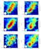 |
Fig. A.1 Maps of the molecules belonging to the c-C3H2 family observed in L1544. The black dashed lines represent the 90%, 50%, and 30% of the H2 column density peak value derived from Herschel maps (Spezzano et al. 2016b), 2.8 × 1022 cm-2. The solid lines represent contours of the molecular integrated emission starting with 3σ with steps of 3σ (the rms of each map is reported in Table 1). The dust peak (Ward-Thompson et al. 1999) is indicated by the black triangle. The white circles represent the HPBW of the 30 m telescope. |
differentiation across L1544. The spectroscopic parameters of the observed lines are summarised in Table 1. In this section we discuss the individual characteristics of the molecules that we have observed.
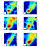 |
Fig. A.1 continued. |
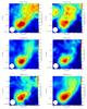 |
Fig. A.1 continued. |
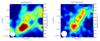 |
Fig. A.1 continued. |
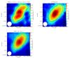 |
Fig. A.2 Maps of the molecules belonging to the dust peak family. |
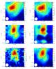 |
Fig. A.3 Maps of the molecules belonging to the methanol peak family. |
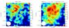 |
Fig. A.3 continued. |
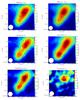 |
Fig. A.4 Maps of the molecules belonging to the HNCO peak family. |
Appendix A.1: The c-C3H2 family
c-C3H2: c-C3H2, cyclopropenylidene, is a three-membered carbon ring. Due to the presence of two unpaired electrons, it has a large dipole moment, 3.27 D (Lovas et al. 1992), and consequently a very bright spectrum in the radio- and mm-band. Cyclopropenylidene was observed in the interstellar medium (ISM) before its detection was confirmed by laboratory work (Thaddeus et al. 1981, 1985a). Since then, it has been detected in a wide variety of sources (Madden et al. 1989; Nakajima et al. 2011). c-C3H2 is an asymmetric top, therefore the labelling of its energy levels is JKa,Kc, with J being the rotational quantum number and Ka and Kc the angular quantum numbers of the prolate and oblate symmetric top limits, respectively. We have mapped two lines of the normal species, c-C3H2 (JKa,Kc = 32,2 − 31,3 and JKa,Kc = 20,2 − 11,1 ), and one of the 13C-species with the 13C off of the principal axis of the molecule (JKa,Kc = 21,2–10,1).
H2CCC (l-C3H2): H2CCC, propadienylidene, is the linear and less stable isomer of cyclopropenylidene. Propadienylidene is usually not as widespread as its cyclic isomer. After its first detection in the laboratory (Vrtilek et al. 1990), it was detected in TMC-1, in IRC+10216 (Cernicharo et al. 1991; Kawaguchi et al. 1991), and in few other Galactic sources (Liszt et al. 2012). The cyclic-to-linear (hereafter c/l) ratio of C3H2 tends to increase with increasing AV. Significant variations of this ratio are found in dense cores, ranging from 25 in TMC-1(CP) to 67 in TMC-1C (Spezzano et al. 2016a; Sipilä et al. 2016). We have mapped two rotational transitions of H2CCC, namely the JKa,Kc = 50,4–40,4 at 103.9 GHz, and the JKa,Kc = 41,3–31,2 at 83.9 GHz.
C3H: The linear C3H is a radical with a 2Π electronic ground state. Given the presence of both the electronic orbital and the spin angular momentum, two ladders of rotational levels are present (Ω = 1/2 and 3/2), which are described by Hund’s “a” case. Here we have mapped two hyperfine transitions (ΔF = 1) in the J = 9/2–7/2 transition of the 2Π1 / 2 ground state. C3H has been observed in IRC+10216 and TMC-1 (Thaddeus et al. 1985b) before its first laboratory detection (Gottlieb et al. 1985, 1986), and it has subsequently been observed towards several sources, among those aretranslucent molecular clouds (Turner et al. 2000), a protoplanetary nebula (Pardo & Cernicharo 2007), and Sgr B2 (McGuire et al. 2013).
C4H: C4H is a radical with  electronic ground state, and its rotational spectrum is split into fine and hyperfine structures given the presence of electron and proton spin. We have mapped the F = 12–11 and 13–12 hyperfine lines (not resolved) of the N = 12–11 transition. C4H was observed in the late 70s towards IRC+10216 (Guelin et al. 1978) before a laboratory spectrum was available, and its astronomical detection was later confirmed by the observations of lower rotational transitions in TMC-1 (Guelin et al. 1982). Its first laboratory spectrum was detected in a Zeeman-modulated spectrometer by Gottlieb and coworkers (Gottlieb et al. 1983). It has now been detected in a wide range of sources, from photodissociation regions (Cuadrado et al. 2015) to dark clouds (Kaifu et al. 2004).
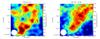 |
Fig. A.5 Maps of the molecules belonging to the category “Others”. |
H2CCO: The microwave spectrum of ketene, H2CCO, was observed for the first time in the laboratory in the 1950s (Johnson & Strandberg 1952). In space, it has been detected in both dark and translucent clouds (Ohishi et al. 1991; Turner et al. 1999; Turner 1977). We have mapped the JKa,Kc = 51,5–41,4 and JKa,Kc = 51,4–41,3 transitions of H2CCO.
HCCNC: HCCNC, ethynyl isocyanide, is an isomer of HC3N, cyanoacetylene. It was first observed in the laboratory in 1992 by means of Fourier transform microwave spectroscopy (Guarnieri et al. 1992) and observed in space by Kawaguchi et al. (1992), towards TMC-1. We have mapped one transition of HCCNC, the J = 9–8.
H2CS: The millimetre- and submillimetre-wave spectrum of thioformaldehyde was studied in the early 70s (Johnson et al. 1971). It was observed in hot cores (Sinclair et al. 1973), dark clouds (Irvine et al. 1989), and circumstellar envelopes (Agúndez et al. 2008). Here we present the map of the JKa,Kc = 30,3–20,2 transition.
HCS+: HCS+ was observed in the ISM (Thaddeus et al. 1981) prior to its laboratory detection (Gudeman et al. 1981). It is a small cation with 1Σ+ electronic ground state. We have mapped the J = 2–1 rotational transition.
C34S: CS is a very abundant and widely distributed interstellar molecule. Towards starless cores, it presents the same abundance drop towards the centre as CO (Tafalla et al. 2004). Here we present the map of the J = 2–1 transition of 34SO towards L1544.
CCS: Thioethenylidene, CCS, is a radical with electronic ground state  . Its rotational energy levels are described by the quantum numbers J and N, referring respectively to the total angular momentum and to the angular momentum of the molecular frame, following Hund’s “b” case. CCS was observed for the first time in the laboratory and in space in 1987 (Saito et al. 1987), and since then it has been observed in different kind of media, from dense to diffuse clouds. Furthermore, it was one of the first molecules mapped in L1544 (Ohashi et al. 1999). We have mapped the N,J = 8, 7–7, 6; 7, 6–6, 5; 7, 7–6, 6; and 8, 9–7, 8 transitions.
CH3CN: Methyl cyanide was among the first molecules detected in the ISM (Solomon et al. 1971). Given its high abundance, also its rarer isotopologues with 13C, D and 15N have been observed (Cummins et al. 1983; Guelin et al. 1982; Nummelin et al. 1998). CH3CN is prolate symmetric top rotor, hence its rotational levels are labelled JK. We have mapped the JK = 60–50 rotational transition at 110 GHz.
HCC13CN: Cyanoacetylene is a linear molecule belonging to the family of cyanopolyyne (HCnN with n = 1, 3, 5, ...). Given the presence of low lying vibrational levels (bending modes), the vibrationally excited states of the normal isotopologue have also been detected in the ISM (Wyrowski et al. 2003). Here we present the map of the J = 10–9 rotational transition.
Appendix A.2: The dust peak family
H13CN: HCN has been observed in a great variety of astrophysical environments, and several vibrationally excited states have been observed towards IRC+10216 (Cernicharo et al. 2011). Being a linear molecule, it has a relatively simple spectroscopy and its rotational levels are described by the quantum numbers J and F, because of the hyperfine structure due to the presence of the nitrogen atom. We mapped the F = 2–1 hyperfine component of the J = 1–0 rotational transition.
13CN: Cyanogen is a radical with 2Σ+ electronic ground state. Like some other astronomically abundant ions and radicals, also CN has been observed in the ISM (Penzias et al. 1974) prior to its laboratory detection (Dixon & Woods 1977). The spectrum of the 13CN isotopologue is characterised by a fine structure given by the interaction of the electron spin and the nuclear rotation, and a hyperfine structure rising from the presence of the 13C and the nitrogen atom. We have mapped the N = 1–0, F1 = 2–1, F2 = 2–1, F = 3–2 transition of 13CN in L1544.
N2H+: N2H+ is a molecular ion with 1Σ+ electronic ground state. Its spectrum is complicated by the presence of two nitrogen atoms, and its J = 1–0 transition is split in to seven hyperfine components (Caselli et al. 1995). N2H+ has been widely observed in dense cores, and it has a crucial importance in astrochemistry because it is a proxy of N2, not observable because it lacks dipole moment. Furthermore N2H+ does not suffer significant depletion like CO and, like other N-bearing molecules, is a very good tracer of the cold inner parts of starless cores. Here we mapped the J = 1–0 F1 = 0–1 F = 1–2 hyperfine transition of N2H+. Maps of N2H+ and N2D+ have already been reported in Caselli et al. (2002).
Appendix A.3: The methanol peak family
CH3OH: Methanol is the smallest complex molecule in the ISM, and it has been extensively observed in dark clouds (e.g. Pratap et al. 1997) and star forming regions (e.g. Bachiller 1996). Given the presence of the CH3 internal rotor, the resulting rotational-torsional spectrum is fairly complicated. Its torsional potential possesses three equivalent minima which lead to rotational transitions of symmetry A or E (doubly degenerated). Levels of different symmetry do not interact, hence the rotational transitions are labelled also with the symmetry state. In our case, we mapped the JKa,Kc = 21,2–11,1 transition of the (E2) state and the JKa,Kc = 00,0–11,1 transition of the (E1-E2) state. This map has already been reported in Bizzocchi et al. (2014) and Spezzano et al. (2016b).
SO and 34SO: SO is a radical with ground state. Its rotational energy levels are described by the quantum numbers J and N, like for CCS. SO and 34SO have been extensively observed in star forming regions and also in extragalactic sources (Martín et al. 2003). Here we present the map of the N,J = 2, 2–1, 1 and 3, 2–2, 1 lines of the main species, and the N,J = 2, 3–1, 2 line for the 34SO isotopologue.
SO2: Sulphur dioxide is quite abundant in the ISM, in particular its lines together with the lines of methanol dominate the spectrum at submillimetre wavelenghts in star-forming regions (Sutton et al. 1991). SO2 is a prolate asymmetric rotor, so its rotational energy levels are described by the quantum numbers JKa,Kc. We have mapped the JKa,Kc = 31,3–20,2 rotational transition.
OCS: OCS is a linear molecule with a simple spectrum with transitions every ~12 GHz. It was detected for the first time in the ISM in the early 70s (Jefferts et al. 1971) and it has been so far observed in a wide variety of media. Furthermore, it is the only S-bearing molecule detected in interstellar ices (Boogert et al. 2015). Here we present the map the of J = 7–6 transition at 85.139 GHz.
HCO: The formyl radical, HCO has been observed towards both diffuse and dense clouds (Liszt et al. 2014; Agúndez et al. 2015). The interaction of the electron spin with the rotation of the molecule splits each rotational level into a doublet. An additional split is caused by the magnetic interaction of the electron spin with the hydrogen nuclear spin. The NKa,Kc = 10,1–00,0 rotational transition has six hyperfine components, here we present the map of one hyperfine component, namely the J = 3/2–1/2 F = 2–1.
Appendix A.4: The HNCO peak family
CH3CCH, CH2DCCH and CH3CCD: Propyne (methyl acetylene) is a stable hydrocarbon, whose spectrum has long been studied in the laboratory (Müller et al. 2000) and in space (Snyder & Buhl 1973; Irvine et al. 1981). While the normal species is a symmetric rotor, and its rotational levels can be labelled with the J and K quantum numbers, the substitution of one hydrogen with deuterium in the methyl group (CH3), breaks the symmetry and three quantum numbers are necessary to describe the spectrum of CH2DCCH. We have mapped the JK = 50-40 line of CH3CCH and the JK = 61–51 line of CH3CCD, and the JKa,Kc = 60,6–50,5 line of CH2DCCH.
HNCO: Isocyanic acid (HNCO) has been vastly studied both in the laboratory and in the ISM. Also its isomer, HCNO, has been observed in space (Marcelino et al. 2009), and very recently its deuterated isotopologue (Coutens et al. 2016). Gas-phase models fail to reproduce the observed abundances of HNCO, and the formation on icy mantels of dust grains has been proposed and tested experimentally (Jiménez-Escobar et al. 2014). HNCO has been linked to the formation of formamide (NH2CHO), a prebiotic interstellar molecule (López-Sepulcre et al. 2015). We have mapped the JKa,Kc = 40,4–30,3 and JKa,Kc = 50,5–40,4 lines of HNCO.
Appendix A.5: Others
13CS: We have mapped the J = 2–1 transition of 13CS. While the less abundant isotopologue C34S belongs to the c-C3H2 family, the 13C isotopologue is more abundant and shows a diffuse distribution, it hence does not belong to any of the categories above.
HC18O+: HCO+, protonated carbon monoxide, was observed in 1970 towards several high mass start forming regions by (Buhl & Snyder 1970). The carrier of this line with “unknown extraterrestrial origin” was proposed to be HCO+ by Klemperer (1970). The detection was not definitive until the first laboratory
detection of HCO+ (Woods et al. 1975). The maps of H13CO+ (J = 1–0) and DCO+ (J = 2–1 and 3–2) have already been presented in Caselli et al. (2002). Here we present the map of the J = 1–0 of HC18O+.
Appendix B: Principal component analysis
In order to decide which was the most rigorous way to carry the principal component analysis on our dataset, we performed it on the raw data, on the standardised data as in Ungerechts et al. (1997), and on the reparametrised data as in Gratier et al. (2017), and compared the different results.
In Gratier et al. (2017) the reparametrisation is done using the following formula:  (B.1)where the a parameter is 8 × 0.08 K, with 0.08 K being the median of the noise among all the maps in his dataset. The parameter a was optimised so that it would maximise the correlation (quantified with the Spearman’s correlation coefficient) of the PC maps with three physical maps of the region, namely the H2 column density, the volume density and the UV illumination. In our case we could not optimise the a parameter as done in Gratier et al. (2017) because the value of the Spearman’s
correlation coefficient of the physical maps of L1544 with the PC maps does not change substantially when varying the parameter a. The results provided here on the reparametrised data use a = 15 × 0.016 K, where 0.016 K is the median of the noise of our maps.
The maps before and after the reparametrisation and standardisation are shown in Figs. B.1–B.3. The results of the analysis on the raw data and on the reparametrised data are reported in Figs. B.4–B.9. When comparing the PC maps obtained on the raw data and on the data that have been reparametrised or standardised, we can see that there is no substantial difference in their shapes. In contrast with what has been done in previous works, we have not included in our dataset the maps of very bright lines (12CO for example), and hence the dynamic range in our dataset is not as large. As a consequence, calculating the eigenvectors and eigenvalues on the covariance or correlation matrix does not produce results which are very different from each other. Still, there are some differences and they should be taken into account in order to perform a rigorous analysis of the results. In both the case of the raw data and with the reparametrisation from Gratier et al. (2017), the first PC map accounts for ~80% of the total correlation and peaks towards the HNCO peak, while in the standardised data the first PC map accounts for ~65% and it peaks towards the c-C3H2 and HNCO peak. This difference can be explained by the fact that the brightest lines in our sample are those from HNCO and CH3CCH, they peak towards the HNCO peak and they dominate the results in the case of performing the PCA on the raw data and on the reparametrised data. This is clear if we look at the emission maps before and after the reparametrisation and the standardisation in Figs. B.1–B.3. While the reparametrised data already show a decrease in the intensity of the emission of the brightest lines (i.e. CH3OH and CH3CCH), it is only when the data are standardised that the differences between bright and weak lines are equalised. For these reasons we decided to focus our discussion on the results of the analysis performed on the standardised data.
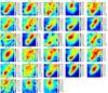 |
Fig. B.1 Raw dataset. The colour scale shows the integrated emission in K km s-1. |
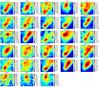 |
Fig. B.2 Dataset after the reparametrisation following the method reported in Gratier et al. (2017). The colour scale shows the integrated emission in K km s-1. |
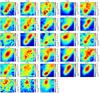 |
Fig. B.3 Dataset after the standardisation following the method reported in Ungerechts et al. (1997). The colour scale shows the integrated emission in K km s-1. |
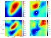 |
Fig. B.4 Maps of the first four principal components obtained by performing the PCA on the raw data. The blue, black, white, and grey diamonds indicate the dust, the HNCO, the c-C3H2, and the methanol peaks respectively. |
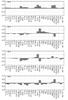 |
Fig. B.5 Contribution of each molecule to the first four PC, obtained by performing the PCA on the raw data. |
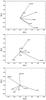 |
Fig. B.6 Correlation wheels where each molecule has as coordinates their correlation coefficients to each PC, obtained by performing the PCA on the raw data. |
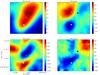 |
Fig. B.7 Maps of the first four principal components obtained by performing the PCA on data reparametrised as in Gratier et al. (2017). The change of sign of PC3 and PC5 with respect to the maps in Fig. B.4 depends on the value of the parameter a, which in our case is arbitrarily chosen (see text). The blue, black, white, and grey diamonds indicate the dust, the HNCO, the c-C3H2, and the methanol peaks respectively. |
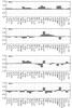 |
Fig. B.8 Contribution of each molecule to the first four PC, obtained by performing the PCA on data reparametrised as in Gratier et al. (2017). |
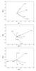 |
Fig. B.9 Correlation wheels where each molecule has as coordinates their correlation coefficients to each PC, obtained by performing the PCA on data reparametrised as in Gratier et al. (2017). |
All Tables
Spectroscopic parameters of the observed lines, divided depending on the position of their emission peaks.
Eingenvalues and eigenvectors derived from principal component analysis on the standardised data.
Spearman’s rank correlation coefficients computed between the physical maps and the first three principal components.
All Figures
|
Fig. 1 Sample of maps belonging to the different families observed towards L1544. The full dataset is shown in Appendix A. The black dashed lines represent the 90%, 50%, and 30% of the H2 column density peak value derived from Herschel maps (Spezzano et al. 2016b), 2.8 × 1022 cm-2. The solid lines represent contours of the molecular integrated emission starting with 3σ with steps of 3σ (the rms of each map is reported in Table 1). The dust peak (Ward-Thompson et al. 1999) is indicated by the black triangle. The white circles represent the HPBW of the 30 m telescope. |
| In the text | |
|
Fig. 2 Maps of the first four principal components obtained by performing the PCA on the standardised data. The maps are constructed by summing for each pixel the contribution of each molecular transition scaled by the values reported in Table 2, i.e. they represent each pixel projected in the space of the principal components. The percentages represent the amount of correlation that can be reproduced by the single principal component. The blue, black, white, and grey diamonds indicate the dust, the HNCO, the c-C3H2, and the methanol peaks respectively. |
| In the text | |
|
Fig. 3 Contribution of each molecular transition to the first four PC, obtained by performing the PCA on the standardised data. |
| In the text | |
|
Fig. 4 Correlation wheels where each molecule has as coordinates their correlation coefficients to each PC, obtained by performing the PCA on the standardised data. |
| In the text | |
|
Fig. 5 Maps of the H2 column density and the dust temperature in L1544. |
| In the text | |
|
Fig. A.1 Maps of the molecules belonging to the c-C3H2 family observed in L1544. The black dashed lines represent the 90%, 50%, and 30% of the H2 column density peak value derived from Herschel maps (Spezzano et al. 2016b), 2.8 × 1022 cm-2. The solid lines represent contours of the molecular integrated emission starting with 3σ with steps of 3σ (the rms of each map is reported in Table 1). The dust peak (Ward-Thompson et al. 1999) is indicated by the black triangle. The white circles represent the HPBW of the 30 m telescope. |
| In the text | |
|
Fig. A.1 continued. |
| In the text | |
|
Fig. A.1 continued. |
| In the text | |
|
Fig. A.1 continued. |
| In the text | |
|
Fig. A.2 Maps of the molecules belonging to the dust peak family. |
| In the text | |
|
Fig. A.3 Maps of the molecules belonging to the methanol peak family. |
| In the text | |
|
Fig. A.3 continued. |
| In the text | |
|
Fig. A.4 Maps of the molecules belonging to the HNCO peak family. |
| In the text | |
|
Fig. A.5 Maps of the molecules belonging to the category “Others”. |
| In the text | |
|
Fig. B.1 Raw dataset. The colour scale shows the integrated emission in K km s-1. |
| In the text | |
|
Fig. B.2 Dataset after the reparametrisation following the method reported in Gratier et al. (2017). The colour scale shows the integrated emission in K km s-1. |
| In the text | |
|
Fig. B.3 Dataset after the standardisation following the method reported in Ungerechts et al. (1997). The colour scale shows the integrated emission in K km s-1. |
| In the text | |
|
Fig. B.4 Maps of the first four principal components obtained by performing the PCA on the raw data. The blue, black, white, and grey diamonds indicate the dust, the HNCO, the c-C3H2, and the methanol peaks respectively. |
| In the text | |
|
Fig. B.5 Contribution of each molecule to the first four PC, obtained by performing the PCA on the raw data. |
| In the text | |
|
Fig. B.6 Correlation wheels where each molecule has as coordinates their correlation coefficients to each PC, obtained by performing the PCA on the raw data. |
| In the text | |
|
Fig. B.7 Maps of the first four principal components obtained by performing the PCA on data reparametrised as in Gratier et al. (2017). The change of sign of PC3 and PC5 with respect to the maps in Fig. B.4 depends on the value of the parameter a, which in our case is arbitrarily chosen (see text). The blue, black, white, and grey diamonds indicate the dust, the HNCO, the c-C3H2, and the methanol peaks respectively. |
| In the text | |
|
Fig. B.8 Contribution of each molecule to the first four PC, obtained by performing the PCA on data reparametrised as in Gratier et al. (2017). |
| In the text | |
|
Fig. B.9 Correlation wheels where each molecule has as coordinates their correlation coefficients to each PC, obtained by performing the PCA on data reparametrised as in Gratier et al. (2017). |
| In the text | |
Current usage metrics show cumulative count of Article Views (full-text article views including HTML views, PDF and ePub downloads, according to the available data) and Abstracts Views on Vision4Press platform.
Data correspond to usage on the plateform after 2015. The current usage metrics is available 48-96 hours after online publication and is updated daily on week days.
Initial download of the metrics may take a while.