| Issue |
A&A
Volume 605, September 2017
|
|
|---|---|---|
| Article Number | A106 | |
| Number of page(s) | 10 | |
| Section | Stellar structure and evolution | |
| DOI | https://doi.org/10.1051/0004-6361/201731040 | |
| Published online | 18 September 2017 | |
Effects of axions on Population III stars
1 Geneva Observatory, University of Geneva, Maillettes 51, 1290 Sauverny, Switzerland
This email address is being protected from spambots. You need JavaScript enabled to view it.
2 Centre de Sciences Nucléaires et de Sciences de la Matière (CSNSM), CNRS/IN2P3, Univ. Paris-Sud, Université Paris-Saclay, Bâtiment 104, 91405 Orsay Campus, France
3 William I. Fine Theoretical Physics Institute, School of Physics and Astronomy, University of Minnesota, Minneapolis, MN 55455, USA
4 Institut d’Astrophysique de Paris, UMR-7095 du CNRS, Université Pierre et Marie Curie; Sorbonne Universités, Institut Lagrange de Paris, 98bis bd Arago, 75014 Paris, France
Received: 25 April 2017
Accepted: 3 July 2017
Abstract
Aims. Following the renewed interest in axions as a dark matter component, we revisit the effects of energy loss by axion emission on the evolution of the first generation of stars. These stars with zero metallicity are assumed to be massive, more compact, and hotter than subsequent generations. It is hence important to extend previous studies, which were restricted to solar metallicity stars.
Methods. Our analysis first compares the evolution of solar metallicity 8, 10, and 12 M⊙ stars to previous work. We then calculate the evolution of 8 zero-metallicity stars with and without axion losses and with masses ranging from 20 to 150 M⊙.
Results. For the solar metallicity models, we confirm the disappearance of the blue-loop phase for a value of the axion-photon coupling of gaγ = 10-10 GeV-1. We show that for gaγ = 10-10 GeV-1, the evolution of Population III stars is not much affected by axion losses, except within the range of masses 80–130 M⊙. Such stars show significant differences in both their tracks within the Tc–ρc diagram and their central composition (in particular 20Ne and 24Mg). We discuss the origin of these modifications from the stellar physics point of view, and also their potential observational signatures.
Key words: elementary particles / stars: evolution / stars: Population III / stars: massive
© ESO, 2017
1. Introduction
Two well studied particles that may be components of the dark matter are the lightest supersymmetric particle (Goldberg 1983; Ellis et al. 1984) and the axion (Preskill et al. 1983; Abbott & Sikivie 1983; Dine & Fischler 1983). While the former is intensely debated because of null searches for supersymmetry at the Large Hadron Collider (Bagnaschi et al. 2015), axions remain a viable dark matter candidate. Axions were originally proposed as a possible solution to the strong Charge Parity (CP) problem (Peccei & Quinn 1977a,b; Weinberg 1978; Wilczek 1978). In strong interactions, there is no reason for CP-violating effects to be small, and these interactions would disagree violently with experiments unless the coefficient of the CP-violating term, called θ, is tuned to be very small (< 10-10). However, the spontaneous breaking of a global U(1) (Peccei-Quinn (PQ) symmetry) allows for the possibility of a dynamical cancellation of the CP-violating phase in QCD. If the scale associated with the symmetry breaking, fa, is large, interactions between the axion and matter become very weak, rendering the axion nearly invisible (Kim 1979; Shifman et al. 1980; Zhitnitskii 1980; Dine et al. 1981). Because the PQ symmetry is also explicitly broken (the CP-violating θ term is not PQ invariant), the axion picks up a low mass similar to a pion picking up a mass when chiral symmetry is broken. Roughly, ma ~ mπfπ/fa where fπ ≈ 92 MeV, is the pion decay constant, so that  (1)As dark matter candidates, axions act as cold dark matter despite their low mass (if fa ≫ fπ) because the cosmological energy density in axions consists of their coherent scalar field oscillations. The energy density stored in the oscillations exceeds the critical density (Preskill et al. 1983; Abbott & Sikivie 1983; Dine & Fischler 1983) unless fa ≲ 1012 GeV or ma ≳ 6 × 10⁻⁶ eV.
Although model dependent, the axion has couplings to photons and matter fermions. As a result, they may also be emitted by stars and supernovae (Raffelt 1990). In supernovae (SNe), axions are produced via nucleon-nucleon bremsstrahlung with a coupling gAN ∝ mN/fa. SN 1987A enables us to place an upper limit (Ellis & Olive 1987; Mayle et al. 1988, 1989; Raffelt & Seckel 1988, 1991; Burrows et al. 1990; Keil et al. 1997) on the axion mass of 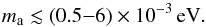 (2)Axion emission from red giants implies (Dearborn et al. 1986; Raffelt & Weiss 1995) ma ≲ 0.02 eV (although this limit depends on the model-dependent axion-electron coupling). From Eq. (1), the limit in Eq. (2) translates into a limit fa ≳ (1 − 12) × 109, implying that only a narrow window exists for axion masses.
In most models, the axion will also couple electromagnetically to photons through the interaction term ℒ = − gaγφaE·B, where φa is the axion field (Raffelt 1990). While not competitive in terms of axion mass limits, the axion-photon coupling, gaγ, can be constrained through several different stellar processes. While axion emission occurs throughout the lifetime of low-mass stars, emission at high temperatures can greatly reduce the lifetime of the helium-burning phase, resulting in an upper limit of g10 ≡ gaγ/ (10-10 GeV-1) < 0.66 (Raffelt & Dearborn 1987; Ayala et al. 2014). A similar limit of g10< 0.8 was derived from the evolution of more massive stars (in the range of 8−12 M⊙) as energy losses in the helium-burning core would overly shorten the blue-loop phase of stellar evolution in these stars (Friedland et al. 2013). For recent reviews, see Kawasaki & Nakayama (2013) and Marsh (2016).
Here we consider the effect of axion emission in more massive but metal-free stars associated with Population III (Pop. III). In such stars we can expect enhanced axions losses compared to solar metallicity stars for at least two reasons. First, we expect higher initial masses for Pop. III stars. The lack of heavy elements prevents dust from forming, and dust is a key agent at solar metallicity to fragment proto-stellar clouds into small pieces of low mass. This is the reason why very few low-mass long-lived stars are believed to be formed in metal-free environments. Only massive or even very massive stars are expected to form (see for instance the review of Bromm 2013). The second reason is that the absence of heavy elements implies that stars of a given initial mass are more compact and thus reach higher central temperatures (see the discussion in Ekström et al. 2008a, for instance).
After describing the process of energy loss by axions in Sect. 2, we use the Geneva code of stellar evolution to confirm in Sect. 3 that axion emission from solar metallicity stars might be constrained by the disappearance of the blue-loop phase. Our goal, however, is to study the axion energy losses for massive Pop. III stars, which is described extensively in Sect. 4. Our conclusions are given in Sect. 5.
2. Energy loss by axions
For a given coupling of axions to photons, Primakoff emission (Primakoff 1951) of axions from photon-nucleus scattering will occur, mediated by the virtual photons from the electrostatic potential of the nucleus (Fig. 1). The screening of this potential by the freely moving electric charges (Debye-Hückel effect) needs to be taken into account, however (Raffelt 1986). The volume emissivity for this process as a function of temperature (for temperatures much greater than the plasma frequency) was computed in Raffelt (1986, 1990).
Dividing this emissivity by the mass density, ρ, we obtain an energy-loss rate per unit mass, 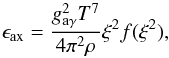 (3)where the function f is defined in Eq. (4.79) of Raffelt (1990) and ξ is given by
  (4)with ħ the reduced Planck constant, c the speed of light, and kB the Boltzmann constant (see the appendix for an explanation of the units). The Debye-Hückel screening wavenumber, kS, is given by Raffelt (2008) as
 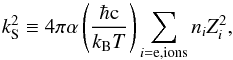 (5)where α is the fine-structure constant, Zi is the atomic number, and ni is the ion or electron number density, given by
 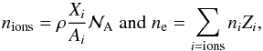 (6)(because of charge neutrality), with
  the Avogadro number. The energy-loss rate (Eq. (3)) can be rewritten as
  (7)where T8 ≡ T/ (108 K) and ρ3 ≡ ρ/ (103 g / cm3). We note that the numerical constant differs from the constant in Eq. (3) of Friedland et al. (2013) by one order of magnitude (see the appendix for more details).
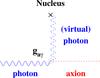 |
Fig. 1 Primakoff effect: a real photon from the thermal bath is converted into an axion by the electric field of a nucleus. |
We correct Eq. (3) by the damping factor introduced by Aoyama & Suzuki (2015), namely, exp( − ħω0/kBT), where ω0 is the plasma frequency in MeV: ![Mathematical equation: \begin{equation} \hbar\omega_0=\left[4\pi\alpha\left(\frac{\hbar\mathrm{c}}{m_{\rm e} c^2}\right)n_{\rm e}\right]^\frac{1}{2}\hbar\mathrm{c}. \label{q:damp} \end{equation}](/articles/aa/full_html/2017/09/aa31040-17/aa31040-17-eq47.png) (8)However, the damping factor always remains of the order of unity in our models.
(8)However, the damping factor always remains of the order of unity in our models.
During the main sequence (MS), most of the energy in massive stars is transported by radiation and convection so that the axions have little effect. Axion cooling is believed to have a significant effect during the core helium-burning phase, when the central temperature and density are about 108 K and 103 g cm-3 (see e.g. Friedland et al. 2013). In the next stages (core carbon burning, oxygen, etc.), the cooling by axions would be more pronounced because of the higher temperature and density. At these late stages, however, the axion cooling competes with neutrino losses. Whether axion losses in Pop. III stars are significant or not compared to other sinks of energy, like neutrino losses, is a point investigated in this paper.
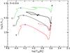 |
Fig. 2 Hertzsprung-Russell diagram for the six models computed at solar metallicity. Dashed lines show models without axion losses. Solid lines show models with axion losses. Circles (without axion losses) and squares (with axion losses) show the location of the models at the end of core He-burning. Blue crosses show the location of the tracks at core helium-burning ignition (ϵ(3α) > 0). |
3. Massive stars with solar metallicity
It was shown that at solar metallicity the energy losses by axions from the helium-burning core can eliminate the blue-loop phase (Friedland et al. 2013). Limits on the axion photon coupling were derived from studies of 8 − 12 M⊙ models. To check whether we find similar results, we have computed models at similar mass and metallicity.
3.1. Physical ingredients
We computed six models of 8, 10, and 12 M⊙ at solar metallicity, with and without energy losses by axions using the Geneva code. Similar input parameters as those used in Ekström et al. (2012) were considered for these computations. The initial abundance of H, He, and metals in mass fractions are X = 0.72, Y = 0.266, and Z = 0.014, respectively. The mixture of heavy elements was determined according to Asplund et al. (2005) except for Ne, whose abundance was taken from Cunha et al. (2006). The isotopic ratios are from Lodders (2003). The core-overshoot parameter dover/Hp = 0.1, where Hp is the pressure scale height determined at the Schwarzschild convective core boundary. It extends the radius of the convective core by an amount of 0.1 Hp. The outer layers, if convective, were treated using the mixing-length theory. The mixing-length parameter αMLT was set to 1.6. This value allow to reproduce the solar radius at the age of the Sun as well as the positions of the red giants and supergiants in the HR diagram (Ekström et al. 2012).
To compute the energy-loss rate per unit mass due to axions, we took g10 = gaγ/ (10-10 GeV-1) = 1 in all our models. The simulations were stopped at the end of the core helium-burning phase. The models are labelled “10g1” for instance, where “10” refers to the initial mass in solar masses and “g1” means g10 = 1.
3.2. Evolution in the Hertzsprung Russell diagram
Figure 2 depicts the evolutionary tracks in the HR diagram. For the 8 M⊙ models (red lines), the blue loop disappears when the energy loss by axions is included (solid red line). To understand this behaviour, we recall that a blue loop appears when the stellar envelope contracts, causing the star to leave the red supergiant branch and to evolve blueward in the HR diagram. During the core He-burning phase, the envelope contracts because the core expands. This is due to the mirror effect. The expansion of the core comes from the fact that when the abundance of helium decreases in the central regions, the central temperature increases. One effect of the increase in central temperature is the increase in nuclear energy generation by reactions such as 12C(α, γ)16O (we note here that the rate of this reaction is still highly uncertain). The excess of nuclear energy is used to expand the core. The appearance or disappearance of the blue loops is very sensitive to many inputs of the stellar models, and small changes can have important effects, such as changes in mesh resolution, the way to account for convection, and the mixing in the radiative zones (see e.g. Kippenhahn & Weigert 1990; Maeder & Meynet 2001; Walmswell et al. 2015).
When energy losses by axions are included, the energy produced by the nuclear reactions in the core is more efficiently removed from the helium-burning core (the energy removed by axions is ≲ 3 × 10⁴ erg g-1 s-1 for the models of this section). This limits the expansion of the helium core, which in turn limits the contraction of the envelope. This finally tends to reduce or even prevent the formation of a blue loop. This change in behaviour is restricted to the 8 M⊙ star in the three models with different initial masses considered here.
3.3. Duration of burning phases
Interestingly, for our 8 M⊙ model, the duration of the helium-burning phase is reduced by ~ 13% when axions are considered. For the 10 and 12M⊙ models, the reduction is ~ 8% and ~ 11%, respectively. Thus we see that the largest effects on the lifetimes are found for the 8 M⊙ case. This does appear somewhat consistent with the fact that the blue loop is affected in this model. The lifetimes are shorter when axions are considered because they add a new channel that is very efficient in removing energy from the core.
Friedland et al. (2013) found a decrease in duration of the helium burning by ~ 23% (cf. their Fig. 3 and discussion) for a 9.5 M⊙ with g10 = 0.8, which exceeds the lifetime decreases that we have obtained here. This might appear surprising in view of their value for g10 that is lower than the value adopted here. Instead, we would have expected that the lifetime decreases reported by Friedland and coauthors would be smaller than those obtained here with a g10 = 1. In all likelihood, our stellar models differ by some other physical ingredients, such as the overshoot parameter. These differences are difficult to trace back, however, because of the lack of details given in Friedland et al. (2013). More importantly, we find similar qualitative trends. Using a different stellar evolution code, we find as in Friedland et al. (2013) that axions suppress the blue loops for some masses and decrease the core He-burning lifetime.
In contrast to the helium-burning phase, the duration of the MS is very little affected by axions because the relevant temperature for axion cooling to be efficient is not reached in the core of massive MS stars. The duration of this phase is reduced by less than ~ 0.1% for our models. The reason is that the losses by axions are very small during this phase.
 |
Fig. 3 Same as Fig. 2, but for the 16 Pop. III models. The shaded area shows the zone of the diagram where helium burns in the core of the models without axion losses. The thin black line shows the location of the models without axion losses when the carbon starts to burn into the core. The shaded area and the black line are similar for models with axion losses. Circles (without axion losses) and squares (with axion losses) show the location of the models at the end of core C-burning. |
4. Pop. III stars
4.1. Physical ingredients
With the same physical ingredients used for solar metallicity models as in the previous section, we calculated Pop. III models of 20, 25, 32, 40, 60, 85, 120, and 150 M⊙ with and without axion losses. The evolution was stopped at the end of core C-burning. We used the mass-loss recipe of Vink et al. (2001). Ṁ depends on (Z/Z⊙)0.85 so that Ṁ should be 0 for our Pop. III models. However, we used Z = 10-4Z⊙ as a threshold value for the mass-loss rate. This was done previously in Marigo et al. (2003) and Ekström et al. (2008a). We note that our models were computed at Z = 0, but we adopted the mass-loss rates for these models that are given by a metallicity Z = 10-4Z⊙. In some models, the opacity peak produced by the variation in the ionisation level of hydrogen decreases the Eddington luminosity LEdd = 4πcGM/κ below the actual luminosity of the star. As a consequence, the external layers of such models exceed the Eddington luminosity. This unstable phase cannot be solved with our hydrostatic approach. It is accounted for by increasing the mass-loss rate by a factor of 3 whenever the luminosity of any of the layers of the stellar envelope is higher than 5LEdd (Ekström et al. 2012).
4.2. Evolutionary tracks in the HR diagram and lifetimes
The tracks in the HR diagram (Fig. 3) are little affected by axion losses. The main differences between the two families of tracks arise close to the end of the evolution, when axion losses are higher than other sources of energy loss. We see that in general, models with axions remain bluer in the HR diagram than the models without axions. Since axions add a new channel for evacuating the energy from the central regions, it removes energy that otherwise might be used to inflate the envelope and push the track in the HR diagram redward. In the previous section, we saw that axions could suppress a blue loop, thus causing a contraction of the envelope. Here we see that axions may reduce the expansion of the envelope. This difference arises here because we considered the impact of axions at a different stages of the evolution. In the previous section, we discussed the case of a core He-burning star at the red supergiant stage. Here we consider stars after the core He-burning phase that still cross the HR gap. In both cases axions remove energy. In the first case, this decreases the ability of the core to extend and hence the envelope to contract. In the second case, it removes energy released by contraction of the core that otherwise is used to expand the envelope. This is what occurs for initial masses below ~85 M⊙. The 120g1 model loses ~20 M⊙ at the end of the core helium-burning phase. Before mass ejection, log Teff ~ 3.8 (solid green line in Fig. 3). While losing mass, log Teff then decreases until it reaches a value of about 4.1. This model loses more mass than the 120g0 model (120 M⊙ without axion) because it remains in a domain of the HR diagram where the luminosity becomes supra-Eddington for a longer time in some outer layers of the star.
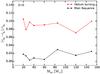 |
Fig. 4 Relative difference of the duration of MS and core helium-burning phases between Pop. III models with (g10 = 1, noted as g1) and without (g10 = 0, noted as g0) axion losses. |
The differences between the tracks in the HR diagram remain very modest. We computed different 85g1 models using different time-steps near the end of the evolution. This leads to slightly different final Teff. The scatter is of the order of the difference in Teff between the 85g0 and 85g1 models shown in Fig. 3. In any case, differences like this cannot be used to constrain the presence of axions. This is true for at least two reasons. (1) Pop. III stars cannot be directly observed and thus they cannot be placed into a HR diagram. With the James Webb Telescope, it will be possible, on the other hand, to detect supernovae from Pop. III stars. From the evolution of their early light curves (during the rise time), it might be possible to obtain some indications on the radius of the core-collapse supernova progenitors (see e.g. Nakar & Sari 2010; Bersten et al. 2012; Dessart et al. 2013; Morozova et al. 2016). However, this radius does not depend only on the presence of the axions. It also depends on convection, mixing in radiative layers, opacities, and mass losses, and thus there is little hope at the moment to use this channel to constrain the physics of axions. (2) Axions may change the lifetimes of stars somewhat. This may indirectly have an impact on the ionizing power of Pop. III stars. Changing the MS lifetime, for instance, will change the duration of the phase when UV photos are emitted by the star. The impact of axions on lifetimes is shown in Fig. 4. We see that axions shorten the MS lifetime by less than 3% and reduce the core helium burning lifetimes by 7 − 10%. As already mentioned above, this simply reflects the fact that the effects of axions are the most marked when temperature increases, i.e. in the more advanced phases of the evolution. Again, here the effects are very modest and of the same order of magnitude as changes that are due to other uncertain physical ingredients of the models. A consequence of a shorter helium lifetime is that the 12C(α, γ)16O reaction has less time to operate during core helium burning so that the 12C/16O ratio at the end of central helium burning is slightly higher (≲ 5%) for models with shorter helium lifetimes, hence with axion losses.
 |
Fig. 5 Coloured lines shows the tracks for the computed Pop. III models in the central temperature vs. central density plane. Dashed lines show models without axion losses, while solid lines show models with axion losses. The ignition of the different burning stages and the end of central helium burning are given for the models without axion losses. The broad dashed Γ < 4 / 3 line indicates the zone of the diagram where electron-positron pair creations lower the adiabatic index below 4/3. The X = 1 and Z = 1 lines show the limit between the perfect gas and the completely degenerate non-relativistic gas for pure hydrogen and pure metal mixtures. Light purple lines delimitate the different regions where a given neutrino source (pair, photoneutrino, bremsstrahlung, and plasma) dominates. The colour map shows the ratio ϵax/ϵν , where ϵν is the sum of the four types of neutrino losses mentioned above, computed according to Itoh et al. (1989, 1996). |
4.3. Central conditions
The coloured lines of Figs. 5 and 6 show the evolution in the (log Tc, log ρc) diagram where Tc and ρc are the central temperature and density, respectively. The colour map shows the ratio ϵax/ϵν between axion and neutrino energy losses. It shows that axions remove more energy than neutrinos from the central regions before the beginning of the core C-burning phase. After C-ignition in the centre, neutrinos dominate. Thus, we can expect that axions will have their most important effects before the core C-burning phase. However, for axions to have a strong impact on the models, it is not sufficient that energy losses by axions are more important than neutrinos, energy losses due to axions must also be important with respect to the energy released either by nuclear reactions or gravitational contraction.
During the core H-burning phase, the energy is mainly transported by radiation and convection. Axion cooling has little effect. The same is also true, although to a smaller extent, during the core He-burning phase. The only phase where strong differences may appear due to axions is during the transition between the end of the core He-burning phase and the beginning of the core C-burning phase. During this phase, energy in the central part is produced by core contraction (see the green line in Fig. 7). After the end of the core He-burning phase, the energy released by the contraction of the core is taken away by axions (between the abscissa 4 and 2.5 in Fig. 7). This is the phase during which axions may induce some significant changes in the models.
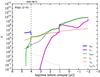 |
Fig. 7 Energy generated by helium burning (ϵHe), carbon burning (ϵC), gravitational energy (ϵgrav), energy of the neutrinos (ϵν), and of the axions (ϵax). Thick lines represent sources of energy, and thin lines represent sinks of energy. The dotted line shows the ratio ϵax / ϵν. The vertical dashed line denotes the end of the core helium-burning phase. |
For most of the models, axions do not have a strong effect. There is an exception, however, in the cases of the 85 and 120 M⊙ models. As can be better seen in Fig. 6, the central density and temperature of the 85g1 (solid black line) and 120g1 (solid green line) models significantly deviates from the models without axions. After the core He-burning phase, the tracks with axions join the tracks of the 40 (cyan tracks) and 32 (yellow tracks) M⊙ models (see Fig. 5), respectively, and follow these tracks until the end of their evolution. In other words, they follow the evolution of stars with lower initial masses.
In these models, larger amounts of energy can be evacuated from the central regions than in models with only neutrinos. This decreases the content of entropy in the core and thus will make the central region more sensitive to degeneracy effects. This explains why the tracks with axions more rapidly approach the line separating the non-degenerate from the degenerate region (see the lines labelled X, Z = 1 in Fig. 6).
Surprisingly, this behaviour disappears above and below the range 85−120 M⊙. Outside this specific mass range, axions no longer have important effects, and the tracks are only slightly changed when axions are considered. To understand why this situation arises, we note the following:
-
As indicated above, axions dominate the process of energyremoval from the central regions just after the core He-burningphase, until neutrinos become dominant. The durations of thisphase, obtained in the different initial mass models computedwith axions, are shown in Fig. 8. We see that thelongest axion-dominated phases occur for the 85 and120 M⊙ models. This is consistent with the fact that axions have the strongest impact in these models. The 20 M⊙ model also has a rather long axion-dominated phase. A careful examination of Fig. 5 indicates that the track is more strongly shifted than the other towards lower densities at a given temperature. This shift disappears after C-ignition in the core, however.
-
The duration of the axion-dominated phase can be estimated to first order as
 , where Mcore, Rcore are the mass and the radius of the core at the end of the core He-burning phase, respectively, and Laxion is the axion luminosity. This equation expresses the fact that during this phase, the energy source is mainly the gravitational energy, i.e.
  . The gravitational energy increases with the mass. The axion luminosity increases rapidly with the temperature, and the temperature also increases with the mass. Therefore both the numerator and the denominator increase with the mass. This prevents an easy prediction of how the ratio will vary as a function of mass. Current numerical models tell us that for most of the initial masses, this ratio keeps a nearly constant value. For a few initial masses, this ratio is higher, however.
4.4. Internal structure of the 85 and 120 M⊙ models
The structure evolution of the of the 85g1 and 120g1 models shows striking differences compared to the 85g0 and 120g0 models. This is illustrated in Fig. 9, which compares the evolution as a function of time of the convective regions (grey areas) in the 85g0 and 85g1 models. We see that the core hydrogen- and helium-burning phases are very similar in both models. Differences appear after the core He-burning phase. In the model without axions, we have two convective burning shells during the whole post-He-burning phase. The outer shell is the convective H-burning shell, and the inner shell is the convective He-burning shell. In the models with axions, before C-ignition, there is only one convective burning shell, the He-burning shell. We also see that during this phase, the convective He-burning shell in the model with axions is more extended than in the model without axions. This is because in models with axion losses, more energy is removed from the He-shell and below. As a consequence, the star contracts more strongly in this region. This tends to make this region warmer, which in turn boosts the He-burning energy generation in the region where helium is still present. As a consequence, this convective region extends farther.
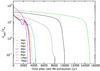 |
Fig. 8 ϵax/ϵν ratio in the core of Pop. III models as a function of the time after the end of central helium burning. |
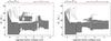 |
Fig. 9 Kippenhahn diagram of the 85g0 (left) and 85g1 (right) models. Grey areas represent the convective zones. The red line at the top shows the total mass. The core hydrogen-, helium-, and carbon-burning phases are indicated at the top of the panels. |
Because of the additional energy removed by axions, the cores of the 85g1 and 120g1 models contract more strongly than the cores of the 85g0 and 120g0 models. This leads to a high central density that makes the cores of the 120g1 and 85g1 models partially degenerate. In this case, the energy released by contraction is in part used to push some electrons to occupy higher energy quantum levels. This energy is not used to increase the thermal energy. This implies that the 85g1 and 120g1 models end their evolution with a lower central temperature than the 85g0 and 120g0 models (see Fig. 6). We recall that on the other hand, the 85g1 and 120g1 models end their evolution with a higher temperature in the He-shell than the 85g0 and 120g0 models (cf. the discussion in this section).
The structure of these models during this stage (in between helium and carbon burning) is nevertheless sensitive to other parameters, like the resolution (number of shells). We again computed the 85g1 model with a different resolution, and the convective pattern from abscissa ~ 4 in Fig. 9 (right panel) is different. This illustrates once again that other parameters can impact the structure of the models during specific phases. It remains, nevertheless, that the effect of the axions is the strongest during that stage (cf. Fig. 8 and discussion). This is to say, during this stage, the axions are most likely to have an impact on the evolution or structure of the star.
In addition, the structure changes mentioned above are present only for a period of time. They appear as a transitory reaction of the model to the increased loss of energy in the central regions. In the end, the models converge towards structures that are again very similar (compare the two structures shown in Fig. 9 at the very end of the evolution). The final masses of the helium and carbon-oxygen cores are little affected by the effect of axions (see Table 1).
Masses of the helium and carbon-oxygen cores at the end of the core C-burning phase.
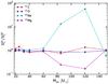 |
Fig. 10 Ratio of central abundances at the end of core C-burning between models with axion losses ( |


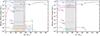 |
Fig. 11 Abundance profiles of the 85g0 (left) and 85g1 (right) models at the end of core carbon burning (central mass fraction of 12C below 10-5). The shaded area shows the convective zones. |
It is interesting to note that although the 85 and 120 M⊙ stars with axions would have very similar masses for the He and CO cores compared to their siblings without axions, they nevertheless show central conditions that are very different. As seen in Fig. 6, they show much higher densities at a given temperature, thus, as already underlined above, the models with axions are much more sensitive to degeneracy effects. Whether this produce some flashes or even an explosion in the presupernova phases remains to be explored.
Recently, Woosley (2017) has investigated the final evolution of 70 − 140M⊙ stars. He found that such stars should experience pulsational pair-instability supernovae (PPISN). PPISN would occur if the final helium core is more massive than 30 M⊙. For helium cores above 62 M⊙, the star is disrupted as a single pulse (pair-instability supernovae). Our 85, 120, and 150 M⊙ models have helium cores of between ~ 37 and 68 M⊙ (see Table 1). They might experience PPISN (or PISN for helium cores above 62 M⊙). However, the axion cooling might prevent our 85 and 120 M⊙ models from entering in the unstable regime (see Figs. 5 and 6). If so, such stars could produce black holes in the mass range where no black hole is usually expected, between 64 and 133 M⊙ (Heger & Woosley 2002). This could induce a potential signature in gravitational waves. Although still far from being able to use stellar models to verify the existence of axions, this possible axion signature has to be kept in mind for the future.
4.5. Impact of the axion cooling on nucleosynthesis
Population III stars lose very little mass through stellar winds (although fast rotation may change this picture, see Ekström et al. 2008a,b). The only way they can contribute to nucleosynthesis would therefore be through supernova ejecta. As discussed above, the two masses for which the impact of axions are strongest are the 85 and 120 M⊙. If these two stars would end their life producing a black hole with very little or no mass ejecta, then their contribution in enriching the interstellar medium would likely be null. However, a successful explosion is also a possible scenario (e.g. Ertl et al. 2016; Sukhbold et al. 2016). The discussion below investigates the possible impact of axions when some material is ejected.
Figure 10 shows central abundance ratios at the end of core C-burning for models with and without axions losses. The most abundant species are shown. The central abundances of 20 − 60M⊙ models are little affected by axion losses. Over the whole range of masses considered, 12C and 16O are little affected. 20Ne and 24Mg are affected in the range 80−140 M⊙. The central 20Ne (24Mg) abundance is ~ 60 times higher (~ 5 times lower) in the 120g1 model than in the 120g0 model. This is due to the higher central temperature in the 85g0 (120g0) compared to the 85g1 (120g1) model (cf. discussion in Sect. 4.3). In the case of the 85g0 and 120g0 models, the central temperature reaches values > 1.4 GK, where the 20Ne(α, γ)24Mg channel becomes stronger than the 16O(α, γ)20Ne channel, so that significantly more 24Mg is synthesized, to the detriment of 20Ne. However, the central abundances are not sufficient to determine the yield of an element. The complete chemical structure should be inspected.
Figure 11 shows the complete chemical structure obtained in the two 85 M⊙ models with and without axions. These structures are also representative of the 120 M⊙ models. For the other models, the axions do not lead to significant differences in the final abundance profiles, and we do not discuss them further. We see in Fig. 11 that the distribution of oxygen is very similar in both models, and we therefore do not expect important effects on the stellar yield of this element. For 12C, we see some differences: the zone where carbon is depleted is smaller for the 85g1 model. This is because the cooling due to axion emission is more efficient before the core carbon-burning phase. This implies that a smaller fraction of the core reaches the conditions needed for carbon burning to occur. The 14N profiles are slightly different, but the mass fraction stays very small, below 10-5 in any case. This difference is not significant.
In the He-burning shell, the abundances of 20Ne and 24Mg are larger in the model with axions. These differences reflect the higher temperatures reached in the He-burning shell in the model with axions (cf. discussion in Sect. 4.3). On the whole, we see that when these layers that are associated with the He-burning shell are ejected, this may boost the yield by a factor 10 with respect to the yield of these two isotopes obtained in the corresponding models without axions. However, this will occur in a relatively short mass range, and the global effect on the yields integrated over an initial mass function where these massive stars are far out-numbered by lower mass stars will therefore remain quite modest.
5. Conclusions
We have explored the impact of axions in massive stars at solar metallicity and in Pop. III stars. In solar metallicity stars, we have confirmed that the axion coupling to photons might be constrained by the disappearance of the blue-loop phase in stars with masses between 8 and 12 M⊙. However, caution is required because blue loops are very sensitive to many other uncertain physical processes (e.g. core convection and its efficiency and boundary mixing), which can also remove the blue loops from a stellar evolutionary track without need for axion cooling. In Pop. III stars, we have shown that the effects of axions on stellar evolution are very modest and are hardly observable, mainly because uncertainties in other parameters of stellar models produce effects at least as strong.
The most spectacular effect of axions explored in the present work is on the physical conditions obtained at the end of the evolution for Pop. III stars with masses between about 80 and 130 M⊙. These stars present cores with some level of degeneracy, and the final fate of these objects is not clear. Sukhbold et al. (2016) have investigated the final fate of 9−120 M⊙ solar metallicity models. Above 30 M⊙, most of the models do not explode and form black holes. The effect of axions might change this picture. This clearly needs further investigation, especially as we approach the era of observations with the James Webb Telescope, which might detect supernovae in the entire observable Universe. Such stars might give rise to a type of explosive event with a clear non-ambiguous signature inherited from the particular structure of their progenitors.
In a broader perspective, this work shows that we are still far from a situation where Pop. III stellar models can be used as a physics laboratory to verify the presence of axions, and even farther from the situation where stars might constrain their properties. This shows the importance of continuing our efforts in stellar physics, making stellar models still more precise and reliable so that real stars can be used as physics laboratories, which will open new windows on questions at the frontier of physics, in the domain of temperatures and densities that are not reachable in a laboratory.
Acknowledgments
We would like to thank Jordi Isern for useful discussions during the early stage of this project. The work of K.A.O. was supported in part by DOE grant DE-SC0011842 at the University of Minnesota. The work of E.V. has been carried out at the ILP LABEX (under the reference ANR-10-LABX-63) supported by French state funds managed by the ANR within the Investissements d’Avenir programme under reference ANR-11-IDEX-0004-02.
References
- Abbott, L. F., & Sikivie, P. 1983, Phys.Lett. B, 120, 133 [Google Scholar]
- Aoyama, S., & Suzuki, T. K. 2015, Phys. Rev. D, 92, 063016 [NASA ADS] [CrossRef] [Google Scholar]
- Asplund, M., Grevesse, N., & Sauval, A. J. 2005, in Cosmic Abundances as Records of Stellar Evolution and Nucleosynthesis, eds. T. G. Barnes, III, & F. N. Bash, ASP Conf. Ser., 336, 25 [Google Scholar]
- Ayala, A., Domínguez, I., Giannotti, M., Mirizzi, A., & Straniero, O. 2014, Phys. Rev. Lett., 113, 191302 [NASA ADS] [CrossRef] [Google Scholar]
- Bagnaschi, E. A., Buchmueller, O., Cavanaugh, R., et al. 2015, Eur. Phys. J C, 75, 500 [Google Scholar]
- Bersten, M. C., Benvenuto, O. G., Nomoto, K., et al. 2012, ApJ, 757, 31 [NASA ADS] [CrossRef] [Google Scholar]
- Bromm, V. 2013, Rep. Prog. Phys., 76, 112901 [Google Scholar]
- Burrows, A., Ressell, M. T., & Turner, M. S. 1990, Phys. Rev. D, 42, 3297 [NASA ADS] [CrossRef] [Google Scholar]
- Cunha, K., Hubeny, I., & Lanz, T. 2006, ApJ, 647, L143 [NASA ADS] [CrossRef] [Google Scholar]
- Dearborn, D. S. P., Schramm, D. N., & Steigman, G. 1986, Phys. Rev. Lett., 56, 26 [NASA ADS] [CrossRef] [PubMed] [Google Scholar]
- Dessart, L., Hillier, D. J., Waldman, R., & Livne, E. 2013, MNRAS, 433, 1745 [NASA ADS] [CrossRef] [Google Scholar]
- Dine, M., & Fischler, W. 1983, Phys. Lett. B, 120, 137 [NASA ADS] [CrossRef] [Google Scholar]
- Dine, M., Fischler, W., & Srednicki, M. 1981, Phys. Lett. B, 104, 199 [NASA ADS] [CrossRef] [Google Scholar]
- Ekström, S., Meynet, G., Chiappini, C., Hirschi, R., & Maeder, A. 2008a, A&A, 489, 685 [NASA ADS] [CrossRef] [EDP Sciences] [Google Scholar]
- Ekström, S., Meynet, G., & Maeder, A. 2008b, in Massive Stars as Cosmic Engines, eds. F. Bresolin, P. A. Crowther, & J. Puls, IAU Symp., 250, 209 [Google Scholar]
- Ekström, S., Georgy, C., Eggenberger, P., et al. 2012, A&A, 537, A146 [NASA ADS] [CrossRef] [EDP Sciences] [Google Scholar]
- Ellis, J., & Olive, K. A. 1987, Phys. Lett. B, 193, 525 [NASA ADS] [CrossRef] [Google Scholar]
- Ellis, J., Hagelin, J. S., Nanopoulos, D. V., Olive, K., & Srednicki, M. 1984, Nucl. Phys. B, 238, 453 [Google Scholar]
- Ertl, T., Janka, H.-T., Woosley, S. E., Sukhbold, T., & Ugliano, M. 2016, ApJ, 818, 124 [NASA ADS] [CrossRef] [Google Scholar]
- Friedland, A., Giannotti, M., & Wise, M. 2013, Phys. Rev. Lett., 110, 061101 [NASA ADS] [CrossRef] [Google Scholar]
- Goldberg, H. 1983, Phys. Rev. Lett., 50, 1419 [NASA ADS] [CrossRef] [Google Scholar]
- Heger, A., & Woosley, S. E. 2002, ApJ, 567, 532 [NASA ADS] [CrossRef] [Google Scholar]
- Itoh, N., Adachi, T., Nakagawa, M., Kohyama, Y., & Munakata, H. 1989, ApJ, 339, 354 [NASA ADS] [CrossRef] [Google Scholar]
- Itoh, N., Hayashi, H., Nishikawa, A., & Kohyama, Y. 1996, ApJS, 102, 411 [NASA ADS] [CrossRef] [Google Scholar]
- Kawasaki, M., & Nakayama, K. 2013, Ann. Rev. Nucl. Part. Sci., 63, 69 [NASA ADS] [CrossRef] [Google Scholar]
- Keil, W., Janka, H.-T., Schramm, D. N., et al. 1997, Phys. Rev. D, 56, 2419 [NASA ADS] [CrossRef] [Google Scholar]
- Kim, J. E. 1979, Phys. Rev. Lett., 43, 103 [NASA ADS] [CrossRef] [Google Scholar]
- Kippenhahn, R., & Weigert, A. 1990, Stellar Structure and Evolution (Springer-Verlag) [Google Scholar]
- Lodders, K. 2003, ApJ, 591, 1220 [NASA ADS] [CrossRef] [Google Scholar]
- Maeder, A., & Meynet, G. 2001, A&A, 373, 555 [NASA ADS] [CrossRef] [EDP Sciences] [Google Scholar]
- Marigo, P., Chiosi, C., & Kudritzki, R.-P. 2003, A&A, 399, 617 [NASA ADS] [CrossRef] [EDP Sciences] [Google Scholar]
- Marsh, D. J. E. 2016, Phys. Rep., 643, 1 [NASA ADS] [CrossRef] [Google Scholar]
- Mayle, R., Wilson, J. R., Ellis, J., et al. 1988, Phys. Lett. B, 203, 188 [NASA ADS] [CrossRef] [Google Scholar]
- Mayle, R., Wilson, J. R., Ellis, J., et al. 1989, Phys. Lett. B, 219, 515 [NASA ADS] [CrossRef] [Google Scholar]
- Morozova, V., Piro, A. L., Renzo, M., & Ott, C. D. 2016, ApJ, 829, 109 [NASA ADS] [CrossRef] [Google Scholar]
- Nakar, E., & Sari, R. 2010, ApJ, 725, 904 [NASA ADS] [CrossRef] [Google Scholar]
- Peccei, R. D., & Quinn, H. R. 1977a, Phys. Rev. D, 16, 1791 [NASA ADS] [CrossRef] [Google Scholar]
- Peccei, R. D., & Quinn, H. R. 1977b, Phys. Rev. Lett., 38, 1440 [NASA ADS] [CrossRef] [Google Scholar]
- Preskill, J., Wise, M. B., & Wilczek, F. 1983, Phys. Lett. B, 120, 127 [NASA ADS] [CrossRef] [Google Scholar]
- Primakoff, H. 1951, Phys. Rev., 81, 899 [NASA ADS] [CrossRef] [Google Scholar]
- Raffelt, G. G. 1986, Phys. Rev. D, 33, 897 [NASA ADS] [CrossRef] [Google Scholar]
- Raffelt, G. G. 1990, Phys. Rep., 198, 1 [NASA ADS] [CrossRef] [Google Scholar]
- Raffelt, G. G. 2008, in Axions, Lecture Notes in Physics (Berlin: Springer Verlag), eds. M. Kuster, G. Raffelt, & B. Beltrán, 51, 741 [Google Scholar]
- Raffelt, G. G., & Dearborn, D. S. P. 1987, Phys. Rev. D, 36, 2211 [NASA ADS] [CrossRef] [Google Scholar]
- Raffelt, G., & Seckel, D. 1988, Phys. Rev. Lett., 60, 1793 [NASA ADS] [CrossRef] [Google Scholar]
- Raffelt, G., & Seckel, D. 1991, Phys. Rev. Lett., 67, 2605 [NASA ADS] [CrossRef] [Google Scholar]
- Raffelt, G., & Weiss, A. 1995, Phys. Rev. D, 51, 1495 [NASA ADS] [CrossRef] [Google Scholar]
- Shifman, M. A., Vainshtein, A. I., & Zakharov, V. I. 1980, Nucl. Phys. B, 166, 493 [NASA ADS] [CrossRef] [MathSciNet] [Google Scholar]
- Sukhbold, T., Ertl, T., Woosley, S. E., Brown, J. M., & Janka, H.-T. 2016, ApJ, 821, 38 [Google Scholar]
- Vink, J. S., de Koter, A., & Lamers, H. J. G. L. M. 2001, A&A, 369, 574 [NASA ADS] [CrossRef] [EDP Sciences] [Google Scholar]
- Walmswell, J. J., Tout, C. A., & Eldridge, J. J. 2015, MNRAS, 447, 2951 [NASA ADS] [CrossRef] [Google Scholar]
- Weinberg, S. 1978, Phys. Rev. Lett., 40, 223 [Google Scholar]
- Wilczek, F. 1978, Phys. Rev. Lett., 40, 279 [NASA ADS] [CrossRef] [Google Scholar]
- Woosley, S. E. 2017, ApJ, 836, 244 [NASA ADS] [CrossRef] [Google Scholar]
- Zhitnitskii, A. P. 1980, Sov. J. Nucl. Phys., 31, 260 [Google Scholar]
Appendix A
The energy loss rate is given by Eq. (3) of Friedland et al. (2013) and has the form  (A.1)where the function Z(ξ2) is identical to ξ2f(ξ2) in Eq. (3). However, the numerical value of the constant K was found to be incorrect (K ≠ 27.2) in Friedland et al. (2013). Indeed, starting from Eq. (3) and inserting the correct constants to obtain the proper dimensions, we obtain
  (A.2)For gaγ = 10-10 GeV-1, T = 108 K, ρ = 103 g/cm3, and using kB = 8.617343 × 10⁻¹⁴ GeV/K, ħc = 197.326968 × 10⁻¹⁶ GeV cm, c = 299 792 458 × 102 cm/s and 1 GeV = 1.60217653 × 10⁻³ erg, we obtain the correct value, namely K = 283.16 erg/g/s. It is a factor of 10 higher than in Aoyama & Suzuki (2015) and Friedland et al. (2013) because of a propagated typo. We confirmed that calculations by Aoyama & Suzuki (2015) were made with the incorrect value and need to be re-calculated. Our value is also consistent with Fig. 8.6 in Raffelt’s review (Raffelt 1990).
Nevertheless, since Friedland et al. (2013) provided the energy loss (neutrinos plus axions) subroutine used in their MESA calculations, we analysed their modified MESA subroutine1 to check whether they used the correct formula. Combining Eqs. (4) and (5), we obtain for ξ2 (axioncsi in their code) (A.3)where Yi are the molar fractions Y = X/A (mole/g). If T and ρ are in K and g/cm3, this leads to
 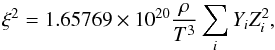 (A.4)
(A.4)
with the numerical factor in agreement with Friedland’s code,
axioncsi= 1.658d20*axionz2ye*Rho/T**3.
Combining
Eq. (
A.2
) and (
A.3
), we obtain
 (A.5)
This
is equivalent to Eq. (
3
), without the artificial
ρ
dependence,
now only present in
f(ξ2)
.
With
T
in
K, it gives
(A.5)
This
is equivalent to Eq. (
3
), without the artificial
ρ
dependence,
now only present in
f(ξ2)
.
With
T
in
K, it gives
 (A.6)
again
with a numerical factor in agreement with Friedland’s code,
(A.6)
again
with a numerical factor in agreement with Friedland’s code,
4.66d-31*axionz2ye*faxioncsi*axion_g10**2*T**4.
For
a homogeneous composition (
 ),
the sum appearing in these equations
),
the sum appearing in these equations
 is
just equal to
Z/A + Z2/A,
where
the first and second term corresponds to the electron and ion contribution, respectively. This gives a factor of e.g. 2 for pure
1
H
or 3/2 for pure
4
He.
However,
Friedland et al. (2013
)
used for this sum
is
just equal to
Z/A + Z2/A,
where
the first and second term corresponds to the electron and ion contribution, respectively. This gives a factor of e.g. 2 for pure
1
H
or 3/2 for pure
4
He.
However,
Friedland et al. (2013
)
used for this sum
ye = zbar * abari
axionz2ye=z2bar+ye,
which
translates into
 (Mads
Soerensen priv. comm.). The sum would then be calculated incorrectly, e.g. 4+2/4 instead of 6/4 for pure
4
He,
i.e. a factor of 3 difference, which will increase during subsequent burning phases.
(Mads
Soerensen priv. comm.). The sum would then be calculated incorrectly, e.g. 4+2/4 instead of 6/4 for pure
4
He,
i.e. a factor of 3 difference, which will increase during subsequent burning phases.
All Tables
Masses of the helium and carbon-oxygen cores at the end of the core C-burning phase.
All Figures
|
Fig. 1 Primakoff effect: a real photon from the thermal bath is converted into an axion by the electric field of a nucleus. |
| In the text | |
|
Fig. 2 Hertzsprung-Russell diagram for the six models computed at solar metallicity. Dashed lines show models without axion losses. Solid lines show models with axion losses. Circles (without axion losses) and squares (with axion losses) show the location of the models at the end of core He-burning. Blue crosses show the location of the tracks at core helium-burning ignition (ϵ(3α) > 0). |
| In the text | |
|
Fig. 3 Same as Fig. 2, but for the 16 Pop. III models. The shaded area shows the zone of the diagram where helium burns in the core of the models without axion losses. The thin black line shows the location of the models without axion losses when the carbon starts to burn into the core. The shaded area and the black line are similar for models with axion losses. Circles (without axion losses) and squares (with axion losses) show the location of the models at the end of core C-burning. |
| In the text | |
|
Fig. 4 Relative difference of the duration of MS and core helium-burning phases between Pop. III models with (g10 = 1, noted as g1) and without (g10 = 0, noted as g0) axion losses. |
| In the text | |
|
Fig. 5 Coloured lines shows the tracks for the computed Pop. III models in the central temperature vs. central density plane. Dashed lines show models without axion losses, while solid lines show models with axion losses. The ignition of the different burning stages and the end of central helium burning are given for the models without axion losses. The broad dashed Γ < 4 / 3 line indicates the zone of the diagram where electron-positron pair creations lower the adiabatic index below 4/3. The X = 1 and Z = 1 lines show the limit between the perfect gas and the completely degenerate non-relativistic gas for pure hydrogen and pure metal mixtures. Light purple lines delimitate the different regions where a given neutrino source (pair, photoneutrino, bremsstrahlung, and plasma) dominates. The colour map shows the ratio ϵax/ϵν , where ϵν is the sum of the four types of neutrino losses mentioned above, computed according to Itoh et al. (1989, 1996). |
| In the text | |
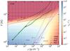 |
Fig. 6 Same as Fig. 5, but for the 85 and 120 M⊙ models. |
| In the text | |
|
Fig. 7 Energy generated by helium burning (ϵHe), carbon burning (ϵC), gravitational energy (ϵgrav), energy of the neutrinos (ϵν), and of the axions (ϵax). Thick lines represent sources of energy, and thin lines represent sinks of energy. The dotted line shows the ratio ϵax / ϵν. The vertical dashed line denotes the end of the core helium-burning phase. |
| In the text | |
|
Fig. 8 ϵax/ϵν ratio in the core of Pop. III models as a function of the time after the end of central helium burning. |
| In the text | |
|
Fig. 9 Kippenhahn diagram of the 85g0 (left) and 85g1 (right) models. Grey areas represent the convective zones. The red line at the top shows the total mass. The core hydrogen-, helium-, and carbon-burning phases are indicated at the top of the panels. |
| In the text | |
|
Fig. 10 Ratio of central abundances at the end of core C-burning between models with axion losses ( |
| In the text | |
|
Fig. 11 Abundance profiles of the 85g0 (left) and 85g1 (right) models at the end of core carbon burning (central mass fraction of 12C below 10-5). The shaded area shows the convective zones. |
| In the text | |
Current usage metrics show cumulative count of Article Views (full-text article views including HTML views, PDF and ePub downloads, according to the available data) and Abstracts Views on Vision4Press platform.
Data correspond to usage on the plateform after 2015. The current usage metrics is available 48-96 hours after online publication and is updated daily on week days.
Initial download of the metrics may take a while.