© ESO, 2017

1. Introduction

Observing stellar phenomena provides insight into the evolution of matter in the universe. However, these observations are necessarily constrained by the opacity of stellar atmospheres to radiation; we cannot easily probe deep into the cores of stars to directly observe their structure. Stellar models are required to make the connection between observations and the internal structure of stars. Clearly, the accuracy of these models is paramount. To fully investigate the validity of stellar models and compare them with observations, we must account for uncertainties in the physical quantities used as inputs to those models. One such input is the rate at which nuclear reactions occur in stellar environments. Understanding the uncertainties in reaction rates is therefore critical to understanding the internal structure of stars and stellar phenomena.

A large step forward in determining statistically realistic uncertainties of reaction rates was made in Longland et al. (2010) and Iliadis et al. (2010a,b,c). A Monte Carlo method was developed for determining statistically realistic uncertainties of reaction rates taking into account experimental uncertainties. This was then expanded by Sallaska et al. (2013) and Mohr et al. (2014), and summarized in Iliadis et al. (2015) and Champagne et al. (2014). These developments form the basis for the Starlib reaction rate library (starlib.physics.unc.edu). Similar methods have been developed by Rauscher et al. (2016). Briefly, nuclear reaction cross section inputs are represented by probability density distributions, which are then propagated, through Monte Carlo variation, to a probability density distribution of the reaction rate. This final reaction rate distribution is temperature dependent. Unlike more traditional methods that yield “upper” and “lower” limits on reaction rates, this method yields continuous probability functions with a “high” and “low” rate defined by the 68% coverage interval. Once uncertainties of reaction rates are determined, they can be used in stellar models to determine the effect that nuclear physics uncertainties have on nucleosynthesis. It should be stressed here that these uncertainties can be either derived from experimental results or from estimated theoretical uncertainties.

Often, cross sections are dominated by resonances. Hence, the uncertain cross section inputs in reaction rate calculations are resonance strengths, partial width measurements, or resonance energies. These are often not measured absolutely, but are measured with respect to well-known “reference” resonances. Indeed, the first reaction rate compilation based on reference resonances was that of Iliadis et al. (2001). These reference resonances often have appreciable uncertainties of their own, leading to correlated uncertainties in the relative measurements. The nature of the correlation between quantities is often not reported. However, a conservative estimate of this effect can be estimated by comparing the magnitude of measurement uncertainties. For example, if a standard resonance strength is uncertain by 20%, then all subsequent measurements are also uncertain by 20% plus any additional systematic or statistical uncertainty present in their measurement. Those resonance strengths are correlated. Accounting for this effect has, so far, not been included in the Monte Carlo reaction rate formalism discussed above. Here, an extension to that method is described that allows correlated uncertainties to be taken into account in reaction rate calculations.

This paper is organized as follows: an introduction to the Monte Carlo reaction rate formalism is presented in Sect. 2 before the addition of correlated uncertainties is discussed in Sect. 3. The correlation formalism for Monte Carlo reaction rates is developed in Sect. 3.1. Four test cases are used to investigate the impact of these effects on nucleosynthesis models. Their results are discussed in Sect. 4, and conclusions are presented in Sect. 5.

2. Monte Carlo reaction rates

The reaction rate per particle pair, ⟨ σv ⟩, is defined as $\mathrm{⟨}\mathit{\sigma v}\mathrm{⟩}\mathrm{=}{\left(\frac{\mathrm{8}}{\mathit{\pi \mu }}\right)}^{\mathrm{1}\mathit{/}\mathrm{2}}\frac{\mathrm{1}}{\mathrm{(}{\mathit{k}}_{\mathrm{B}}\mathit{T}{\mathrm{)}}^{\mathrm{3}\mathit{/}\mathrm{2}}}{\mathrm{\int }}_{\mathrm{0}}^{\mathrm{\infty }}\mathit{E\sigma }\mathrm{\left(}\mathit{E}\mathrm{\right)}{\mathrm{e}}^{\mathrm{-}\mathit{E}\mathit{/}{\mathit{k}}_{\mathit{B}}\mathit{T}}\mathrm{d}\mathit{E,}$(1)where μ is the reduced mass of the system, k_B is the Boltzmann constant, T is the temperature at which the reaction rate is being calculated, and σ(E) is the energy-dependent cross section of the reaction. Many reactions of astrophysical importance proceed through nuclear resonances, populating compound nuclear states that subsequently decay. For a single, isolated resonance, the cross section in Eq. (1) can be replaced by $\mathit{\sigma }\mathrm{\left(}\mathit{E}\mathrm{\right)}\mathrm{=}\frac{\mathrm{2}\mathit{J}\mathrm{+}\mathrm{1}}{\mathrm{(}\mathrm{2}{\mathit{J}}_{\mathrm{1}}\mathrm{+}\mathrm{1}\mathrm{)}\mathrm{(}\mathrm{2}{\mathit{J}}_{\mathrm{2}}\mathrm{+}\mathrm{1}\mathrm{)}}\frac{\mathit{\pi }}{{\mathit{k}}_{\mathrm{B}}^{\mathrm{2}}}\frac{{\mathrm{\Gamma }}_{\mathit{a}}\mathrm{\left(}\mathit{E}\mathrm{\right)}{\mathrm{\Gamma }}_{\mathit{b}}\mathrm{\left(}\mathit{E}\mathrm{\right)}}{\mathrm{(}\mathit{E}\mathrm{-}{\mathit{E}}_{\mathit{r}}{\mathrm{)}}^{\mathrm{2}}\mathrm{+}{\mathrm{\Gamma }}^{\mathrm{2}}\mathit{/}\mathrm{4}}\mathrm{·}$(2)Here, J, J₁, and J₂ are the spins of the resonance, target, and projectile particles, respectively. Γ_a and Γ_b are energy-dependent quantities describing the particle and reaction partial widths of the state in question. For example, for a (p, γ) reaction, Γ_a corresponds to the proton partial width and Γ_b is the γ-ray partial width. Γ corresponds to the total width of the state, and E_r is the resonance energy. These parameters are often determined experimentally using a wide variety of experimental techniques of differing precision. Some experimental methods are best suited to measuring the integrated cross section across narrow resonances. In that case, we refer to a resonance strength, ωγ, and Eq. (1) is replaced with $\mathrm{⟨}\mathit{\sigma v}\mathrm{⟩}\mathrm{=}{\left(\frac{\mathrm{2}\mathit{\pi }}{\mathit{\mu }{\mathit{k}}_{\mathrm{B}}\mathit{T}}\right)}^{\mathrm{3}\mathit{/}\mathrm{2}}{ħ}^{\mathrm{2}}\sum _{\mathit{i}}\mathit{\omega }{\mathit{\gamma }}_{\mathit{i}}{\mathrm{e}}^{\mathrm{-}{\mathit{E}}_{\mathit{r}}\mathit{/}{\mathit{k}}_{\mathit{B}}\mathit{T}}\mathit{.}$(3)This paper focuses on reaction rates dominated by resonances in the absence of interference. Addressing interfering resonance reaction rates that are best described by R-matrix or other complex models is left for future work.

Each of the partial widths, resonance strengths, and resonance energies described by Eqs. (2) and (3) has some associated uncertainty. These are used as inputs to calculate reaction rate. The general strategy for using Monte Carlo uncertainty propagation of reaction rates is as follows: (i) generate random variables corresponding to each uncertain input by varying them according to their experimental uncertainties, (ii) calculate the reaction rate at each temperature, and (iii) repeat many (10 000) times. Care must be taken during this procedure to correctly propagate resonance energy uncertainties, particularly for wide resonances that are integrated numerically. The resonance energy enters Eq. (2) in multiple places, so this must be taken into account. Following this procedure, an ensemble of reaction rates is obtained that can be summarized using descriptive statistics. Longland et al. (2010) found that two parameters are sufficient to summarize the reaction rate at each temperature, that is, μ and σ, the location and shape parameters of a lognormal distribution. Note that these parameters evolve smoothly as a function of temperature. The recommended reaction rate at temperature T is given by (see Evans et al. 2000; Sallaska et al. 2013) $\mathrm{⟨}\mathit{\sigma v}{\mathrm{⟩}}_{\mathrm{rec}\mathrm{.}}\mathrm{=}{\mathrm{e}}^{\mathit{\mu }\mathrm{\left(}\mathit{T}\mathrm{\right)}}\mathit{,}$(4)and the factor uncertainty, f.u. is defined by $\mathit{f}\mathit{.}\mathit{u}\mathit{.}\mathrm{=}{\mathrm{e}}^{\mathit{\sigma }\mathrm{\left(}\mathit{T}\mathrm{\right)}}\mathit{.}$(5)Additionally, the “low” and “high” rates provided by the 1-σ uncertainties are found using $\mathrm{⟨}\mathit{\sigma v}{\mathrm{⟩}}_{\mathit{l}}\mathrm{=}\mathrm{⟨}\mathit{\sigma v}{\mathrm{⟩}}_{\mathrm{rec}\mathrm{.}}\hspace{0.17em}\mathrm{(}\mathit{f}\mathit{.}\mathit{u}\mathit{.}{\mathrm{)}}^{-1} \mathrm{⟨}\mathit{\sigma v}{\mathrm{⟩}}_{\mathit{h}}\mathrm{=}\mathrm{⟨}\mathit{\sigma v}{\mathrm{⟩}}_{\mathrm{rec}\mathrm{.}}\hspace{0.17em}\mathrm{(}\mathit{f}\mathit{.}\mathit{u}\mathit{.}{\mathrm{)}}^{\mathrm{+}\mathrm{1}}\mathit{.}$(6)Once parameters that describe temperature dependent reaction rates and their uncertainties have been found, Monte Carlo procedures can also be applied to find the effect these uncertainties have on nucleosynthesis in stars. Techniques for using the temperature-dependent recommended rate and factor uncertainty parameters in nucleosynthesis calculations were first investigated in Longland (2012). A single, randomly sampled temperature-dependent parameter, p(T), was found to be sufficient for generating reaction rate samples. In fact, it was also found that p(T) need not be temperature dependent for accurate reproduction of nucleosynthesis uncertainties, and must only be normally distributed. Thus, a single reaction rate sample can be represented by $\mathrm{⟨}\mathit{\sigma v}{\mathrm{⟩}}_{\mathit{i}}\mathrm{=}\mathrm{⟨}\mathit{\sigma v}{\mathrm{⟩}}_{\mathrm{rec}\mathrm{.}}\hspace{0.17em}\mathrm{(}\mathit{f}\mathit{.}\mathit{u}\mathit{.}{\mathrm{)}}^{{\mathit{p}}_{\mathit{i}}}\mathit{.}$(7)Monte Carlo nucleosynthesis calculations can be performed using this scheme by generating an ensemble of standard normally distributed p_i values for each reaction. As long as those values are retained for each nucleosynthesis calculation, techniques can be developed to characterize which reaction rate uncertainties most affect model predictions of nucleosynthesis. Most of these methods consist of calculating the correlation between the final abundance of a particular isotope with the p_i values of a reaction rate. A few of those techniques have already been investigated by Iliadis et al. (2015), and further methods are forthcoming. It should be stressed, here, that these p_i values represent variations of a reaction within its experimental or theoretical uncertainty. Section 4 relies on these Monte Carlo nucleosynthesis techniques to investigate the impact of correlated nuclear inputs on nucleosyhtnesis predictions in stellar modes. For the sake of clarity, only the reaction in question and its reverse reaction are varied, holding all other reactions at their recommended rates.

As mentioned, the first step in the procedure to calculate Monte Carlo reaction rate uncertainties is to generate random variables for all input parameters. This step provides us with an opportunity to account for input parameter correlations. Procedures already exist for generating correlated random numbers and are laid out in Sect. 3.1, but first the source and behavior of those correlations should be determined.

3. Correlated uncertainties in reaction rates

Resonance strengths can be measured directly. A solid substrate containing the target of interest is usually constructed, and bombarded by a beam of particles corresponding to the incoming channel. Note that the concepts outlined in this section are equally applicable to inverse kinematics experiments. The reaction yield is then measured using some detection scheme. For example, a high intensity proton beam can be used in conjunction with γ-ray detectors to measure proton radiative capture reactions. To determine a single resonance strength, the beam energy is tuned such that the beam particles lose energy as they traverse the target, thus effectively integrating the cross section (a more in-depth discussion of these techniques can be found in Rolfs & Rodney 1988 and Iliadis 2015). The resonance strength, ωγ, is determined by $\mathit{\omega \gamma }\mathrm{=}\frac{\mathrm{2}{\mathit{\epsilon }}_{\mathit{r}}}{{\mathit{\lambda }}_{\mathit{r}}^{\mathrm{2}}}\frac{\mathit{N}}{{\mathit{N}}_{\mathit{b}}\mathit{B\eta W}}\mathit{,}$(8)where ε_r is the stopping power of the target (usually replaced by ε_eff if the target is a compound substrate) and λ_r is the deBroglie wavelength at the resonance energy. The quantities N and N_b denote the number of detected products (γ-rays in this case) and number of beam particles (protons), respectively. B is the branching ratio of the detected reaction product, η is the detection efficiency, and W is a quantity that takes into account any angular-dependent effects in the reaction. Every one of these parameters is uncertain to some degree. The uncertainty in a resonance strength is therefore computed from the product of random variables. The Central Limit Theorem tells us that the uncertainty in this product will be distributed according to a lognormal distribution. This concept and its impact on nuclear reaction rate uncertainties is described in more detail by Longland et al. (2010).

To determine a resonance strength absolutely, target material properties must be known to a high degree of accuracy. Beam current and absolute detector efficiencies must be similarly well known. To avoid these constraints, however, one can turn to relative measurements. Here, a resonance strength measurement is normalized to a well known resonance that was measured, separately, using a carefully calibrated system. That resonance – referred to here as a reference resonance and denoted herein with a subscript “r” – is then used to normalize subsequent measurements. Absolute determination of beam current, detector efficiency, and target properties can then be canceled in Eq. (8). The consequence of this procedure is that those subsequent resonance strengths are correlated with the reference resonance. Furthermore, their uncertainties are necessarily larger than the reference strength uncertainty. This fact is crucial to the correlation technique described below. For example, Powell et al. (1998) measured the strength of the ${\mathit{E}}_{\mathit{r}}^{\mathrm{lab}}\mathrm{=}\mathrm{406}$ keV resonance in ²⁷Al(p, γ)²⁸Si with an uncertainty of σ_r = 6.0%. Any subsequent relative resonance strength measurement in the same reaction will contain an uncertainty ${\mathit{\sigma }}^{\mathrm{2}}\mathrm{=}{\mathit{\sigma }}_{\mathit{j}}^{\mathrm{2}}\mathrm{+}{\mathit{\sigma }}_{\mathit{r}}^{\mathrm{2}}\mathit{,}$(9)where σ_j comprises of any uncertainty in the relative measurement that cannot be cancelled out in Eq. (8). Any remaining factors affecting the uncertainty in resonance j will, therefore, be independent of resonance r. Equation (9) dictates that all normalized resonances must have larger uncertainties than the reference. This also gives us a convenient method for identifying the reference resonance when such information is not clearly presented: the reference resonance will always contain the smallest uncertainties.

Similar arguments can be made for partial width determinations. Often, if a partial width is determined based on a spectroscopic factor or asymptotic normalization coefficient (ANC), normalization to a well known reference resonance is performed. In the interest of clarity, the following discussion will only refer to reaction rates that are dominated by narrow resonance strengths.

3.1. Monte Carlo treatment of correlated uncertainties

To demonstrate the generation of correlated Monte Carlo uncertainties in resonance strengths for reaction rate calculations, we first consider correlated random variables represented by the vector, x^′. Assuming, for now, that x^′ is distributed according to a multivariate probability density function characterized by mean values of μ and standard deviations of σ, we can write ${\mathit{P}}_{{{x}}^{{\prime }}}\mathrm{=}\frac{\mathrm{1}}{\sqrt{\mathrm{\left(}\mathrm{2}\mathit{\pi }{\mathrm{)}}^{\mathit{k}}\mathrm{\right|}{\Sigma }\mathrm{|}}}\exp \left(\mathrm{-}\frac{\mathrm{1}}{\mathrm{2}}\mathrm{(}{{x}}^{{\prime }}\mathrm{-}{\mu }{\mathrm{)}}^{\mathit{T}}{{\Sigma }}^{-1}\mathrm{(}{{x}}^{{\prime }}\mathrm{-}{\mu }\mathrm{)}\right)\mathit{.}$(10)The matrix, Σ is the covariance matrix, which is assumed to be positive definite and real. Typically, a reaction rate is calculated from the contributions of a large ensemble of resonances. The covariance matrix can therefore be made up of a complex interplay of uncertainties and experimental effects. However, this picture is simplified by realizing that narrow resonance strengths are almost always normalized to a single reference resonance, as already discussed. In this case, the covariance matrix simplifies considerably with no cross correlations. Thus, the uncertainty of each resonance strength is represented by an individual bivariate correlation, but with a different correlation coefficient.

For the bivariate case, x^′ = [ x,y ] and the covariance matrix is defined by ${\Sigma }\mathrm{=}\left[\begin{array}{c}\\ {\mathit{\sigma }}_{\mathit{x}}^{\mathrm{2}}& \mathit{\rho }{\mathit{\sigma }}_{\mathit{x}}{\mathit{\sigma }}_{\mathit{y}}\\ \mathit{\rho }{\mathit{\sigma }}_{\mathit{y}}{\mathit{\sigma }}_{\mathit{x}}& {\mathit{\sigma }}_{\mathit{y}}^{\mathrm{2}}\end{array}\right]\mathrm{=}{{LL}}^{\mathrm{T}}\mathit{,}$(11)where ρ is the correlation coefficient, which varies between 0 and 1; L is a lower triangular matrix with real, positive diagonal entries; and L^T is its conjugate transpose. This decomposition is the so-called Cholesky decomposition, and L can be computed using (Stewart 2000) $\begin{array}{ccc}{\mathit{L}}_{\mathit{jj}}& \mathrm{=}& \sqrt{{\mathrm{\Sigma }}_{\mathit{jj}}\mathrm{-}\sum _{\mathit{k}\mathrm{=}\mathrm{1}}^{\mathit{j}\mathrm{-}\mathrm{1}}{\mathit{L}}_{\mathit{jk}}^{\mathrm{2}}}\mathit{,}\\ {\mathit{L}}_{\mathit{ij}}& \mathrm{=}& \frac{\mathrm{1}}{{\mathit{L}}_{\mathit{jj}}}\left({\mathrm{\Sigma }}_{\mathit{ij}}\mathrm{-}\sum _{\mathit{k}\mathrm{=}\mathrm{1}}^{\mathit{j}\mathrm{-}\mathrm{1}}{\mathit{L}}_{\mathit{ik}}{\mathit{L}}_{\mathit{jk}}\right)\mathit{,} \mathrm{for}\mathit{i}\mathit{>}\mathit{j}\mathit{.}\end{array}$For Eq. (11), L becomes ${L}\mathrm{=}\left[\begin{array}{c}\\ {\mathit{\sigma }}_{\mathit{x}}& \mathrm{0}\\ \mathit{\rho }{\mathit{\sigma }}_{\mathit{x}}& {\mathit{\sigma }}_{\mathit{y}}\sqrt{\mathrm{1}\mathrm{-}{\mathit{\rho }}^{\mathrm{2}}}\end{array}\right]\mathrm{·}$(14)This Cholesky decomposition is useful because it can be used in Monte Carlo calculations to convert uncorrelated normally distributed random variables, x, into correlated quantities, x^′, by (Rubinstein & Kroese 2011) ${{x}}^{{\prime }}\mathrm{=}\mathit{L}{x}\mathit{.}$(15)Equations (15) and (14) can be applied to our bivariate case. Here, we make the additional simplifying assumption that our variables are standardized. That is, σ_x = σ_y = 1. In the discussion above, the concept of reference resonances was discussed. Here, we introduce that concept into our mathematical description of correlated Monte Carlo reaction rates. In the following, the parameter x represents the reference resonance, and y is the other resonance in question that has been normalized to that reference. For sample i of resonance j, therefore, we obtain ${\mathit{y}}_{\mathit{j,i}}^{\mathrm{\prime }}\mathrm{=}{\mathit{\rho }}_{\mathit{j}}{\mathit{x}}_{\mathit{i}}\mathrm{+}\sqrt{\mathrm{1}\mathrm{-}{\mathit{\rho }}_{\mathit{j}}^{\mathrm{2}}}\hspace{0.17em}\hspace{0.17em}{\mathit{y}}_{\mathit{j,i}}\mathit{.}$(16)Why assume σ = 1? Often in statistical procedures, particularly those involving Monte Carlo computation, it is convenient to standardize parameters to avoid scale effects. It is trivial to un-standardize the random variables following their computation in Eq. (16). For example, since resonance strengths are random variables described by a lognormal probability density distribution as discussed above, Monte Carlo samples of a resonance strength, ωγ_j, can be described in the same way as the reaction rate in Eq. (7) by $\mathit{\omega }{\mathit{\gamma }}_{\mathit{j,i}}\mathrm{=}\mathit{\omega }{\mathit{\gamma }}_{\mathit{j,}\mathrm{rec}\mathrm{.}}\hspace{0.17em}\mathrm{(}\mathit{f}\mathit{.}\mathit{u}\mathit{.}{\mathrm{)}}^{{\mathit{y}}_{\mathit{j,i}}^{\mathrm{\prime }}}$(17)where ωγ_j,rec. is the recommended resonance strength, and f.u. is its factor uncertainty. The quantity ${\mathit{y}}_{\mathit{j,i}}^{\mathrm{\prime }}$ is a standard, normally distributed, correlated random variable calculated in Eq. (16). To fully describe correlated resonance strengths, therefore, one only needs to compute the values ${\mathit{y}}_{\mathit{j,i}}^{\mathrm{\prime }}$ using Eq. (16).

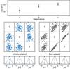Fig. 1 Example of correlated Monte Carlo samples. Top panel: strengths of our three example resonances including their uncertainties. Middle panel: uncorrelated (blue – yj) and correlated (grey – ${\mathit{y}}_{\mathit{j}}^{\mathrm{\prime }}$) normally distributed samples, which are used to compute the resonance strengths in Eq. (17). Note that after applying the correlation outlined in the text, resonances 2 and r become highly correlated whereas resonance one remains largely unchanged. Lower two panels: density distributions of the samples, and confirms that the individual distributions do not vary outside of statistical fluctuations.

The remaining challenge is to determine the correlation parameters, ρ_j, for each resonance. In the absence of information, it would be pertinent to assume, conservatively, that resonances are maximally correlated. We cannot, however, simply use ρ = 1. Recall that any normalized quantity must have larger uncertainties than the reference resonance. Therefore, the correlation parameter for each resonance strength is calculated by the ratio of their fractional uncertainties: ${\mathit{\rho }}_{\mathit{j}}\mathrm{=}\frac{{\mathit{\sigma }}_{\mathit{r}}}{\mathit{\omega }{\mathit{\gamma }}_{\mathit{r}}}\frac{\mathit{\omega }{\mathit{\gamma }}_{\mathit{j}}}{{\mathit{\sigma }}_{\mathit{j}}}\mathrm{=}\frac{\mathit{f}\mathit{.}\mathit{u}{\mathit{.}}_{\mathit{r}}}{\mathit{f}\mathit{.}\mathit{u}{\mathit{.}}_{\mathit{j}}}\mathrm{·}$(18)Note that the fractional uncertainties can be simply replaced by the factor uncertainty. When the resonance, j, contains an uncertainty close to the reference, r, its uncertainty is dominated by the uncertainty in the latter and Eq. (18) shows that ρ_j → 1. Furthermore, as statistical and other uncorrelated uncertainties begin to dominate resonance strengths, their uncertainties become much larger than those of the reference strength and ρ becomes small. Under this set of assumptions, it’s also impossible for ρ to exceed unity.

The general procedure for calculating correlated reaction rate uncertainties from narrow resonance strengths is therefore as follows: (i) identify the reference resonance, r by assuming it is the resonance with the smallest fractional uncertainty; (ii) calculate the correlation parameters for all other resonance strengths using Eq. (18); (iii) generate a set of standard normally distributed random variables, y_j,i for each resonance; (iv) correlate those using Eq. (16) to obtain ${\mathit{y}}_{\mathit{j,i}}^{\mathrm{\prime }}$; (v) calculate an ensemble of correlated resonance strengths using Eq. (17); and (vi) compute the reaction rate for each set of samples. The ensemble of reaction rates from this procedure can be summarized to find a recommended rate, “High” and “Low” rates, and shape parameters μ and σ using the procedures discussed in Longland et al. (2010).

4. Results and discussion

To investigate the effects of correlated cross section uncertainties on reaction rates, a few cases are considered. A simple example reaction consisting of three resonances will be used to illustrate the procedure, followed by ²⁷Al(p, γ)²⁸Si and two examples of reactions on ²³Na: ²³Na(p, α)²⁰Ne and ²³Na(α, p)²⁶Mg.

4.1. Simple example

To illustrate the procedure of generating correlated uncertainties in Monte Carlo reaction rates, consider a fictional reaction consisting of three resonances with strengths ωγ₁, ωγ₂, and the reference resonance, ωγ_r. The strengths of the first two resonances are normalized to the reference resonance and we assume that their uncertainties have been correctly computed to account for that. Details of their energies and resonance strengths can be found in Table 1, and are plotted in the top panel of Fig. 1. The resonance strengths all have different uncertainties owing to expected experimental constraints. The weaker resonance, for example, has a large uncertainty arising mostly from counting statistics. Inspection of the uncertainties, therefore, immediately reveals that resonance 2 is highly correlated with the reference resonance, whereas resonance 1 is dominated by low statistics, and is therefore less correlated. The correlation factors calculated from Eq. (18) reflect these arguments.

The procedure outlined in Sect. 3.1 is performed, and shown in the middle row of Fig. 1. The uncorrelated values, y_j,i are generated and shown in the left-middle panel in a “pairs plot”: a scatterplot matrix showing the bivariate relationships between the resonance strengths (Hartigan 1975). The correlated values calculated from Eq. (16) using the correlation parameters listed in Table 1 are displayed in the right-side pairs plot. It is immediately apparent that the Monte Carlo samples for resonance 2 become highly correlated with the reference resonance, but there is only weak correlation for resonance 1. Note, also, that the probability density distributions for individual parameters remain unchanged following the correlation procedure, as shown in the bottom row of Fig. 1. This is an important validation; the uncertainties of individual resonances should not be affected by this procedure, only their inter-dependence. Finally, correlated samples of resonance strengths are calculated using Eq. (17). Each set of sampled strengths is used to compute a sample reaction rate at temperature, T using Eq. (3). The resulting rate uncertainties are presented later in Sect. 4.

The reaction rate uncertainties for the simple 3-resonance reaction are shown in Fig. 2. For clarity, the uncertainties are normalized to the recommended rate. A value of 2.0, for example, corresponds to a rate that is twice the recommended rate. At low temperatures, the rate is dominated by resonance 1 and the reaction rate probability distribution is largely unchanged following the correlation procedure. At high temperatures above about 200 MK, correlation between resonances 2 and r becomes important. The grey uncertainty band representing correlated rates is clearly wider than the blue, uncorrelated rate uncertainties. Even at higher temperatures, though, the rate uncertainties don’t increase significantly, despite the strong correlation between resonances 2 and r. This is a consequence of the relative strength of the two resonances. The latter resonance dominates the rate at high temperatures, contributing roughly 60% with the other two resonances only contributing 30% (resonance 2) and 10% (resonance 1).

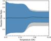Fig. 2 Reaction rate uncertainties as a function of temperature and normalized to the recommended rate. The blue shaded region shows the uncorrelated 1 − σ uncertainties of the rate, while the grey region represents rate uncertainties once correlated uncertainties are taken into account. Clearly, at low temperatures where the rate is dominated by only one resonance, there is no difference in the reaction rate uncertainties when applying this procedure.

4.2. ²⁷Al(p, γ)²⁸Si

The ²⁷Al(p, γ)²⁸Si reaction is of astrophysical importance, strongly influencing the rate of ²⁷Al production in stellar environments by affecting the leakage of material out of the AlMg cycle in massive stars (Prantzos & Diehl 1996; Harissopulos et al. 2000; Powell et al. 1998). Its long recognized importance has lead to numerous experimental resonance strength studies, most recently those of Powell et al. (1998), Chronidou et al. (1999), and Harissopulos et al. (2000). The former of these results has been used in Iliadis et al. (2010c) to normalize other experimental resonance strength determinations, thus introducing correlation between these parameters. Furthermore, experimental information for this reaction reaches high enough energies that theoretical Hauser-Feshbach rates are not required to supplement the experimental information at high temperatures. Here, we use the same input parameters as those in Iliadis et al. (2010a), so the reader is referred to that publication for details.

Although the resonance density of the ²⁷Al(p, γ)²⁸Si reaction is high, the low-energy resonances that dominate the reaction rate below 100 MK are poorly known and therefore are not strongly correlated with the reference resonance at ${\mathit{E}}_{\mathit{r}}^{\mathrm{c}\mathit{.}\mathrm{m}\mathit{.}}\mathrm{=}\mathrm{391.3}$ keV measured by Powell et al. (1998). Thus, the reaction rate uncertainties at temperatures below 100 MK are largely unchanged when correlations are taken into account. This is reflected in Fig. 3. However, at high temperatures, where there are many contributing resonances that are correlated with the reference resonance, we see the reaction rate uncertainties increase by up to a factor of 2.5.

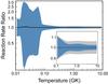Fig. 3 Reaction rate uncertainty comparison for the 27Al(p, γ)28Si reaction when including resonance strength correlations. Correlations only affect the reaction rate uncertainties at temperatures above 300 MK. This is because at lower temperatures, the reaction rate is dominated by only a few resonances at 72 keV, 84 keV, and 196 keV.

The ²⁷Al(p, γ)²⁸Si reaction primarily affects leakage of material out of the Mg-Al cycle and strongly determines the synthesis of ²⁷Al in massive stars (Prantzos & Diehl 1996; Harissopulos et al. 2000; Powell et al. 1998). In these environments, temperatures are restricted to T< 90 MK. For the sake of the present study, we consider a single-zone model based on the core hydrogen-burning parameters shown in Cavallo et al. (1998). That is: T = 50 MK and ρ = 600 g/cm³. It is clear, from inspection of Fig. 3, that the rate uncertainties for this reaction at 50 MK are unchanged when taking correlations into account. Therefore, nucleosynthesis (namely the destruction of ²⁷Al in the environment) in this case is unaffected by correlation effects.

4.3. ²³Na(p, α)²⁰Ne

The ²³Na(p, α)²⁰Ne reaction is of key importance in understanding the destruction of ²³Na needed to explain abundance anomalies in globular clusters (Gratton et al. 2004; Hale et al. 2004; Cesaratto et al. 2013). The destruction of sodium requires high temperature hydrogen burning, such as the shell burning found in massive AGB stars (Ventura et al. 2001; D’Antona et al. 2002; Denissenkov & Herwig 2003), rotating massive AGB stars (Decressin & Charbonnel 2005), rotating massive stars (Prantzos & Charbonnel 2006; Decressin et al. 2007), or massive binaries (de Mink et al. 2009).

Recent experimental results (Cesaratto et al. 2013) for the competing ²³Na(p, γ)²⁴Mg reaction showed that the main source of nucleosynthesis uncertainty for ²³Na now comes from the (p,α) reaction’s cross section. We should also note, here, that there is a mistake in the reaction rate input for this reaction presented on page 281 of Iliadis et al. (2010a). The resonance at ${\mathit{E}}_{\mathit{r}}^{\mathrm{c}\mathit{.}\mathrm{m}\mathit{.}}\mathrm{=}\mathrm{-}\mathrm{303.0}$ keV was found in Hale et al. (2002) to have a spectroscopic factor of C²S = 0.02. Combining that with the single particle reduced width of ${\mathit{\theta }}_{\mathrm{sp}}^{\mathrm{2}}\mathrm{=}\mathrm{0.6}$ from Iliadis (1997) yields a reduced width θ² = 0.012, in contradiction with the value found in Iliadis et al. (2010a). We will therefore use this updated value in the calculations below. The sub-threshold resonance at ${\mathit{E}}_{\mathit{r}}^{\mathrm{c}\mathit{.}\mathrm{m}\mathit{.}}\mathrm{=}\mathrm{-}\mathrm{303.0}$ keV now has a negligible contribution to the reaction rate at all temperatures, which lowers the rate by approximately 10% at T = 0.01–0.06 GK. All other inputs are the same as those found in Iliadis et al. (2010a).

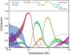Fig. 4 Fractional contributions of individual resonances and sub-threshold resonances to the 23Na(p, α)20Ne reaction rate. The bands shown account for the uncertainties in each resonance’s input parameters.

This reaction is rather more complex than the previous examples. It consists of a number of directly measured resonances above ${\mathit{E}}_{\mathit{r}}^{\mathrm{c}\mathit{.}\mathrm{m}\mathit{.}}\mathrm{=}\mathrm{217}$ keV, but also includes resonances and sub-threshold resonances whose widths have been determined by some other means, namely particle transfer measurements (Hale et al. 2004; Fuchs et al. 1968). We will assume here that the model uncertainties in those measurements (Iliadis et al. 2010a, uses a standard value of 40%) are correlated only by normalization to higher energy resonances. Cross correlation between these transfer results would arise from model effects, but these effects may affect states differently, depending on their single-particle nature. The sub-threshold resonances dominate the reaction rate at temperatures below 40 MK while the two broad resonances at ${\mathit{E}}_{\mathit{r}}^{\mathrm{c}\mathit{.}\mathrm{m}\mathit{.}}\mathrm{=}\mathrm{170}$ keV and ${\mathit{E}}_{\mathit{r}}^{\mathrm{c}\mathit{.}\mathrm{m}\mathit{.}}\mathrm{=}\mathrm{274}$ keV dominate the rate between 40 MK and about 500 MK. Fractional contributions to the rate are more readily visualized in Fig. 4. Care should be taken in interpreting these contribution plots. For example, while the ${\mathit{E}}_{\mathit{r}}^{\mathrm{c}\mathit{.}\mathrm{m}\mathit{.}}\mathrm{=}\mathrm{170}$ keV resonance is rather uncertain (20% uncertainty in the proton width), its contribution to the total reaction rate at 100 MK is well constrained at the 1% level. The uncertainty in the total rate is therefore dominated by this single resonance at 100 MK (i.e., 20% uncertainty). We expect the rate uncertainty from correlations to vary significantly according to temperature in this case.

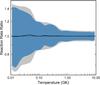Fig. 5 Reaction rate uncertainty comparison for the 23Na(p, α)20Ne reaction. The blue and grey shaded regions correspond to the 1 − σ reaction rate uncertainty bands for the uncorrelated and correlated Monte Carlo reaction rate calculations, respectively.

The rate of the ²³Na(p, α)²⁰Ne reaction is dominated by overlapping wide resonances at low temperatures. We expect larger rate uncertainties if correlations are accounted for, as is reflected in Fig. 5. When correlations are taken into account at 30 MK, the rate uncertainties increase by 33%. On the other hand, at 1 GK where only one resonance at ${\mathit{E}}_{\mathit{r}}^{\mathrm{c}\mathit{.}\mathrm{m}\mathit{.}}\mathrm{=}\mathrm{567}$ keV dominates, the rate uncertainties are largely unchanged. These results have been matched to Hauser-Feshbach theoretical rates at 3.5 GK using the procedure outlined in Newton et al. (2008).

Accounting for correlations in reaction rates is crucial, especially at temperatures where multiple resonances contribute similar fractions of the reaction rate. This is the case at 150 MK where the rate is dominated by two wide resonance at ${\mathit{E}}_{\mathit{r}}^{\mathrm{c}\mathit{.}\mathrm{m}\mathit{.}}\mathrm{=}\mathrm{170}$ keV and ${\mathit{E}}_{\mathit{r}}^{\mathrm{c}\mathit{.}\mathrm{m}\mathit{.}}\mathrm{=}\mathrm{274}$ keV (see Fig. 4). These resonances have comparable uncertainties in their proton partial widths and are normalized to a common reference resonance (Zyskind et al. 1981). If the resonances were allowed to vary independently, their interplay would cause smaller uncertainties at 0.15 GK as shown in blue (essentially, the Monte Carlo variations in each resonance partially cancel each other out). Since these resonances are normalized to a common reference, they should co-vary under Monte Carlo calculations (i.e., as one increases, so should the other). By properly taking correlations into account, this artefact is removed. The correlated uncertainty band shown in grey in Fig. 5 indicates that the method presented here better accounts for the rate uncertainty for multiple contributing resonances.

Whether correlation effects change nucleosynthesis predictions depends strongly on the model in question. For example, shell hydrogen burning in a 5 M_⊙ AGB star with metalicity z = 10^-3 (Ventura & D’Antona 2005) occurs at about 90–100 MK. The rate at this temperature is dominated by the ${\mathit{E}}_{\mathit{r}}^{\mathrm{c}\mathit{.}\mathrm{m}\mathit{.}}\mathrm{=}\mathrm{170}$ keV resonance, hence nucleosynthesis uncertainties are largely unaffected. If another model operated at higher temperatures where correlations do have an effect, we could expect nucleosynthesis prediction uncertainties to increase by up to 30%.

4.4. ²³Na(α, p)²⁶Mg

The ²³Na(α, p)²⁶Mg reaction was shown to be important for ²⁶Al production during C/Ne convective shell burning in massive stars (Iliadis et al. 2011). The critical temperature region identified by for ²⁶Al production in C/Ne convective shell burning is 1.25 GK. The reaction is an important proton source necessary for the ²⁵Mg(p, γ)²⁶Al reaction to proceed. It is also important for the production of ²⁷Al, whose abundance is critical in aluminium isotopic ratio measurements.

This reaction has been studied directly by Kuperus et al. (1963) and Whitmire & Davids (1974) and subsequently in inverse kinematics by Almaraz-Calderon et al. (2014), Tomlinson et al. (2015), Howard et al. (2015), and Avila et al. (2016). The latter studies were not performed with high enough resolution to distinguish individual resonances, and will therefore be discarded for the sake of this illustrative example. Note, though, that the latter studies supersede the forward reaction studies as Iliadis et al. (2011) outlined: target deterioration effects were not properly taken into account in earlier studies. Comparing the reaction rates determined from the normal and inverse kinematics studies suggests that the target effects in Kuperus et al. (1963) and Whitmire & Davids (1974) amount to about 37%.

The α-particle and proton separation energies for this reaction are 10.092 MeV and 8.271 MeV, respectively. The large Q-values mean that it proceeds through higher lying states, so we expect a high level density. Indeed, the average resonance spacing found by Kuperus et al. (1963) and Whitmire & Davids (1974) is about 30 keV. Here, we use the values quoted in those studies with no correction or renormalization applied. The studies are, however, self-normalized. In this case, we expect many resonances to contribute to the reaction rate at any given temperature, so correlations between their strengths will be crucial.

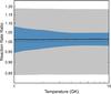Fig. 6 Reaction rate uncertainty comparison for the 23Na(α, p)26Mg reaction. The blue and grey shaded regions correspond to the 1 − σ reaction rate uncertainty bands for the uncorrelated and correlated Monte Carlo reaction rate calculations, respectively.

Rate uncertainties for the ²³Na(α, p)²⁶Mg reaction are shown in Fig. 6 for temperatures between 1 GK and 10 GK. In this case, we see a very large effect of correlations on the reaction rate uncertainties, where the correlated uncertainties (shown in grey) are roughly a factor of 3 larger than when the correlations are not properly taken into account (blue). For higher temperatures, where even more resonances contribute to the rate, the correlated uncertainty is up to a factor of 5 larger than the uncorrelated case. This is because many resonances contribute to the reaction rate owing to the high level density. Thus, their experimental correlation is more critical.

The temperature-density profile defined in Iliadis et al. (2011) is used to investigate the effect of correlated uncertainties on aluminium production. In short, a single-zone profile is extracted from the C/Ne convective shell of the 60 M_⊙ massive star model in Limongi & Chieffi (2006). To account for mixing effects, the time axis of this profile is then compressed by a factor of 60 to reproduce the same nucleosynthesis pattern found in the full model. More details can be found in Iliadis et al. (2011). The ²⁶Al/²⁷Al abundance ratio both before and after taking nuclear correlations into effect is shown in Fig. 7.

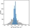Fig. 7 Final 26Al/27Al abundance ratio for the C/Ne convective shell burning profile described in the text. Shown in blue and grey are the final Monte Carlo abundance ratio when considering uncorrelated and correlated reaction rates, respectively.

The abundance ratio in this case is strongly affected by taking correlations in experimental resonance strengths into account when calculating reaction rates. Specifically, the uncertainty in the abundance ratio of ²⁶Al/²⁷Al increases by a factor of 3.5. Clearly, if precise measurements are to be compared with model expectations, these correlation effects must accounted for.

5. Summary

Monte Carlo reaction rate calculations have introduced a new, powerful tool for determining the uncertainties in rates arising from nuclear physics uncertainties. These methods have allowed complex uncertainty propagation to be included without the need for mathematical simplifications, and opened the door for Monte Carlo nucleosynthesis calculations. Before now, no attempt was made to take into account correlations in those nuclear input parameters.

In this paper, the first study aimed at accounting for correlations in resonance strengths and partial widths is presented. By assuming, conservatively, that all resonance strengths or partial widths are normalized to a reference resonance or common experimental systematic error, we are able to compute correlated reaction rate uncertainties with relatively little overhead. This method also establishes a framework for computing correlation parameters in the absence of published correlations. Indeed, in most cases, full covariance data for a measurement is not published, so this conservative estimation provides a safe strategy for flexible application.

Two main lessons can be learned from this investigation: (i) that at low temperatures where most reactions are dominated by only a few resonances, the Monte Carlo reaction rates computed using this method are affected only slightly in comparison to the uncorrelated assumption used previously, and (ii) where many resonances contribute equally to the reaction rate, its uncertainties can increase significantly.

In the future, it would be beneficial to consider the correlation of resonance energies, also. This is particularly useful for radioactive nuclei whose resonance energies are usually determined by subtracting the reaction Q-value. However, it is more challenging in this case to separate different experimental regimes. A few low-energy threshold resonances with large uncertainties may be correlated with each other, but not with a directly measured resonance at high energy.

Correlations between nuclear physics inputs helps us improve our estimates of reaction rate uncertainties that are based on experimental data. While this effect can be minor, it can have dramatic effects on model predictions in certain cases. This study represents a first step to more accurately represent rate uncertainties.

Acknowledgments

The author would like to thank Christian Iliadis, Art Champagne, and Peter Mohr for their comments on the manuscript.

References

All Tables

All Figures

Fig. 1 Example of correlated Monte Carlo samples. Top panel: strengths of our three example resonances including their uncertainties. Middle panel: uncorrelated (blue – yj) and correlated (grey – ${\mathit{y}}_{\mathit{j}}^{\mathrm{\prime }}$) normally distributed samples, which are used to compute the resonance strengths in Eq. (17). Note that after applying the correlation outlined in the text, resonances 2 and r become highly correlated whereas resonance one remains largely unchanged. Lower two panels: density distributions of the samples, and confirms that the individual distributions do not vary outside of statistical fluctuations.

In the text

Fig. 2 Reaction rate uncertainties as a function of temperature and normalized to the recommended rate. The blue shaded region shows the uncorrelated 1 − σ uncertainties of the rate, while the grey region represents rate uncertainties once correlated uncertainties are taken into account. Clearly, at low temperatures where the rate is dominated by only one resonance, there is no difference in the reaction rate uncertainties when applying this procedure.

In the text

	Fig. 3 Reaction rate uncertainty comparison for the 27Al(p, γ)28Si reaction when including resonance strength correlations. Correlations only affect the reaction rate uncertainties at temperatures above 300 MK. This is because at lower temperatures, the reaction rate is dominated by only a few resonances at 72 keV, 84 keV, and 196 keV.
In the text

	Fig. 4 Fractional contributions of individual resonances and sub-threshold resonances to the 23Na(p, α)20Ne reaction rate. The bands shown account for the uncertainties in each resonance’s input parameters.
In the text

	Fig. 5 Reaction rate uncertainty comparison for the 23Na(p, α)20Ne reaction. The blue and grey shaded regions correspond to the 1 − σ reaction rate uncertainty bands for the uncorrelated and correlated Monte Carlo reaction rate calculations, respectively.
In the text

	Fig. 6 Reaction rate uncertainty comparison for the 23Na(α, p)26Mg reaction. The blue and grey shaded regions correspond to the 1 − σ reaction rate uncertainty bands for the uncorrelated and correlated Monte Carlo reaction rate calculations, respectively.
In the text

	Fig. 7 Final 26Al/27Al abundance ratio for the C/Ne convective shell burning profile described in the text. Shown in blue and grey are the final Monte Carlo abundance ratio when considering uncorrelated and correlated reaction rates, respectively.
In the text

References

- Almaraz-Calderon, S., Bertone, P. F., Alcorta, M., et al. 2014, Phys. Rev. Lett., 112, 152701 [NASA ADS] [CrossRef] [PubMed] [Google Scholar]
- Avila, M. L., Rehm, K. E., Almaraz-Calderon, S., et al. 2016, Phys. Rev. C, 94, 065804 [NASA ADS] [CrossRef] [Google Scholar]
- Cavallo, R. M., Sweigart, A. V., & Bell, R. A. 1998, ApJ, 492, 575 [NASA ADS] [CrossRef] [Google Scholar]
- Cesaratto, J., Champagne, A., Buckner, M., et al. 2013, Phys. Rev. C, 88, 065806 [NASA ADS] [CrossRef] [Google Scholar]
- Champagne, A. E., Iliadis, C., & Longland, R. 2014, AIP Adv., 4, 041006 [NASA ADS] [CrossRef] [Google Scholar]
- Chronidou, C., Spyrou, K., Harissopulos, S., Kossionides, S., & Paradellis, T. 1999, Eur. Phys. J. A, 6, 303 [NASA ADS] [CrossRef] [EDP Sciences] [Google Scholar]
- D’Antona, F., Caloi, V., Montalbán, J., Ventura, P., & Gratton, R. 2002, A&A, 395, 69 [NASA ADS] [CrossRef] [EDP Sciences] [Google Scholar]
- de Mink, S. E., Pols, O. R., Langer, N., & Izzard, R. G. 2009, A&A, 507, L1 [NASA ADS] [CrossRef] [EDP Sciences] [Google Scholar]
- Decressin, T., & Charbonnel, C. 2005, in From Lithium to Uranium: Elemental Tracers of Early Cosmic Evolution, eds. V. Hill, P. Francois, & F. Primas, IAU Symp., 228, 395 [Google Scholar]
- Decressin, T., Meynet, G., Charbonnel, C., Prantzos, N., & Ekström, S. 2007, A&A, 464, 1029 [NASA ADS] [CrossRef] [EDP Sciences] [Google Scholar]
- Denissenkov, P. A., & Herwig, F. 2003, ApJ, 590, L99 [NASA ADS] [CrossRef] [Google Scholar]
- Evans, M., Hastings, N., & Peacock, B. 2000, Statistical distributions (Wiley-Interscience) [Google Scholar]
- Fuchs, H., Grabisch, K., Kraaz, P., & Röschert, G. 1968, Nucl. Phys. A, 122, 59 [NASA ADS] [CrossRef] [Google Scholar]
- Gratton, R., Sneden, C., & Carretta, E. 2004, ARA&A, 42, 385 [NASA ADS] [CrossRef] [Google Scholar]
- Hale, S. E., Champagne, A. E., Iliadis, C., et al. 2002, Phys. Rev. C, 65, 015801 [NASA ADS] [CrossRef] [MathSciNet] [Google Scholar]
- Hale, S. E., Champagne, A. E., Iliadis, C., et al. 2004, Phys. Rev. C, 70, 045802 [NASA ADS] [CrossRef] [Google Scholar]
- Harissopulos, S., Chronidou, C., Spyrou, K., et al. 2000, Eur. Phys. J. A, 9, 479 [NASA ADS] [CrossRef] [EDP Sciences] [Google Scholar]
- Hartigan, J. A. 1975, J. Stat. Comput. Simulation, 4, 187 [CrossRef] [Google Scholar]
- Howard, A. M., Munch, M., Fynbo, H. O. U., et al. 2015, Phys. Rev. Lett., 115, 052701 [NASA ADS] [CrossRef] [Google Scholar]
- Iliadis, C. 1997, Nucl. Phys. A, 618, 166 [NASA ADS] [CrossRef] [Google Scholar]
- Iliadis, C. 2015, Nuclear Physics of Stars (John Wiley & Sons) [Google Scholar]
- Iliadis, C., D’Auria, J. M., Starrfield, S., Thompson, W. J., & Wiescher, M. 2001, Astro. Phys. J. S., 134, 151 [Google Scholar]
- Iliadis, C., Longland, R., Champagne, A. E., & Coc, A. 2010a, Nucl. Phys. A, 841, 251 [NASA ADS] [CrossRef] [Google Scholar]
- Iliadis, C., Longland, R., Champagne, A. E., & Coc, A. 2010b, Nucl. Phys. A, 841, 323 [NASA ADS] [CrossRef] [Google Scholar]
- Iliadis, C., Longland, R., Champagne, A. E., Coc, A., & Fitzgerald, R. 2010c, Nucl. Phys. A, 841, 31 [NASA ADS] [CrossRef] [Google Scholar]
- Iliadis, C., Champagne, A., Chieffi, A., & Limongi, M. 2011, ApJS, 193, 16 [Google Scholar]
- Iliadis, C., Longland, R., Coc, A., Timmes, F. X., & Champagne, A. E. 2015, J. Phys. G Nucl. Phys., 42, 034007 [NASA ADS] [CrossRef] [Google Scholar]
- Kuperus, J., Glaudemans, P. W. M., & Endt, P. M. 1963, Physica, 29, 1281 [NASA ADS] [CrossRef] [Google Scholar]
- Limongi, M., & Chieffi, A. 2006, ApJ, 647, 483 [NASA ADS] [CrossRef] [Google Scholar]
- Longland, R. 2012, A&A, 548, A30 [NASA ADS] [CrossRef] [EDP Sciences] [Google Scholar]
- Longland, R., Iliadis, C., Champagne, A. E., et al. 2010, Nucl. Phys. A, 841, 1 [NASA ADS] [CrossRef] [Google Scholar]
- Mohr, P., Longland, R., & Iliadis, C. 2014, Phys. Rev. C, 90, 065806 [NASA ADS] [CrossRef] [Google Scholar]
- Newton, J. R., Longland, R., & Iliadis, C. 2008, Phys. Rev. C, 78, 025805 [NASA ADS] [CrossRef] [Google Scholar]
- Powell, D. C., Iliadis, C., Champagne, A. E., et al. 1998, Nucl. Phys. A, 644, 263 [NASA ADS] [CrossRef] [Google Scholar]
- Prantzos, N., & Charbonnel, C. 2006, A&A, 458, 135 [NASA ADS] [CrossRef] [EDP Sciences] [Google Scholar]
- Prantzos, N., & Diehl, R. 1996, Phys. Rep., 267, 1 [NASA ADS] [CrossRef] [Google Scholar]
- Rauscher, T., Nishimura, N., Hirschi, R., et al. 2016, MNRAS, 463, 4153 [NASA ADS] [CrossRef] [Google Scholar]
- Rolfs, C. E., & Rodney, W. S. 1988, Cauldrons in the Cosmos: Nuclear Astrophysics (University of Chicago Press) [Google Scholar]
- Rubinstein, R. Y., & Kroese, D. P. 2011, Simulation and the Monte Carlo Method (John Wiley & Sons) [Google Scholar]
- Sallaska, A. L., Iliadis, C., Champange, A. E., et al. 2013, ApJS, 207, 18 [NASA ADS] [CrossRef] [Google Scholar]
- Stewart, G. 2000, Comput. Sci. Eng., 2, 50 [CrossRef] [Google Scholar]
- Tomlinson, J. R., Fallis, J., Laird, A. M., et al. 2015, Phys. Rev. Lett., 115, 052702 [NASA ADS] [CrossRef] [Google Scholar]
- Ventura, P., & D’Antona, F. 2005, A&A, 431, 279 [NASA ADS] [CrossRef] [EDP Sciences] [Google Scholar]
- Ventura, P., D’Antona, F., Mazzitelli, I., & Gratton, R. 2001, ApJ, 550, L65 [NASA ADS] [CrossRef] [Google Scholar]
- Whitmire, D. P., & Davids, C. N. 1974, Phys. Rev. C, 9, 996 [NASA ADS] [CrossRef] [Google Scholar]
- Zyskind, J., Rios, M., & Rolfs, C. 1981, ApJ, 243, L53 [NASA ADS] [CrossRef] [Google Scholar]
All Tables
Resonance parameters for example reaction used to demonstrate the effect of correlated uncertainties in resonance strengths on a reaction rate uncertainties.