| Issue |
A&A
Volume 603, July 2017
|
|
|---|---|---|
| Article Number | A109 | |
| Number of page(s) | 10 | |
| Section | The Sun | |
| DOI | https://doi.org/10.1051/0004-6361/201527790 | |
| Published online | 18 July 2017 | |
North-south asymmetry of solar activity as a superposition of two realizations – the sign and absolute value
Pushkov Institute of Terrestrial Magnetism, Ionosphere and Radio Wave Propagation, Russian Academy of Sciences, 108840 Moscow, Troitsk, Russia
e-mail: badalyan@izmiran.ru; obridko@izmiran.ru
Received: 19 November 2015
Accepted: 29 March 2017
Context. Since the occurrence of north-south asymmetry (NSA) of alternating sign may be determined by different mechanisms, the frequency and amplitude characteristics of this phenomenon should be considered separately.
Aims. We propose a new approach to the description of the NSA of solar activity.
Methods. The asymmetry defined as A = (N−S)/(N + S) (where N and S are, respectively, the indices of activity of the northern and southern hemispheres) is treated as a superposition of two functions: the sign of asymmetry (signature) and its absolute value (modulus). This approach is applied to the analysis of the NSA of sunspot group areas for the period 1874–2013.
Results. We show that the sign of asymmetry provides information on the behavior of the asymmetry. In particular, it displays quasi-periodic variation with a period of 12 yr and quasi-biennial oscillations as the asymmetry itself. The statistics of the so-called monochrome intervals (long periods of positive or negative asymmetry) are considered and it is shown that the distribution of these intervals is described by the random distribution law. This means that the dynamo mechanisms governing the cyclic variation of solar activity must involve random processes. At the same time, the asymmetry modulus has completely different statistical properties and is probably associated with processes that determine the amplitude of the cycle. One can reliably isolate an 11-yr cycle in the behavior of the asymmetry absolute value shifted by half a period with respect to the Wolf numbers. It is shown that the asymmetry modulus has a significant prognostic value: the higher the maximum of the asymmetry modulus, the lower the following Wolf number maximum.
Conclusions. A fundamental nature of this concept of NSA is discussed in the context of the general methodology of cognizing the world. It is supposed that the proposed description of the NSA will help clarify the nature of this phenomenon.
Key words: Sun: activity / sunspots
© ESO, 2017
1. Introduction
According to the present-day dynamo theories, the dynamic system of the Sun consists of two hemispheres. In this context an important question is whether processes in the solar hemispheres are synchronized or if the dynamo mechanism in each hemisphere acts independently. The main observed evidence of certain differences between the hemispheres is the north-south asymmetry (NSA) of the solar activity. The NSA value may be regarded as the measure of this difference.
Although the NSA phenomenon has been known for a long time, works devoted to separate theoretical modeling of the northern and southern hemispheres and estimation of differences between them appeared only 10–20 yr ago. Among possible mechanisms responsible for differences in the activity characteristic in the northern and southern hemispheres, different authors mentioned the stochastic effect of the convection (Hoyng et al. 1994), the counter effect of the generated magnetic field on matter flows, which is expressed by nonlinear dynamo equations (Weiss 2010), and, simply, the existence of a primary relic field (Boyer & Levy 1984; Mordvinov 2007). The latter, however, is difficult to reconcile with strong variability of the asymmetry both in sign and in absolute value on short and long timescales. Belucz et al. (2013) show that an α-Ω type solar dynamo normally operates independently in two hemispheres – if the dynamo dies in one of the hemispheres due to subcritical dynamo number, the dynamo in the other hemisphere operates without being much affected. Of particular interest are the studies that describe the counter effect of the magnetic field on the differential rotation characteristics (Sokoloff & Nesme-Ribes 1994; Tobias 1997). This negative correlation is confirmed in general in a number of publications (Hathaway & Wilson 1990; Kambry & Nishikawa 1990; Obridko & Shelting 2000a,b, 2016). These results impose additional restrictions on the problem of the asymmetry modeling on the basis of the dynamo mechanism. A detailed review of the mechanisms of interaction of hemispheres both from the experimental and from the theoretical points of view is given in (Norton et al. 2014).
NSA is a fundamental characteristic of the solar activity. It is not determined by cyclic variations of the latter but is governed by independent laws. This phenomenon has been studied for a long time using different indices of solar activity associated with different layers of the solar atmosphere. The study of this phenomenon has shown that many features of the periodic activity of the Sun are better pronounced in the asymmetry of the activity indices than in the indices themselves. However, in spite of such a comprehensive study, the NSA phenomenon still remains a puzzle. We do not quite understand its origin nor its relation (if any) to the general periodicity of the solar activity. Therefore, a further study of NSA properties still remains an urgent task.
Many authors have investigated the NSA using various indices of solar activity, such as the indices of sunspot activity, solar flares, filaments, prominences, radio and gamma bursts, coronal radiation, and solar magnetic field. The state of the art of the problem is discussed by Vizoso & Ballester (1990), Carbonell et al. (1993, 2007), Li et al. (2002), Mariş et al. (2002), Temmer et al. (2006), Sýkora & Rybák (2010), as well as in our papers (Badalyan et al. 2005, 2008; Badalyan & Obridko 2011). Badalyan (2011) considered such a manifestation of NSA as the asymmetry of the monthly mean sunspot latitudes (i.e., the sunspot production centers) in the northern and southern hemispheres, and its relationship with the commonly analyzed asymmetry of total sunspot areas. The behavior of these parameters suggests a disbalance between the two solar hemispheres, which is most clearly pronounced in the epochs of the cycle minimum.
These indices do not only refer to different layers in the solar atmosphere, but are often determined by quite different physical processes. Strictly speaking, “solar activity” is a somewhat arbitrary term. By this term, the authors of applied, popular, and even some special astronomic publications understand variations in the number of sunspots and flares. In fact, now we know that this term refers to a large number of processes and phenomena that differ in their characteristic timescales, spatial location, intensity, and geoeffectiveness. In general, the Sun is never quiet (“inactive”). Manifestations of solar activity may change in time; however, all of them display certain common features, which are due to the fact that the solar activity is controlled by two fundamental phenomena – the magnetic field and differential rotation.
There is no reason to suggest that the time characteristics of these processes must coincide in both solar hemispheres. Rather is it surprising that the processes are synchronized enough to maintain 11-yr variations over a long time interval with the cycle extreme points in both hemispheres differing by no more than one to two years and the amplitudes of the cycles in the two hemispheres coinciding to an accuracy of 10–15 percent. However, the very fact of asymmetry shows that the synchronization is not absolute either in the cycle intensity or in the location of phenomena on the solar surface (see Badalyan 2011). On the other hand, many studies show that this imbalance is not a random process as it might be expected due to random variations of numerous parameters in the processes responsible for solar activity variations. The asymmetry is quasi-regular and usually coincides in quite diverse indices (Badalyan et al. 2005; Badalyan & Obridko 2011).
The NSA was studied by various mathematical methods. Vizoso & Ballester (1990) studied the asymmetry in sunspot areas for the period 1874–1976 and revealed a significant 3.27-yr peak in the Blackman-Tukey power spectrum. Carbonell et al. (1993) applied statistical simulation methods (such as the Monte Carlo method, the χ2-test, and deterministic chaos theory). They identified a long-period cubic trend, a sine wave with a period of 12.1 yr, and a random component. Nagovitsyn (1998) studied the asymmetry as a nonlinear process in three different indices. Using the wavelet analysis, he isolated the periods of 12 yr and of about 30–40 yr. Similar results were obtained by Knaack et al. (2004) and Ballester et al. (2005). The statistical significance of NSA and the choice of an adequate investigation method were considered in Carbonell et al. (2007). To analyze the asymmetry in our work (Badalyan et al. 2005; Badalyan & Obridko 2011), we have applied Spectral Variation Analysis (SVAN). Zolotova & Ponyavin (2006, 2007) treated the asymmetry as a result of a phase shift in the evolution of the northern and southern hemispheres. It was shown that there were long periods of time in the solar evolution when one hemisphere was ahead of the other.
In this work we present a new, more physically consistent approach to treating the north-south asymmetry. In fact, any alternating process may be driven by two independent mechanisms. One group of interrelated parameters involves, for example, the sign alternation rate, duration of monochromatic periods, and the presence of several different frequencies. These parameters are described by the dispersion equation; for example, to find the frequency range and phase of a wave process it is necessary to know the properties of the internal environment and the boundary conditions. In the simplest case, the vibration frequency of a string depends on the length and thickness of the latter and the material it is made of. A more complex case may involve frequency variations, as well as superposition of different frequencies and overtones. If the oscillation frequency is determined by random processes, we hear a steady noise of one and the same volume. The same happens when we are dealing with models of the solar periodicity in which the main parameters are the width of the convection zone and physical conditions therein.
The other group of parameters of the alternating process involves its intensity characteristics, such as the oscillation amplitude and energy. They are determined by the initial rather than boundary conditions. Strictly speaking, these processes do not depend on the frequency characteristics and may be controlled by some external mechanism. In particular, in the theory of solar periodicity these may be the meridional motions or the mutual annihilation of the fields of the opposite sign.
From the above it is clear that it makes sense to examine separately the asymmetry sign and its absolute value (Obridko & Badalyan 2009). The problem under discussion is formulated in Sect. 2. Section 3 is devoted to the study of the properties of the asymmetry sign and the statistics of the sign “switchover”. Of particular importance from the physical point of view is the use of the smoothed function of the asymmetry sign for the study of time characteristics and the degree of deviation of the asymmetry from random distribution. Section 4 deals with the properties and prognostic value of the asymmetry modulus. In Sect. 5, we discuss the fundamental nature of our approach to the study of NSA in the context of the general dualistic methodology of cognizing the world.
We believe that the proposed description of the north-south asymmetry as superposition of its sign and absolute value may be useful in solving the problem of the origin of solar activity.
2. Formulation of the problem
Let the initial realization (asymmetry) be X and its values at the particular points (elements of realization) be xi. Let us consider some general mathematical properties of functions sgnX and | X |. Then, the asymmetry is a product of these two realizations, by which we mean a realization consisting of the products of the corresponding elements.
The function sgnx was introduced by Leopold Kronecker in 1878. By definition  (1)As is known,
  (2)The frequently used expression is
  (3)Then, Figure 1 illustrates the behavior of the function sgnA, which characterizes the asymmetry sign. This function consists of a series of numbers + 1 or −1 depending on which hemisphere (northern or southern) is dominant in a given month. In the general case, by definition Eq. (1), the function sgnA, can take three values: + 1, 0, and −1. However, the value 0 is very rare when real measurements are used (about 1.1% of cases). So, actually, the function sgnA has only two values: + 1 and −1.
After smoothing over a certain fixed time interval, the function acquires special mathematical meaning. The smoothed function characterizes the stability of asymmetry of a definite sign inside the smoothing window. In particular, in the case of random distribution, it must tend to zero as the smoothing window increases. Thus, using the smoothed function sgnA, we can study the time characteristics of the asymmetry and its deviation from the random distribution. On the other hand, we note that the above relations are not valid for the smoothed values of x and sgnx and can only be applied before smoothing.
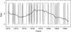 |
Fig. 1 Part of the function sgnA for the asymmetry in sunspot areas. The solid curve shows sgnA smoothed over four years (49 months). |
Variations in x and sgnx for many physically interesting functions display similar correlation properties.
In general, the correlation between the original realization and its sign is 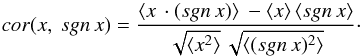 (4)For centered distribution
 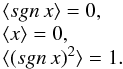 (5)According to the general definition for any functions,
  (6)From Eqs. (4)–(6) we obtain
 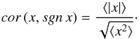 (7)Now, let us find the expression for cor (x, | x |). Similarly to Eq. (4), we have
 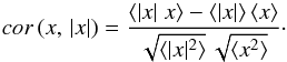 (8)If the distribution is centered, all components in the numerator are equal to zero, while the denominator does not go to zero. If the distribution is not centered, but the function is essentially alternating (the number of pluses and minuses is approximately equal), the components of the numerator are small quantities. Hence,
  (9)Thus, generally we can expect that the correlation coefficient for the functions sgnx and x will be high, and the correlation coefficient for the functions | x | and x will be low.
Let us consider by way of example the monochromatic harmonic function x = x0 cos(ωt). Smoothing over a window much larger than the function period (or over a whole number of periods) will yield  (10)Then, substituting Eq. (10) into Eq. (7), we will obtain
  (11)As another example, let us use for x the standard centered normalized law:
  (12)In this case, we have As a result, using Eq. (7), we obtain
  (13)This means that the sign of the functions most commonly dealt with in physical experiments is highly correlated with the function itself and reflects its basic properties. On the other hand, the correlation of the absolute value with the parent function must not be high.
3. The sign of asymmetry and long-term variations of solar activity
3.1. Some general properties of the north-south asymmetry
Before dwelling on the sign of NS asymmetry we shall briefly describe some of its general properties. This work is based on the analysis of monthly mean total sunspot areas and total number of sunspot groups for the period 1874–2013. Henceforth, these data will be called initial indices. These data up to 1976 were calculated from the Greenwich Catalog and, later, from its continuation compiled by the National Oceanic and Atmospheric Administration and US Air Force1. The databases contain heliographic coordinates and areas of all sunspot groups observed on a given day. Therefore, one should have in mind that our analysis is based on the asymmetry of the sunspot parameters and, therefore, all conclusions relate to the sunspot formation zone.
There are several definitions of the NSA. Most frequently, this quantity is determined as  (14)where N and S are the values of the corresponding activity indices for the northern and southern hemisphere, respectively. This is a so-called “normalized” NSA. We can also mention the “non-normalized” asymmetry (e.g., see Ballester et al. 2005) where NSA is determined as the difference of the corresponding indices. Here, we will use the definition given above in Eq. (14).
The main NSA properties, found in our earlier studies, are described in Badalyan & Obridko (2011) and are briefly listed below.
-
1.
The analysis carried out by various au-thors (e.g., see Newton & Mil-som 1955; Waldmeier 1971; Sýkora 1980; Rušin 1980)made us suggest that the behavior of the NS asymmetry in differ-ent indices of solar activity has common features. This sugges-tion was corroborated in Badalyan et al. (2005)where the asymmetry was studied in four activity indices relevantto different layers in the solar atmosphere: the coronal green-linebrightness at 530.3 nm, the total sunspot area, the total sunspotnumber for 1939–2001, and the integral magnetic flux for 1975–2001. It was shown that the characteristic time variation of theasymmetry value was similar in all activity indices both on largeand on small timescales. The asymmetry has no strict periodicity,and its time variations are not directly related to the 11-yr activ-ity cycle. On the other hand, the asymmetry exhibits periodicvariations with a quasi-period of about 12 yr.
-
2.
The asymmetry of the indices under examination displays quasi-biennial oscillations (QBO), the QBO being much better pronounced in the asymmetry than in the indices themselves. It was found that the long periods of strengthening and weakening of QBO in the asymmetry of these indices occurred synchronously. This effect was discovered on a limited time interval from 1940 to 2001 (Badalyan et al. 2005). In this period, NSA was mainly positive. In our later work (Badalyan & Obridko 2011), we extended the analysis to a longer time interval. The existence of QBO was corroborated over sufficiently long intervals of negative asymmetry at the beginning of the 20th century. At the beginning of the 21st century, we also observed periods of strong negative asymmetry. We should also mention the work by Sýkora & Rybák (2010), who revealed and studied QBO in the north-south asymmetry by using the autocorrelation method.
-
3.
It was interesting to find negative correlation between the QBO intensity and A over long time intervals. To study this phenomenon, we applied Spectral Variation Analysis (SVAN) – expansion of the data under examination into Fourier series in a moving time window (for details see Badalyan & Obridko 2011). The phenomenon is clearly pronounced as a significant decay of QBO in the mid 1960s, which coincides with the period of particularly strong increase of A, and at the beginning of the 20th and 21st centuries when considerable negative asymmetry was observed. The negative correlation between the QBO intensity and the asymmetry value does not depend on the asymmetry sign (see Badalyan & Obridko 2011).
Figure 2 illustrates the third property, that is, the negative correlation between the QBO intensity and the asymmetry value A. Each point on this plot is the value averaged over a 132-months moving window. The solid circles stand for the positive asymmetry (the northern hemisphere dominates) and the open ones, for the negative asymmetry (the southern hemisphere dominates). The left-hand panel shows separate plots for the positive and negative asymmetry (the correlation coefficients are 0.68 and 0.40, respectively). The plot on the right-hand panel represents the asymmetry absolute value (the correlation coefficient is 0.46); the solid and open circles on both panels designate the positive and negative A, respectively. One can see that the QBO intensity reaches its maximum value when the asymmetry goes to zero, that is, when both hemispheres are working in unison. The presence of significant asymmetry (regardless of sign) decreases the intensity of quasi-biennial oscillations. Therefore we can suggest that in the periods of strong asymmetry, such as the Maunder minimum (see Sokoloff 2005; Ribes & Nesme-Ribes 1993; Sokoloff & Nesme-Ribes 1994), quasi-biennial oscillations must be absent.
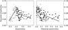 |
Fig. 2 Anticorrelation between the asymmetry value and QBO intensity separately for the positive (solid circles) and negative (open circles) asymmetry (left) and for the asymmetry modulus (right). |
3.2. Basic properties of north-south asymmetry sign
Now we proceed directly to the analysis of the asymmetry sign variations. Juxtaposed in Fig. 3 (left panel) are the curves that represent the smoothed time variations of the asymmetry value A and its sign sgnA (the four-year moving average). As seen from the figure, as should be expected variations have similar features, with the correlation between the curves reaching 0.96.
The periodograms calculated over the entire observation period also coincide (Fig. 3, right panel). The correlation coefficient for the curves on the right panel in the range of the periods from 50 to 250 months is 0.94. On both periodograms, the 11-yr period is weakly pronounced; however, one can clearly identify a quasi-period of 12 yr.
Figure 4 represents spectral variation diagrams (SVD) for the asymmetry A (top) and the asymmetry sign sgnA (bottom) (SVD construction method is described in Badalyan et al. 2005; Badalyan & Obridko 2009, 2011). A 132-month moving window was applied for calculations with a shift of 12 months. The periods represented in Fig. 4 range from six to 40 months. The scale at the bottom shows the oscillation amplitudes. The figure illustrates the similarity of both spectral variation diagrams in the basic details. Amplification of quasi-biennial oscillations (blue) occurs at the same frequencies and is virtually simultaneous. On both SVDs, one can also see the period of amplified quasi-biennial oscillations change gradually from about three years at the end of the 19th century to two years in the late 20th and early 21st century, as noted in Badalyan & Obridko (2011). The comparison of both maps at 702 spatially coinciding points reveals a high correlation (Fig. 5, left panel) with a coefficient of 0.70.
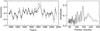 |
Fig. 3 Left – smoothed asymmetry (solid curve) and asymmetry sign (dashed curve); right – periodograms (power spectra) for the asymmetry and its sign. |
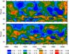 |
Fig. 4 Comparison of Spectral Variation Diagram for the asymmetry A of sunspot areas (top) and the asymmetry sign sgnA (bottom). The periods are given in months. |
The right panel in Fig. 5 represents the time variation of QBO intensity for the asymmetry (solid curve) and its sign (dashed curve). Here, we have summarized the squared amplitudes of the periods from ~15 to ~33 months (the total of six harmonics). Both curves display a similar time behavior. The correlation coefficient is 0.65. In this figure, one can also see oscillations with a period of about 40 yr (see also Badalyan & Obridko 2011).
The comparison shows that, in fact, the sign of the asymmetry is what determines its value on our characteristic smoothing timescales. The smoothed time variation of sgnA is similar to that of the asymmetry value and displays the same properties. The periodogram of the function sgnA mainly coincides with the asymmetry periodogram (Fig. 3, right). We recall that the first basic property of NSA mentioned above suggests the similarity of its time variation in different indices of solar activity. The spectral variation diagram of sgnA, as that of the asymmetry value (Fig. 4), displays periodic amplification of quasi-biennial oscillations. The second property is that quasi-biennial oscillations in the asymmetry are particularly well pronounced. It should be noted here that the third important property of NSA – anticorrelation between the asymmetry value and the intensity of QBO (see Fig. 2) – is not revealed in the asymmetry sign (see Sect. 3.3 below).
3.3. Statistics of sign alternation of the asymmetry
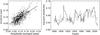 |
Fig. 5 Correlation between the maps shown in Fig. 4 in the range of the periods from six to 40 months (left) and time variation of the squared amplitudes for the asymmetry and its sign in the QBO range (right). |
In general, the time variation of the asymmetry sign is a sequence of the intervals when the asymmetry is positive or negative. The length of these intervals varies significantly. At the end of each interval, the asymmetry function “switches over” from one sign to the other. It is particularly interesting to analyze the statistics of these intervals. The question is whether there is a regularity in their distribution. The interest in this question is stimulated by the fact that the period of low activity in the 17th century (Maunder minimum) coincided with a long interval when the activity was mainly observed in the southern hemisphere (negative asymmetry) (see Sokoloff 2005; Ribes & Nesme-Ribes 1993; Sokoloff & Nesme-Ribes 1994; Nagovitsyn et al. 2004).
By analogy with the term accepted in geomagnetism, the intervals when the asymmetry has one sign can be called “monochrome” intervals. This term seems natural when analyzing the time diagrams on which the intervals of one or other polarity are painted black or white, respectively. On such diagrams, one can consider either the intervals of positive and negative asymmetry separately or the distribution of all monochrome intervals regardless of the sign.
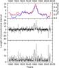 |
Fig. 6 Top – the asymmetry with sign (blue curve) and the lengths of monochrome intervals (red curve) smoothed over 132-month moving window; middle and bottom – the lengths of monochrome intervals with and without regard for the sign, respectively. |
The upper panel in Fig. 6 illustrates the time dependence of the asymmetry with sign smoothed over 132-month window, that is, about one cycle (blue curve) and the lengths of the monochrome intervals smoothed in the same way (red curve). The lengths of the monochrome intervals versus time with and without regard for the sign are represented on the middle and lower panels, respectively. The graph on the middle panel is plotted as follows. The time of change of the asymmetry sign is defined and, then, all points until the next sign inversion are assigned the value equal to the length of this monochrome interval and the sign corresponding to the asymmetry sign in this interval. For example, if the length of the monochrome interval is + 7 or −7 depending on the asymmetry sign, all points inside the interval are assigned the value + 7 or −7. The graph on the lower panel is plotted in the same way, but the asymmetry sign inside the monochrome intervals is neglected. As seen from Fig. 6, the smoothed curve of the lengths of the monochrome intervals resembles very much the smoothed asymmetry curve.
We now consider the distribution of the monochrome intervals with and without regard for the sign. We designate the distribution histograms for all monochrome intervals, positive intervals (northern hemisphere dominates), and negative intervals as n (L), n (Lp), and n (Lm), respectively. Each histogram is normalized to the total number of the monochrome intervals ∑ n (L). This will yield the occurrence rate of all monochrome intervals ϕ(L), positive intervals ϕ(Lp), and negative intervals ϕ(Lm). These distributions are illustrated in Fig. 7. The histograms shown in Fig. 7 can be approximated by exponential law of the form:  (15)One can see that ϕ (Lp) and ϕ (Lm) virtually coincide statistically, while ϕ (L) is approximately twice as high (for approximation parameters see Table 1).
Exponential approximation parameters.
The length of the monochrome intervals in Fig. 6 can be regarded as the “weight” of the sign: the longer the monochrome interval, the larger the weight of its sign + 1 or −1 in the smoothed curve. If we plot the SVD for the lengths of the monochrome intervals with their signs (the series in Fig. 6, middle panel), we shall see that it resembles very much the SVD for the asymmetry sign (Fig. 4, lower panel); the correlation of the corresponding maps is 0.68. It is interesting to note here that anticorrelation between the QBO intensity and the asymmetry value, which is not revealed in the asymmetry sign (see Fig. 2), is seen in the lengths of the monochrome intervals nearly as well as in the asymmetry (the third basic property of the asymmetry).
Of course, it is assumed that the occurrence rate functions within each smoothing window do not differ much from the functions ϕ(L), ϕ(Lp), and ϕ(Lm), obtained for the entire interval under consideration. This assumption is sufficiently correct since we are using quite a large smoothing window of 132 months. Of course, some deviations are possible, especially as concerns the occurrence rate of very long monochrome intervals. However, such intervals are very few and do not affect the resulting smoothed curve significantly (blue curve in Fig. 6). They manifest themselves in deviation from the standard Poisson distribution.
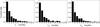 |
Fig. 7 Histograms of the occurrence rates of monochrome intervals of different lengths: all intervals (left), positive intervals (northern hemisphere dominates, middle), and negative intervals (southern hemisphere dominates, right). |
Thus, for monochrome intervals from one to 12 months long, the histogram corresponds to the equation: 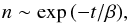 (16)with a characteristic time interval of the constant asymmetry sign β = 1.724 months.
This means that the distribution of the monochrome intervals obeys the statistical law of independent events for the interval lengths up to a year. This conclusion seems to be very important to the up-to-date dynamo models. Pipin & Sokoloff (2011), Pipin et al. (2012), Sokoloff et al. (2010, 2012) arrived at the same conclusion concerning different amplitudes of solar cycles (such as the Maunder minimum). In particular, a simple, finite-dimensional geodynamo model was proposed by the aforementioned authors, which is based on the mean-field electrodynamics and reproduces the inversions of the geomagnetic field. In this model, the inversion scale is rather close to that really observed. There is no need to change the hydrodynamic parameters of the problem essentially to obtain inversions in terms of such a model. It is sufficient just to take into account the fluctuations of the α-effect. The existence of abnormal cycles is explained by a random fluctuation of parameter α in the traditional Parker dynamo.
Variations in the asymmetry sign on small timescales may be due to random fluctuations in the Babcock-Leighton mechanism. In particular, Goel & Choudhuri (2009) have shown that, as a result of such fluctuations, the poloidal field in one hemisphere becomes stronger than in the other. This methodology is similar to that applied in Dikpati et al. (2006) and, as a matter of fact, it can be used for prognostic purposes.
There is a nonzero number of the intervals longer than a year. For example, if we integrate the obtained approximation equation from 12 months to infinity, we will obtain the value 0.95. Hence, not more than one monochrome interval longer than a year could be observed during the observation period from 1874 to 2013, while actually there were 11 (see Fig. 6, lower panel).
Dikpati et al. (2007) calculated the amplitude of cycles separately for each hemisphere using the prognostic scheme proposed earlier in (Dikpati et al. 2006). The calculation parameters were the same as used in calculating the cycle amplitude without separation of hemispheres. It turned out that the scheme describes the amplitude of cycles quite satisfactorily (see Figs. 9, 10, and 12 therein). However, it works well when the smoothing is performed over not less than 13 rotations. Variations in the asymmetry sign over shorter intervals cannot be described by this scheme.
On the other hand, Chatterjee & Choudhuri (2006) associated the long-lasting differences in the amplitude of cycles with fluctuations in the Babcock-Leighton model of flux transfer. Minor (less than 1%) differences in the amplitude of the meridional flux in the hemispheres lead to significant changes in the amplitude and relative phase of the cycles in the northern and southern hemispheres.
Cox (1968) suggested that inversion of the geomagnetic field is a Poisson process, and the length of the intervals of constant polarity (monochrome intervals) is determined by P(t) ∝ exp(−t/T). This is more or less true for the intervals <500 thousand years. However, one can also see a “heavy tail” of long intervals.
It is hard to say how randomly long monochrome intervals appear. We can note that the number of long positive monochrome intervals increases in the period of high activity cycles. On the other hand, there is no reason to reject the hypothesis of random occurrence of long positive monochrome intervals.
We note that the number of switchover points does not depend on the phase of the cycle. This is true both for all points and, separately, for the starting points of long and short monochrome intervals.
4. Properties of the asymmetry modulus
4.1. Asymmetry modulus and its relation to the level of solar activity
We consider now the absolute value of the NSA. Its behavior differs drastically from that of the asymmetry itself. This is shown in Fig. 8, which represents part of the series of asymmetry in sunspot areas for the period 1920–2000. The asymmetry absolute values display a strict 11-yr periodicity, which is corroborated by the smoothed Wolf numbers (Version 1.0) shown at the bottom of Fig. 8.
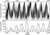 |
Fig. 8 Absolute value of the asymmetry of the total sunspot areas (top) and the annual mean Wolf numbers (bottom). The cycle numbers are indicated. |
The time dependence of the absolute value of asymmetry (“absolute asymmetry”) in sunspot numbers and areas for the entire period 1874–2013 is illustrated in Fig. 9. The figure provides the four-year moving means. One can clearly see that both curves are similar; however, the curve of absolute asymmetry for the total sunspot area (solid curve) goes noticeably higher than that for the total sunspot number. This suggests that, despite the close similarity of the behavior of the normalized asymmetry in different activity indices (see Fig. 3 in Badalyan & Obridko 2011), which demonstrates the normalized asymmetry smoothed by a four-year window, the asymmetry moduli per se are different. At first sight, the corresponding curves in the above-mentioned figure nearly coincide, differing only by a factor of 0.9. The cause of this discrepancy is not quite clear. We can suggest that this is the result of a nonlinear relation between different activity indices, in particular, the relation between the number of sunspots and their total area. In other words, the points characterizing the latter in each given cycle do not represent regular dependence with a spread, but rather form a closed curve of the type of hysteresis loop (see Fig. 1 in Badalyan & Obridko 2011).
Thus, the analysis of the absolute asymmetry without sign reveals some new properties of the asymmetry, which are not seen if the sign is taken into account. The most interesting fact is that the peaks of the absolute asymmetry fall on the cycle minima.
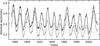 |
Fig. 9 Smoothed absolute asymmetry for sunspot areas (solid curve) and for total sunspot numbers (dotted curve). |
According to the definition of the asymmetry Eq. (14), the numerator N−S and the denominator N + S become very small in the vicinity of the cycle minimum, which leads to the uncertainty of the type 0:0. Therefore, even casual relative fluctuations of the initial indices in the northern and southern hemispheres may result in the increase or decrease of the absolute asymmetry A. If the numerator in Eq. (14) goes to zero slower than the denominator, a maximum appears on the curve in Fig. 9.
Thus, it may be suggested that imbalance between the hemispheres (the measure of which is the NSA) changes during a cycle. In order to corroborate this suggestion, we have analyzed variations in the difference and sum of the initial parameters in different phases of the activity cycle. The results are illustrated in Fig. 10. The upper panel represents the denominator N + S. The red curve is the four-year (49 months) moving average. The middle panel shows N + S divided by the moving average ⟨ N + S ⟩ (black curve). We call this the “moving normalization”. The red curve on this panel is the subsequent four-year averaging. We call this curve the “averaged moving normalization”. Similar calculations were performed for the absolute value of the numerator | N−S |. The final results are represented in Fig. 10 (lower panel). The red curve here is identical with the red curve on the middle panel. The blue curve shows the normalized moving average for | N−S |.
The lower panel in Fig. 10 shows that in the epochs of solar maximum, the curves | N−S | and N + S coincide. This means that both hemispheres function virtually in a single regime. At the cycle minima, however, one can see a noticeable difference: the curve for | N−S | (blue) goes much higher than the curve for N + S.
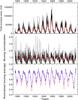 |
Fig. 10 Top – N + S for total sunspot areas, the red curve represents four-year (49 months) moving average. Middle – N + S divided by ⟨ N + S ⟩ (moving normalization), the red curve is subsequent four-year moving average. Bottom – the red curve represents N + S (the same as on the middle panel), the blue curve shows the normalized moving average for | N−S |. |
To obtain the final result, we use the method of superposition of epochs taking into account the cycle phase. In this work, the phase of the cycle was determined in accordance with Mitchell (1929) as 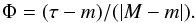 (17)Here, τ is the current time, and M and m are, respectively, the times of the nearest 11-yr maximum and minimum. Thus, according to Eq. (17), the phase is 0 at the minimum of each activity cycle, −1 at the maximum of the previous cycle, and + 1 at the maximum of the following cycle. The phase is positive at the ascending branch of the cycle and negative at its descending branch. Plotting the data for several cycles versus the cycle phase is equivalent to applying the method of superposition of epochs. In doing so, we naturally assume that the evolution of activity in all cycles follows a single scenario (e.g., see Vitinskii et al. 1986; Kuklin et al. 1989).
We calculated the moving mean normalized values versus the cycle phase from −1.0 to + 1.0 with a 0.04 step. Figure 11 (left) illustrates N + S (lower curve) and | N−S | (upper curve). The curve on the right panel shows the ratio of these quantities during a cycle, that is, a kind of mean cycle for the absolute asymmetry. Thus, we obtain that the moving mean normalized values for | N−S | are much higher at the minimum of the cycle than at its maximum (see Fig. 10), and, therefore, the NSA derived from these values is maximal at the minimum of the cycle.
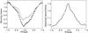 |
Fig. 11 Left – the moving mean normalized values for | N−S | (upper curve, open circles) and N + S (lower curve, solid circles) versus the phase of the activity cycle; right – the ratio of these curves (mean cycle for the absolute asymmetry). |
4.2. Prognostic value of the asymmetry modulus
Let us shift the series of absolute asymmetry in sunspot areas (see Fig. 9) forward by half a cycle, that is, by 5.5 yr, and impose it on the smoothed Wolf number series. Both series are smoothed by a four-year window. The result of the superposition is shown in Fig. 12. Despite a similar time behavior of both series, one can clearly see that the amplitudes of their minima and maxima are different. During a long period of relatively low cycles at the end of the 19th century and in the first third of the 20th century, the absolute asymmetry displays high maxima. Then, before cycles 18 and 19, the asymmetry maxima decreased significantly, while the Wolf number maxima in the corresponding cycles (1947 and 1958) increased. Later, the relatively high asymmetry values at the minima of the subsequent cycles correspond to a gradual decline of activity in the second half of the 20th century. So, we can conclude that the higher the asymmetry value at the cycle minimum, the lower the amplitude of maximum of the following cycle.
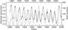 |
Fig. 12 Absolute asymmetry for sunspot areas shifted forward by half a cycle (solid curve) and the Wolf numbers (dotted curve). The lower timescale refers to the Wolf numbers; the upper timescale shifted by half a cycle refers to the absolute asymmetry. |
This relationship can be examined in more detail on the correlation diagram. The negative correlation between the asymmetry modulus at the cycle minimum and the amplitude of the following activity maximum is 0.777 (Fig. 13, left). The same figure (center) shows a scatter plot of the relationship between the asymmetry modulus and the Wolf numbers at the minima of the same cycles. Here, again, we can see a noticeable negative correlation with a coefficient equal to 0.658.
This suggests that the increasing asymmetry modulus (i.e., the increasing imbalance between the hemispheres) at the cycle minimum will decrease the sunspot production rate both at the minimum of the given cycle and at the maximum of the following one (i.e., will decrease their amplitude). This effect apparently lies at the heart of the well-known method of forecasting the amplitude of the cycle from the preceding Wolf number minimum. Thus, Hathaway et al. (1999) obtained the correlation between the Wolf numbers at the cycle minimum and the amplitude of the following maximum for cycles 1–22 equal to 0.723. Our correlation coefficient for cycles 12–24 is 0.837 (Fig. 13, right).
Therefore, the relations obtained in our work can be used for predicting the next cycle of solar activity along with many other methods (e.g., see Jiang et al. 2015; Wang & Sheeley 2009). For a complete review of the existing forecasts of cycle 24 see Pesnell (2008).
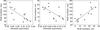 |
Fig. 13 Left – correlation between the asymmetry modulus at the cycle minimum and the amplitude of the following cycle; center – correlation between the asymmetry modulus and the Wolf numbers at the minimum of the cycle; right – correlation between the Wolf numbers minimum and the following maximum. |
Thus, the absolute value of the asymmetry has some specific statistical properties associated apparently with processes responsible for the amplitude of the activity cycle. This is evident, in particular, from the prognostic value of the asymmetry modulus identified here.
5. Main conclusions and discussion
The north-south asymmetry of solar activity is the characteristic and measure of the imbalance between the two solar hemispheres. As the frequency and amplitude characteristics of this phenomenon can be determined by different mechanisms, we analyzed the NSA as a superposition of two realizations: the asymmetry sign (signature sgnA) and the asymmetry absolute value (modulus | A |). These two parameters are considered separately, and it is shown that each of them plays a specific, important role.
It is the asymmetry sign that provides basic information on the asymmetry time behavior, including its ~12-yr periodicity and the presence of quasi-biennial oscillations. The sign determines the value of the asymmetry on typical timescales. The smoothed time variation of sgnA is similar to that of the asymmetry value and displays the same particularities. The periodogram of the sgnA function virtually coincides with the asymmetry periodogram. The spectral-time analysis of the asymmetry and sgnA reveals a periodic enhancement of quasi-biennial oscillations. The asymmetry sign does not demonstrate anti-correlation between the asymmetry value and QBO intensity over long time intervals (as seen in Fig. 2). However, the anti-correlation is still observed if instead of the asymmetry sign series, we use the lengths of a series of one-sign (“monochrome”) intervals characterizing the weight of the asymmetry sign.
A fundamental finding of this analysis is the fact that the distribution of “monochromatic” intervals (intervals of the asymmetry of one sign) obeys the Poisson distribution, that is, corresponds to the statistics of random processes. Random processes in the sunspot formation region are now extensively used in many dynamo models (Kitchatinov & Olemskoy 2016; Pipin et al. 2014). Characteristic times of the order of two months are consistent with those used in these models.
The asymmetry modulus has quite different statistical meaning, because it characterizes the degree of domination of one or the other hemisphere without specifying which of the hemispheres is dominant. The behavior of the NSA modulus differs drastically from that of the asymmetry with sign. It is characterized by a strict 11-yr periodicity similar to the Wolf number cycle shifted by half a cycle; that is, the maximum of the asymmetry modulus coincides with the sunspot minimum. It is shown that the obtained increase in the asymmetry modulus at the minimum of the cycle is not the mere result of division by a small quantity in Eq. (14) when determining A. In fact, the difference of the activity indices in the two hemispheres at the cycle minimum tends to zero more slowly than their sum, which is why the absolute asymmetry is maximum in this epoch (see Fig. 11).
We have revealed negative correlation between the asymmetry modulus at the cycle minimum and the amplitude of the upcoming solar cycle. It is shown that the imbalance between the hemispheres at the minimum of the cycle is stronger than in the other phases.
Thus, the asymmetry modulus has a prognostic meaning: the larger the asymmetry modulus at the cycle minimum, the lower the following cycle. The physical significance of this conclusion is very important. It is in the epoch of sunspot minimum that the global field of the following cycle is formed, from which, subsequently, the mechanism of Ω-dynamo generates local fields. The increasing asymmetry at the cycle minimum apparently affects the generation of the following cycle. This may be due to the fact that with respect to the Ω-dynamo the initial poloidal structure is a dipole field, which is, in principle, anti-symmetric in sign and symmetric in value relative to the equator. The differential rotation transforms the poloidal structure into toroidal fields. It should be noted here that differential rotation, being a relatively independent process, is not necessarily symmetric about the equator.
Certain differences in the characteristics of differential rotation in the northern and southern hemispheres have been reported by many authors (e.g., see Badalyan & Sýkora 2006; Zhang et al. 2011; Rightmire-Upton et al. 2012; Li et al. 2013). Anyway, the theory does not forbid the violation of differential rotation. So, the arising toroidal field is, by definition, symmetric about the rotation axis, anti-symmetric about the equator in sign, and, strictly speaking, it may have no symmetry at all about the equator in absolute value. Later on, the α-effect converts this not entirely symmetric toroidal field into the new symmetric poloidal field. We note again that since the parameter α is rather small, the fluctuations may reach 20 percent of the mean value (Sokoloff et al. 2012, 2010; Pipin et al. 2012). Thus, the dependence of the α-effect on possible fluctuations and characteristics of the asymmetry may be rather strong. The violation of synchronism in the work of the hemispheres must affect the generation of the poloidal field. Thus, the asymmetry is not only the measure of imbalance of the hemispheres, but, to a certain extent, an indication of the reduced efficiency of generation of the magnetic field of the following cycle.
It is interesting to note that a long-lasting (about 70 yr) imbalance between the hemispheres was observed during the Maunder minimum (Sokoloff 2005; Sokoloff & Nesme-Ribes 1994; Ribes & Nesme-Ribes 1993). In fact, only the southern hemisphere was active in that period. Constant prevalence of activity in the southern hemisphere manifested itself in very high values of the asymmetry amplitude. This is consistent with the above-mentioned negative correlation between the asymmetry amplitude and the level of sunspot activity.
It also follows from Fig. 2 that with the increase of the asymmetry amplitude, the QBO intensity decreases. Therefore, we may suggest that both the amplitude of the 11-yr cycle and the QBO intensity must decrease in the periods when the asymmetry amplitude (regardless of its sign) remains high for a long time.
Thus, there are quite a lot of factors that can lead to NS asymmetry of the solar magnetic field. There is no need to change significantly the main scheme of the magnetic field generation. NSA can be caused by the asymmetry in the occurrence of various processes that form part of the dynamo mechanisms. In particular, this can be the asymmetry in the meridional circulation rate (see Cameron & Schüssler 2012; Belucz & Dikpati 2013; Shetye et al. 2015) or in the α-effect (see Belucz et al. 2013), the diffusion through the equator at large depths or in the surface layer (Norton et al. 2014), or various stochastic effects in the Babcock-Leighton model (Goel & Choudhuri 2009; Dikpati et al. 2007, 2006; Hoyng et al. 1994; Olemskoy & Kitchatinov 2013; Olemskoy et al. 2013). With an appropriate choice of parameters, one will be able to explain both the synchronization of cycles in the two hemispheres and their divergence by up to two years in phase and up to 40 percent in amplitude (Norton et al. 2014). However, the question of the origin of small fluctuations in the sign of asymmetry remains open. What exactly causes the asymmetry of the components of the generation mechanism is not clear, and we hope that the present study may shed some light on this issue.
Our work has shown that the asymmetry sign determines the general pattern of the asymmetry time variation. We believe that this conclusion has a deep philosophical meaning and, apparently, reflects the general law of dualistic logic. The description of the result of a research project begins with a statement like “yes-no”. This is usually enough to get an initial idea of the research object. In fact, relying solely on the pluses and minuses, one can easily identify the general features of an object, process, or phenomenon. For example, the neutral lines drawn on a magnetic map yield a fairly good idea of the relationship between different parameters and processes (Makarov & Sivaraman 1983; Makarov et al. 1983).
It is enough to specify the zeroes of a function and we will get an idea of its properties, however, going to the heart of the problem requires additional details.
In this context, it can be assumed that the asymmetry sign (i.e., the indicator of predominance of a particular solar hemisphere) is actually the asymmetry. It is the sign of the asymmetry that provides us with basic information on its properties, while the asymmetry modulus reveals quite different statistical features associated with a standard 11-yr periodicity.
Acknowledgments
The work was supported by the Russian Foundation for Basic Research, Project No. 14-02-00308.
References
- Badalyan, O. G. 2011, Astron. Zh., 88, 1008 [NASA ADS] [Google Scholar]
- (English translation 2011, Astron. Rep., 55, 928) [NASA ADS] [CrossRef] [Google Scholar]
- Badalyan, O. G., & Obridko, V. N., 2009, in Astronomical Year: Solar and Solar-Terrestrial Physics, ed. A. V. Stepanov, St.-Petersburg, Astron. Obs. RAS at Pulkovo, 37 [in Russian] [Google Scholar]
- Badalyan, O. G., & Obridko, V. N. 2011, New Astron., 16, 357 [NASA ADS] [CrossRef] [Google Scholar]
- Badalyan, O. G., & Sýkora, J. 2006, Adv. Space Res., 38, 906 [NASA ADS] [CrossRef] [Google Scholar]
- Badalyan, O. G., Obridko, V. N., Rybák, J., & Sýkora, J. 2005, Astron. Zh., 82, 740 (English translation 2005, Astron. Rep., 49, 659) [Google Scholar]
- Badalyan, O. G., Obridko, V. N., & Sýkora, J. 2008, Sol. Phys., 247, 379 [NASA ADS] [CrossRef] [Google Scholar]
- Ballester, J. L., Oliver, R., & Carbonell, M. 2005, A&A, 431, L5 [NASA ADS] [CrossRef] [EDP Sciences] [Google Scholar]
- Belucz, B., & Dikpati, M. 2013, ApJ, 779, 9 [Google Scholar]
- Belucz, B., Forgács-Dajka, E., & Dikpati, M. 2013, Astron. Nachr., 334, 960 [NASA ADS] [CrossRef] [Google Scholar]
- Boyer, D. W., & Levy, E. H. 1984, ApJ, 277, 848 [NASA ADS] [CrossRef] [Google Scholar]
- Cameron, R. H., & Schüssler, M. 2012, A&A, 548, A57 [NASA ADS] [CrossRef] [EDP Sciences] [Google Scholar]
- Carbonell, M., Oliver, R., & Ballester, J. L. 1993, A&A, 274, 497 [NASA ADS] [Google Scholar]
- Carbonell, M., Terradas, J., Oliver, R., & Ballester, J. L. 2007, A&A, 476, 951 [NASA ADS] [CrossRef] [EDP Sciences] [Google Scholar]
- Chatterjee, P., & Choudhuri, A. R. 2006, Sol. Phys., 239, 29 [NASA ADS] [CrossRef] [Google Scholar]
- Cox, A. V. 1968, J. Geophys. Res., 73, 3247 [NASA ADS] [CrossRef] [Google Scholar]
- Dikpati, M., de Toma, G., & Gilman, P. D. 2006, Geophys. Res. Lett., 33, L05102 [NASA ADS] [CrossRef] [Google Scholar]
- Dikpati, M., Gilman, P. A., de Toma, G., & Ghosh, S. S. 2007, Sol. Phys., 245, 1 [NASA ADS] [CrossRef] [Google Scholar]
- Goel, A., & Choudhuri, A. R. 2009, Res. Astron. Astrophys., 9, 115 [NASA ADS] [CrossRef] [Google Scholar]
- Jiang, J., Cameron, R. H., & Schüssler, M. 2015, ApJ, 808, L6 [NASA ADS] [CrossRef] [Google Scholar]
- Hathaway, D. H., & Wilson, R. M. 1990, ApJ, 357, 271 [NASA ADS] [CrossRef] [Google Scholar]
- Hathaway, D. H., Wilson, R. M., & Reichmann, E. J. 1999, J. Geophys. Res., 104, 22375 [NASA ADS] [CrossRef] [Google Scholar]
- Hoyng, P., Schmitt, D., & Teuben, L. J. W. 1994, A&A, 289, 265 [NASA ADS] [Google Scholar]
- Kambry, M. A., & Nishikawa, J. 1990, Sol. Phys., 126, 89 [NASA ADS] [CrossRef] [Google Scholar]
- Kitchatinov, L. L., & Olemskoy, S. V. 2016, MNRAS, 459, 4353 [Google Scholar]
- Knaack, R., Stenflo, J. O., & Berdyugina, S. V. 2004, A&A, 418, L17 [NASA ADS] [CrossRef] [EDP Sciences] [Google Scholar]
- Kuklin, G., Obridko, V. N., & Vitinsky, Yu. 1989, Solar Terrestrial Predictions Proc., Leura, Australia, 1, 474 [Google Scholar]
- Li, K. J., Wang, J. X., Xiong, S. Y., et al. 2002, A&A, 383, 648 [NASA ADS] [CrossRef] [EDP Sciences] [Google Scholar]
- Li, K. J., Shi, X. J., Xie, J. L., et al. 2013, MNRAS, 433, 521 [NASA ADS] [CrossRef] [Google Scholar]
- Makarov, V. I., & Sivaraman, K. R. 1983, Sol. Phys., 85, 227 [NASA ADS] [CrossRef] [Google Scholar]
- Makarov, V. I., Fatianov, M. P., & Sivaraman, K. R. 1983, Sol. Phys., 85, 215 [NASA ADS] [CrossRef] [Google Scholar]
- Mariş, J., Popescu, M. D., & Mierla, M. 2002, Rom. Astron. J., 12, 131 [Google Scholar]
- Mitchell, S. A. 1929, Handb. Astrophys., 4, 231 [NASA ADS] [Google Scholar]
- Mordvinov, A. V. 2007, Sol. Phys., 246, 445 [NASA ADS] [CrossRef] [Google Scholar]
- Nagovitsyn, Yu. A. 1998, Izvestiya Glav. Astron. Obs., 212, 145 [in Russian] [Google Scholar]
- Nagovitsyn, Yu. A., Ivanov, V. G., Miletsky, E. V., & Volobuev, D. M. 2004, Sol. Phys., 224, 103 [NASA ADS] [CrossRef] [Google Scholar]
- Newton, H. W., & Milsom, A. S. 1955, MNRAS, 115, 398 [NASA ADS] [CrossRef] [Google Scholar]
- Norton, A. A., Charbonneau, P., & Passos, D. 2014, Space Sci. Rev., 186, 251 [NASA ADS] [CrossRef] [Google Scholar]
- Obridko, V. N., & Shelting, B. D. 2000a, Astron. Zh., 77, 124 (English translation 2000, Astron. Rep. 44, 103) [Google Scholar]
- Obridko, V. N., & Shelting, B. D., 2000b, Astron. Zh., 77, 303 (English translation 2000, Astron. Rep. 44, 262) [Google Scholar]
- Obridko, V. N., & Shelting, B. D. 2016, Pis’ma Astron. Zh., 42, 694 [Google Scholar]
- (English translation 2016, Astron. Lett., 42, 631) [NASA ADS] [CrossRef] [Google Scholar]
- Olemskoy, S. V., & Kitchatinov, L. L. 2013, ApJ, 777, 8 [Google Scholar]
- Olemskoy, S. V., Choudhuri, A. R., & Kitchatinov, L. L. 2013, Astron. Zh., 90, 501 [Google Scholar]
- (English translation 2013, Astron. Rep., 57, 458) [NASA ADS] [CrossRef] [Google Scholar]
- Pesnell, W. D. 2008, Sol. Phys., 252, 209 [NASA ADS] [CrossRef] [Google Scholar]
- Pipin, V. V., & Sokoloff, D. D. 2011, Phys. Scr., 84, 065903 [NASA ADS] [CrossRef] [Google Scholar]
- Pipin, V. V., Sokoloff, D. D., & Usoskin, I G. 2012, A&A, 542, A11 [NASA ADS] [CrossRef] [EDP Sciences] [Google Scholar]
- Pipin, V. V., Moss, D., Sokoloff, D. D., & Hoeksema, J. T. 2014, A&A, 567, A8 [NASA ADS] [CrossRef] [EDP Sciences] [Google Scholar]
- Ribes, J. C., & Nesme-Ribes, E. 1993, A&A, 276, 549 [NASA ADS] [Google Scholar]
- Rightmire-Upton, L., Hathaway, D. H., & Kosak, K. 2012, ApJ, 761, L4 [NASA ADS] [CrossRef] [Google Scholar]
- Rušin, V. 1980, Bull. Astr. Inst. Czechosl., 31, 9 [NASA ADS] [Google Scholar]
- Shetye, J., Tripathi, D., & Dikpati, M. 2015, ApJ, 799, 11 [Google Scholar]
- Sokoloff, D. D. 2005, Sol. Phys., 224, 145 [NASA ADS] [CrossRef] [Google Scholar]
- Sokoloff, D., & Nesme-Ribes, E. 1994, A&A, 288, 293 [NASA ADS] [Google Scholar]
- Sokoloff, D., Arlt, R., Moss, D., Saar, S. H., & Usoskin, I. 2010, in Solar and Stellar Variability: Impact on Earth and Planets, Proc. IAU Symp., 264, 111 [Google Scholar]
- Sokoloff, D. D., Sobko, G. S., Trukhin, V. I., & Zadkov, V. N. 2012, in Comparative Magnetic Minima: Characterizing quiet times in the Sun and Stars, Proc. IAU Symp., 286, 360 [NASA ADS] [Google Scholar]
- Sýkora, J. 1980, in Solar and Interplanetary Dynamics, eds. M. Dryer, & E. Tandberg-Hanssen, Proc. IAU Symp., 91, 87 [Google Scholar]
- Sýkora, J., & Rybák, J. 2010, Sol. Phys., 261, 321 [NASA ADS] [CrossRef] [Google Scholar]
- Temmer, M., Rybák, J., Bendik, P., et al. 2006, A&A, 447, 735 [NASA ADS] [CrossRef] [EDP Sciences] [Google Scholar]
- Tobias, S. 1997, A&A, 322, 1007 [NASA ADS] [Google Scholar]
- Vitinskii, Yu. I., Kopecký, M., & Kuklin, G. V. 1986, Statistics of Spot-Formation Activity of the Sun (Moscow: Nauka) [in Russian] [Google Scholar]
- Vizoso, G., & Ballester, J. L. 1990, A&A, 229, 540 [NASA ADS] [Google Scholar]
- Waldmeier, M. 1971, Sol. Phys., 29, 332 [NASA ADS] [CrossRef] [Google Scholar]
- Wang, Y.-M., & Sheeley, N. R. Jr. 2009, ApJ, 694, L11 [NASA ADS] [CrossRef] [Google Scholar]
- Weiss, N. 2010, Astron. Geophys., 51, 3.09 [CrossRef] [Google Scholar]
- Zhang, L., Mursula, K., Usoskin, I., Wang, H., & Du, Z. 2011, in First Asia-Pacific Solar Physics Meeting, eds. A. R. Choudhuri, & D. Banerjee, ASI Conf. Ser., 2, 175 [Google Scholar]
- Zolotova, N. V., & Ponyavin, D. I. 2006, A&A, 449, L1 [NASA ADS] [CrossRef] [EDP Sciences] [Google Scholar]
- Zolotova, N. V., & Ponyavin, D. I. 2007, A&A, 470, L17 [NASA ADS] [CrossRef] [EDP Sciences] [Google Scholar]
All Tables
All Figures
|
Fig. 1 Part of the function sgnA for the asymmetry in sunspot areas. The solid curve shows sgnA smoothed over four years (49 months). |
| In the text | |
|
Fig. 2 Anticorrelation between the asymmetry value and QBO intensity separately for the positive (solid circles) and negative (open circles) asymmetry (left) and for the asymmetry modulus (right). |
| In the text | |
|
Fig. 3 Left – smoothed asymmetry (solid curve) and asymmetry sign (dashed curve); right – periodograms (power spectra) for the asymmetry and its sign. |
| In the text | |
|
Fig. 4 Comparison of Spectral Variation Diagram for the asymmetry A of sunspot areas (top) and the asymmetry sign sgnA (bottom). The periods are given in months. |
| In the text | |
|
Fig. 5 Correlation between the maps shown in Fig. 4 in the range of the periods from six to 40 months (left) and time variation of the squared amplitudes for the asymmetry and its sign in the QBO range (right). |
| In the text | |
|
Fig. 6 Top – the asymmetry with sign (blue curve) and the lengths of monochrome intervals (red curve) smoothed over 132-month moving window; middle and bottom – the lengths of monochrome intervals with and without regard for the sign, respectively. |
| In the text | |
|
Fig. 7 Histograms of the occurrence rates of monochrome intervals of different lengths: all intervals (left), positive intervals (northern hemisphere dominates, middle), and negative intervals (southern hemisphere dominates, right). |
| In the text | |
|
Fig. 8 Absolute value of the asymmetry of the total sunspot areas (top) and the annual mean Wolf numbers (bottom). The cycle numbers are indicated. |
| In the text | |
|
Fig. 9 Smoothed absolute asymmetry for sunspot areas (solid curve) and for total sunspot numbers (dotted curve). |
| In the text | |
|
Fig. 10 Top – N + S for total sunspot areas, the red curve represents four-year (49 months) moving average. Middle – N + S divided by ⟨ N + S ⟩ (moving normalization), the red curve is subsequent four-year moving average. Bottom – the red curve represents N + S (the same as on the middle panel), the blue curve shows the normalized moving average for | N−S |. |
| In the text | |
|
Fig. 11 Left – the moving mean normalized values for | N−S | (upper curve, open circles) and N + S (lower curve, solid circles) versus the phase of the activity cycle; right – the ratio of these curves (mean cycle for the absolute asymmetry). |
| In the text | |
|
Fig. 12 Absolute asymmetry for sunspot areas shifted forward by half a cycle (solid curve) and the Wolf numbers (dotted curve). The lower timescale refers to the Wolf numbers; the upper timescale shifted by half a cycle refers to the absolute asymmetry. |
| In the text | |
|
Fig. 13 Left – correlation between the asymmetry modulus at the cycle minimum and the amplitude of the following cycle; center – correlation between the asymmetry modulus and the Wolf numbers at the minimum of the cycle; right – correlation between the Wolf numbers minimum and the following maximum. |
| In the text | |
Current usage metrics show cumulative count of Article Views (full-text article views including HTML views, PDF and ePub downloads, according to the available data) and Abstracts Views on Vision4Press platform.
Data correspond to usage on the plateform after 2015. The current usage metrics is available 48-96 hours after online publication and is updated daily on week days.
Initial download of the metrics may take a while.