| Issue |
A&A
Volume 602, June 2017
|
|
|---|---|---|
| Article Number | A110 | |
| Number of page(s) | 9 | |
| Section | Numerical methods and codes | |
| DOI | https://doi.org/10.1051/0004-6361/201629957 | |
| Published online | 22 June 2017 | |
Gaia eclipsing binary and multiple systems. A study of detectability and classification of eclipsing binaries with Gaia
1 University of Ljubljana, Deptartment of Physics, Jadranska 19, 1000 Ljubljana, Slovenia
e-mail: This email address is being protected from spambots. You need JavaScript enabled to view it.
2 University of Geneva, Department of Astronomy, Chemin des Maillettes 51, 1290 Versoix, Switzerland
3 Villanova University, Department of Astrophysics and Planetary Science, 800 Lancaster Ave, Villanova, PA 19085, USA
4 University of Geneva, Department of Astronomy, Chemin d’Ecogia 16, 1290 Versoix, Switzerland
Received: 25 October 2016
Accepted: 26 March 2017
Abstract
Context. In the new era of large-scale astronomical surveys, automated methods of analysis and classification of bulk data are a fundamental tool for fast and efficient production of deliverables. This becomes ever more important as we enter the Gaia era.
Aims. We investigate the potential detectability of eclipsing binaries with Gaia using a data set of all Kepler eclipsing binaries sampled with Gaia cadence and folded with the Kepler period. The performance of fitting methods is evaluated in comparison to real Kepler data parameters and a classification scheme is proposed for the potentially detectable sources based on the geometry of the light curve fits.
Methods. The polynomial chain (polyfit) and two-Gaussian models are used for light curve fitting of the data set. Classification is performed with a combination of the t-distributed stochastic neighbor embedding (t-SNE) and density-based spatial clustering of applications with noise (DBSCAN) algorithms.
Results. We find that ~68% of the Kepler Eclipsing Binary Catalog sources are potentially detectable by Gaia when folded with the Kepler period; we propose a classification scheme of the detectable sources based on the morphological type indicative of the light curve with subclasses that reflect the properties of the fitted model (presence and visibility of eclipses, their width, depth, etc.).
Key words: binaries: eclipsing / surveys / methods: numerical / methods: data analysis
© ESO, 2017
1. Introduction
Large-scale astronomical surveys are producing a steady flow of a large amount of data, which has resulted in many ground-breaking discoveries over the past few decades. Among the most important common objects that can be found in these surveys are binary stars, whose greatest contribution to astronomy is the possibility of directly measuring stellar properties to an unprecedented level of accuracy.
By using a combination of observational techniques, in particular photometry and spectroscopy, we can obtain a full characterization of the system and its separate components: their orbital elements and dynamics, their absolute masses, radii, temperatures, chemical composition, rotation, the presence of other companions or planets, etc. Thus, photometric-variability surveys such as Hipparcos (Perryman et al. 1997), MOST (Pribulla et al. 2010), CoRoT (Auvergne et al. 2009), OGLE-III (Udalski et al. 2008), ASAS (Pojmanski 2002), and Kepler (Borucki et al. 2010) have been of utmost importance to the field of binary stars, yielding extensive eclipsing binary star catalogs with data on several tens of thousands of stars. Gaia (Perryman et al. 2001; Gaia Collaboration 2016) is expected to boost this number by several orders of magnitude; out of a billion observed sources, up to several million are expected to be eclipsing binaries (four million are predicted by Eyer et al. 2013, seven million by Zwitter 2002, and half a million by Dischler & Söderhjelm 2005). A portion of these (approximately 12%; Eyer et al. 2013) are also expected to be spectroscopic binaries, which enable precise determination of their masses and radii.
The full physical characterization of spectroscopic eclipsing binary stars is a highly demanding and often incomplete task, due to the parameter space degeneracy of the analysis models. A first step towards the characterization of an eclipsing binary is the automated analysis of the geometrical parameters of its light curve (eclipse depth, width, separation, amplitude of ellipsoidal variations), which can be related to the physical system parameters such as periodicity, morphology, eccentricity, inclination, temperature ratio, etc. Likewise, the ever-growing data inflow calls for new, automated classification methods. Several machine learning methods, together with principal component analysis (PCA; Hotelling 1933) and locally linear embedding (LLE; Roweis & Saul 2000), t-distributed stochastic neighbor embedding (t-SNE; Van Der Maaten & Hinton 2008) and density-based spatial clustering of applications with noise (DBSCAN; Ester et al. 1996) have been considered and their performance evaluated on data from photometric and spectroscopic surveys (Caballero & Dinis 2008; Matijevič et al. 2012a,b; Kirk et al. 2016; Süveges et al. 2017).
In this paper, we propose a combination of the t-SNE and DBSCAN algorithms for the purposes of eclipsing binary light curve classification.
The methodology and results presented here are part of a series of exploratory studies undertaken in the framework of the Gaia mission for the implementation of an automated pipeline to process eclipsing binary light curves within the Gaia Data Processing and Analysis Consortium (eclipsing binary data from Gaia are expected to be delivered to the scientific community not earlier than 2019). In this study, we use Kepler eclipsing binary light curves sampled with Gaia cadence at their respective positions on the sky. We apply two different techniques to characterize the geometry of the folded light curves, and we study the efficiency of the t-SNE and DBSCAN algorithms to classify the folded light curves. As a by-product of this analysis we obtain an estimate of the Gaia recovery rate of Kepler eclipsing binaries, a number of interest to evaluate the eclipsing binary completeness factor expected from the Gaia mission.
An overview of the data sets, light curve fitting, and classification methods is given in Sect. 2. Results of the comparison of the fitting models are given in Sect. 3, as well as a classification of the whole and a filtered data set of Gaia-sampled light curves. Conclusions of the paper and future prospects are given in Sect. 4.
2. Data and analysis
2.1. Overview of methodology
We use data from the Kepler Eclipsing Binary Catalog (Kirk et al. 2016) sampled with the expected five-year Gaia cadence to simulate Gaia light curves. The Gaia-sampled light curves are then folded using Kepler orbital periods and reference times of primary minimum (in barycentric Julian date) and fitted with two models. The first model uses polynomial chain fits (polyfits), as described in Prša et al. (2008). The second model, called the two-Gaussian model, chooses the best combination of Gaussian functions to describe the presence of eclipses and a cosine function to describe an ellipsoidal-like variability during the inter eclipses, if present. This model is developed within the Gaia pipeline to process the light curves of eclipsing binaries (Mowlavi et al. 2017).
The t-SNE algorithm requires a set of data computed in the same set of x-axis points. For this purpose, we fit the phase-folded data and compute all models in a set of N equidistant phase points. As mentioned above, the orbital periods and reference times of primary minimum are fixed to their Kepler values. Further studies will rely on periods provided by the Gaia period-search pipeline. The two-Gaussian model fits are only folded with the orbital period, while the shifting to phase zero is done with respect to the phase at maximum magnitude of the phase-folded light curve.
Due to Kepler’s unprecedented photometric precision and high cadence observations of the original Kepler field of view in Cygnus, its light curves are of remarkable quality. Gaia’s scanning law, in contrast, observes a given star 67 times on average in a five-year mission lifetime (the actual number of observations of a given star depends on its position in the sky and follows Gaia’s Nominal Scanning Law; see Sect. 2.2.2), which results in insufficiently sampled light curves for a portion of the eclipsing binary sources. In our Gaia-sampled set, the resulting light curves of these sources typically give poor or unrealistic model fits, which can be automatically isolated and removed by the fitting model itself in the case of the two-Gaussian model, or the above-mentioned dimensionality reduction and clustering algorithms in the case of polyfits.
The dimensionality reduction and clustering method is then used to propose a classification scheme of the remaining sources.
2.2. Data sets
2.2.1. Original Kepler light curves
The data set of eclipsing binaries provided in the Kepler Eclipsing Binary Catalog (Kirk et al. 2016) consists of 2876 binary systems, including eclipsing binary and multiple systems, ellipsoidal variables, and eccentric binaries with dynamical distortions, more commonly known as heartbeat stars (Thompson et al. 2012). All eclipsing binary light curves have geometrical light curve parameters (eclipse depths, widths, and separation) determined with the polyfit model of Prša et al. (2008). Classification of the eclipsing binary systems is done via LLE (Matijevič et al. 2012a), which yields a number between 0 and 1 that corresponds to the morphology of the system: values of 0–0.5 are predominantly assigned to detached systems, 0.5–0.7 to semi-detached systems, 0.7–0.8 to contact binaries, and 0.8–1 to ellipsoidal variables, while heartbeat stars do not have an assigned value. This parameter is denoted as the morphology parameter (hereafter LLE morph) and is used as a reference for the evaluation of our classification methods.
2.2.2. Gaia-sampled Kepler light curves
To simulate Gaia time-sampling of the light curves we make use of AGISLab (Holl et al. 2012), which is able to predict the transit times of specific sky locations based on the programmed scanning laws. Observation times for the 2876 Kepler Eclipsing binaries at their original sky-positions in the Kepler field were computed for a nominal five-year Gaia mission using the Nominal Scanning Law1 (see, e.g., Sect. 5.2 of Gaia Collaboration 2016). The resulting number of field-of-view transits is between 69 and 105 with an average of 87 neglecting any (potential) dead-time.
With per-target Gaia timestamps available from the scanning-law expectations, we phased them according to the respective target ephemerides, and we linearly interpolated Kepler light curves at those phases to obtain simulated Gaia flux values. We then unfolded the phases back into time space and used those light curves as pseudo-Gaia observations.
Kepler per-point uncertainties are assigned statistically, based on the crowding metric and catalog magnitude. Considering that all Kepler targets are on the bright Gaia end, the pseudo-Gaia light curves will be overwhelmingly dominated by shot noise (Christiansen et al. 2012); consequently, we do not assign any per-point uncertainty to data and assume that intrinsic light curve variability in Kepler data has a global noise level representative of Gaia as well. Thus, our analysis is valid for Gaia targets in the shot-noise regime, while better noise models would be needed for fainter targets (see Jordi et al. 2010). At this time no such comparison data set is available, so we retain a simplified treatment of noise.
2.3. Fitting models
2.3.1. Polyfit
The polyfit analytical model is a polynomial chain fit to the data (Prša et al. 2008). Individual polynomials in the chain are connected at knots, whose placement is determined iteratively, by minimizing the overall χ2 value of the fit. The chain is required to be connected and smoothly wrapped in phase space, but not necessarily differentiable at the knots. This way the polynomial fits, or polyfits, are able to reproduce the discrete breaks in light curve flux caused by eclipses. The knots are typically positioned at the top of ingress and egress of the primary and secondary eclipses, each pair spanning a polynomial. To characterize Kepler light curves, we use four knots and four quadratic polynomials, following Prša et al. (2008).
2.3.2. Two-Gaussian model
The two-Gaussian models characterize the eclipses and tidal-induced ellipsoidal variability of eclipsing binaries using simple mathematical functions that are fitted to their folded light curves (Mowlavi et al. 2017). The geometry of each eclipse is modeled with a base Gaussian function Gμi,di,σi(ϕ) of depth di and width σi located at phase ϕ = μi, where the index i denotes the primary (i = 1) and secondary (i = 2) eclipse. The base function is mirrored on phase intervals from ϕ = −2 to +2 in order to satisfy the boundary conditions of the periodic signal. The tidal-induced ellipsoidal variability, on the other hand, is modeled with a cosine function with a period equal to half the orbital period. In order to avoid an overfit of the data with non-significant components, various models with different combinations of these functions are first fitted to the folded light curves. The models range from a simple constant model to a full two-Gaussian model with ellipsoidal variability. The model with the highest Bayesian information criterion is then retained.
The light curve geometries induced by the eclipses and ellipsoidal variability are in reality more complex than those that can be modeled with simple Gaussian and cosine functions, and it is not the aim of the two-Gaussian model to provide a precise model of eclipsing binaries. However, the two-Gaussian model can adequately estimate, in the majority of cases, the eclipse widths and depths, inter-eclipse separation, and ellipsoidal-like variability amplitude, all of which are used in this study to classify eclipsing binaries from their light curve geometries.
2.4. Light curve classification
The t-SNE technique is a dimensionality reduction algorithm that is steadily gaining popularity in the scientific community thanks to its capability to overcome the “crowding problem” present in many other dimensionality reduction techniques (e.g., LLE, SNE, Isomap; Van Der Maaten & Hinton 2008) and thus provides a perfect tool for visualizing high-dimensional data based solely on their similarity, without the need to provide additional data attributes. A t-SNE visualization of the original Kepler data set is available in Kirk et al. (2016). In this study, we extend this qualitative visualization technique with quantitative classification based on DBSCAN.
2.4.1. t-SNE
The t-SNE algorithm is a modified version of the stochastic neighbor embedding (SNE) technique and has a specific appeal for visualizing data since it is capable of revealing both global and local structure in terms of clustering data with respect to similarity. In practice, it takes only one input parameter to define the configuration of the output map. The so-called perplexity (perp) parameter (Van Der Maaten & Hinton 2008) is similar to the number of nearest neighbors in other methods, with the difference that it leaves it up to the method to determine the number of nearest neighbors, based on the data density. This in turn means that the data themselves affect the number of nearest neighbors, which might vary from point to point.
The t-SNE visualization defines data similarities in terms of conditional probabilities in the high-dimensional data space and their low-dimensional projection. Neighbors of a data point in the high-dimensional data space are picked in proportion to their probability density under a Gaussian, whose variance is determined for each point separately, based on the perplexity value. Therefore, the similarity of two data points is equivalent to a conditional probability. In t-SNE, the conditional probability is replaced by a joint probability that depends on the number of data points, which ensures that all data points contribute to the cost function by a significant amount, including the outliers. The conditional probability of the corresponding low-dimensional counterparts in SNE is also defined in terms of a Gaussian probability distribution, but t-SNE has introduced a symmetrized Student t-distribution. This allows for a higher dispersion of data points in the low-dimensional map and overcomes the crowding problem that results from the overlapping of clusters in the embedding because a moderate distance in the high-dimensional map can be represented well by larger distances in its low-dimensional counterpart (Van Der Maaten & Hinton 2008). We chose values towards the upper recommended values of the perplexity parameter (30–50), which result in maps with well-defined separate clusters than can be efficiently used for visual inspection or quantitative classification. Lower perplexity values produce too many small clusters that do not bear any significant information, while higher values produce embeddings similar to the perp = 50 value.
2.4.2. DBSCAN
The t-SNE algorithm does not provide a means for classification of data, but merely visualization of data. However, choosing an appropriate value of the perplexity parameter and implementing a two-step projection (ND → 3D → 2D) often results in spatially well-localized projections of data grouped in several clusters, which allows for the implementation of clustering algorithms to find and isolate different groups. In this step of the analysis we have applied the DBSCAN algorithm (Ester et al. 1996), which groups points that are closely packed together (points with many nearby neighbors) and marks as outliers points that lie scattered in low-density regions. The result depends on two parameters: the maximum distance (ε) of all points in the same cluster from a core point and the minimum number of points (MinPts) required to form a dense region. It starts with an arbitrary starting point that has not been visited and once that point’s ε-neighborhood is retrieved, a cluster is defined if it contains sufficiently many points. Otherwise, the point is labeled as noise, but this point might later be found in a sufficiently sized ε-environment of a different point and be made part of a cluster. The result is then a list of labeled clusters and the objects corresponding to each of them can be readily retrieved and further analyzed.
3. Results
3.1. Light curve fits
3.1.1. Kepler data
We studied a subset of 2861 eclipsing binaries from the Kepler Eclipsing Binaries catalog in order to evaluate the performance of the two-Gaussian model and the classification with t-SNE and DBSCAN. The subset is formed by excluding light curves of higher hierarchy objects in multiple systems. For systems with two ephemerides in the catalog, we use only the light curve with the shortest period, while for systems with three or four ephemerides, we keep the light curves corresponding to the two shortest periods. Several examples of Kepler light curves and their models fits are given in Fig. 1.
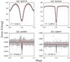 |
Fig. 1 Several examples of Kepler light curves and their respective model fits with polyfits and the two-Gaussian model. The plots show the observed Kepler light curve (gray dots) in normalized Kepler (K) magnitude, polyfit model (solid red line), and the two-Gaussian model (dashed black line). Magnitudes are obtained from the Kepler detrended flux and normalized to a reference value of 0 out of eclipse. |
Rate of eclipse identification by the two models on the set of 2861 phase-folded Kepler and Gaia-sampled light curves.
The eclipse detection overlap between the two models is given in Table 1. The two-Gaussian model fails to detect a primary eclipse for approximately 5% of the light curves. They are shown to correspond to very noisy light curves, where an actual eclipse is practically invisible, even if present. The primary eclipse detected by polyfits in these systems is negligible, and we conclude that the failure of the two-Gaussian model to detect it is not due to deficiencies of the model, but is governed by the data themselves. There is also a small portion (3.7%) of the light curves where the two-Gaussian model fails to detect a secondary eclipse. These are mainly attributed to very narrow secondary eclipses that do not contain many data points, and to eccentric binaries where the initial conditions are not suitable for the models to converge to a Gaussian at the position of the secondary eclipse. A relatively large number of cases (15.4%) have an identified secondary eclipse by the two-Gaussian model only, where a secondary Gaussian function has been fitted to the inter-eclipse variability. The differences in the model results are thus mainly a consequence of how each model adapts to the particular structure of the data. Examples of light curves that illustrate these discrepancies are given in Fig. 2.
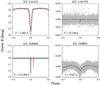 |
Fig. 2 Examples of Kepler light curves where the polyfit and the two-Gaussian model give discrepant results. The plots show the observed Kepler light curve (gray dots) in normalized Kepler (K) magnitude, polyfit model (solid red line), and two-Gaussian model (dashed black line). Top left: light curve where both models agree; top right: no primary eclipse detected by the two-Gaussian model; bottom left: no secondary eclipse detected by the two-Gaussian model; bottom right: no secondary eclipse detected by polyfit. |
For many of the cases the polyfit and two-Gaussian models look almost identical, but the underlying model parameters can differ greatly, in particular the eclipse widths. Polyfits compute them based on the positions of the knots in the polynomial chain (Prša et al. 2008), while the eclipse width in the two-Gaussian model corresponds to the widths of the Gaussian functions at a reference magnitude equal to 2% of the respective depth. For contact and ellipsoidal systems, which show continuous variability, the polynomial knots are usually positioned midway through the eclipses, resulting in a width of Δϕ ~ 0.25, while in the two-Gaussian model the eclipse width of these objects would typically saturate at Δϕ ~ 0.5 and is limited to Δϕ = 0.4. This disparity should be taken into account when comparing values from the two-Gaussian model and the polyfit values given in the Kepler Eclipsing Binaries catalog.
3.1.2. Gaia-sampled data
Unlike Kepler light curves, Gaia light curves have sparse (irregular) sampling. This introduces an additional difficulty to the models and is especially notable in polyfits, which in the absence of a well-defined light curve, tend to fit the polynomial chain to the out-of-eclipse noise. The two-Gaussian model, on the other hand, will either fit a constant model to the noise or produce a smooth curve resembling a physical light curve. This is a great advantage when dealing with light curves with well-defined eclipses, but noisy inter-eclipses, and for discarding cases where the points in an eclipse cannot be used for any quantitative analysis (bottom left panel of Fig. 3).
 |
Fig. 3 Same as Fig. 1, but for Gaia-sampled data. Top left: good quality data and both matching fits. Top right: good data, slightly discrepant fits. Bottom left: bad phase coverage in eclipse, the two-Gaussian model fits a constant model, while polyfits find eclipse. Bottom right: bad quality light curve and corresponding model fits. |
The eclipse identification rate with the two-Gaussian model on the Gaia-sampled data set again shows a loss of about 31.5% of the primary eclipse and an additional 16.8% of secondary eclipse identifications, which is a consequence of the deterioration of light curve quality. This gives an estimate of ~32% of Kepler eclipsing binaries that will likely not be identified with Gaia sampling. A summary of these results is given in Table 1.
3.2. Light curve classification
We use a combination of t-SNE and DBSCAN to classify a data set of M light curves, based on the per-point similarity of the phase-folded light curve models, computed in N phase points. Our Gaia-sampled Kepler data set consists of M = 2861 light curve models computed in N = 1000 equidistant phase points ranging from − 0.5 to 0.5 with imposed periodic boundary conditions. The input is an M × N array of the light curve model magnitudes. Each row is first rescaled so that its magnitudes span the range of [ 0,1 ]: 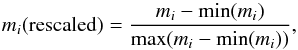 (1)where mi is the array of model magnitudes of the ith source in the input array. This ensures that the mapping is only sensitive to the light curve shape and is unaffected by the different primary eclipse depths. The rescaled magnitude array is first mapped to a three-dimensional map with t-SNE. The three-dimensional map serves as input to the second step of the mapping, in which a two-dimensional t-SNE map is produced. The two-dimensional t-SNE map is then scanned by DBSCAN, which defines a set of clusters and labels them, returning the per-point labels in a M × 1 array, which can be then assigned to the original input set of light curves. An illustration of the algorithm flow is given in Fig. 4.
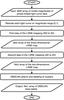 |
Fig. 4 Flowchart of the t-SNE+DBSCAN application to a set of M phase-folded light curve models computed in N equidistant phase points. |
3.2.1. Polyfit
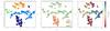 |
Fig. 5 t-SNE projection of the full Gaia-sampled data set fitted with polyfit models. Left panel: DBSCAN class flags; middle panel: manual fit quality flags; right panel: Kepler LLE morphology parameter distribution over the t-SNE projection. |
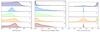 |
Fig. 6 Original Kepler value distributions of orbital period, Kepler primary eclipse depth, and eclipse separation over the different polyfit classes. Class descriptions are given in Table 2. |
We use the Barnes-Hut version of t-SNE (Van Der Maaten 2014) with perp3D = 50 and perp2D = 45 and DBSCAN with ε = 5 and MinPts = 50, which result in the identification of five polyfit clusters. The left panel of Fig. 5 shows the two-dimensional map color-coded by the detected DBSCAN classes. A visual inspection of the sources pertaining to each of the classes and their true Kepler polyfit parameters is used to define the descriptive classification provided in Table 2. It shows that the mapping has been driven by the morphology of the systems, ranging from close eclipsing binaries and ellipsoidal variables to detached systems, and by the relative depth of the eclipses. Phase-folding of the polyfit models has been performed with the known value of the zero-time reference point of primary eclipse obtained by Kepler light curves, which is why we get a class of sources with a more conspicuous secondary eclipse. Had this value not been provided to the model, classes 3 and 4 would have most likely been merged into one class of light curves with only one conspicuous eclipse, centered at orbital phase ϕ = 0. Classes 1 and 2 contain the close binary types – semi-detached (SD), contact binaries (CB), and ellipsoidal variables (ELV) – while class 0 contains the poor fits, i.e., polyfits that do not resemble a physical light curve.
DBSCAN results statistics for the polyfit models of the Gaia-sampled data set.
In addition to the automated approach, we performed a visual evaluation of each polyfit with three flags: good (g), medium (m), and bad (b) quality fit. Out of the 2861 sources, 1308 (46%) were marked as good, 770 (27%) as medium, and only 783 (27%) as bad. Actually, the DBSCAN class 0 contains ~93.6% of the visually flagged poor fits, ~6% of the medium quality, and only ~0.4% of good quality fits, which shows that class 0 is predominantly composed of the visually marked bad fits. The distribution of the flags over the t-SNE projection is given in the middle panel of Fig. 5. The distribution of the Kepler morphology parameter derived with LLE (Matijevič et al. 2012a; right panel of Fig. 5) shows the continuous transition from detached (morph = 0) to contact/ellipsoidal (morph = 1) binaries over the four classes containing good quality fits, while the poor polyfit class is shown to be mainly composed of detached systems, whose eclipses are likely not observed in Gaia cadences.
We use Kepler-derived parameters and quantities related to the quality of fits to search for indicators of the underlying causes for the bad data quality resulting in poor fits. The histograms of the orbital period, primary eclipse depth, and eclipse separation parameters over the different classes given in Fig. 6 show that class 0 is composed of both long- and short-period binaries and low to high eclipse depth values, but the low eclipse depth systems prevail. Based on these parameter distributions, we conclude that class 0 is composed of sources that will likely not show any eclipsing binary features, due to the possible miss of eclipse or low eclipse signal buried in the background noise. Classes 3 and 4 show similar parameter distributions, but their light curves have at least one prominent eclipse, thus we can consider those “lucky catch eclipses” that happen in Gaia cadences. The wider distributions of eclipse separation in classes 0, 3 and 4 show that they contain eccentric systems, as well as light curves where the secondary eclipse is not present (eclipse separation equal to 1). This similarity of class 0 to classes 3 and 4 further reinforces the necessity of a filtering approach primarily based on the light curve shape, since no threshold can be set to the values of any of the characteristic light curve parameters that would provide a clear distinction between poor and good quality fits.
3.2.2. Two-Gausssian
The two-Gaussian model has a built-in mechanism of identifying the light curves that do not show any eclipses through the choice of a constant as the best-fit model. Out of the 2861 Gaia-sampled light curves, 859 (about 30%) were fitted with a constant model; 575 (66%) of these light curves also belong to the bad polyfit class, while the remaining 34% primarily correspond to light curves with one or just a few data points in eclipses, which the two-Gaussian model flags as insignificant, while polyfit still fits an eclipse. Examples of these light curves are given in Fig. 7.
Proposed classification scheme for the two-Gaussian fits on Gaia-sampled Kepler data.
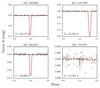 |
Fig. 7 Examples of Gaia-sampled light curves where the polyfit model fits an eclipse, while the two-Gaussian does not. The plots show the observed Kepler light curve (gray dots) in normalized Kepler (K) magnitude, polyfit model (solid red line), and two-Gaussian model (dashed black line). |
3.2.3. Filtered data set
The two-Gaussian model has a more thorough and consistent approach towards filtering data that is unlikely to pass Gaia’s eclipsing binary detection pipeline, thus we remove the 859 light curves fitted with the constant model and propose a classification scheme for the remaining 2002 sources. The application of t-SNE+DBSCAN with perp3D = 35, perp2D = 35, ε = 2.6, and MinPts = 18 on the two-Gaussian models results in nine classes (Fig. 8), marked from 1 to 9, that can be used to define a classification scheme based on the morphology of the systems and geometry of the light curve fits given in Table 3. Representative light curves for each class are given in Fig. 8.
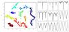 |
Fig. 8 Left panel: t-SNE+DBSCAN of filtered Gaia-sampled Kepler data set fitted with the two-Gaussian model. Right panel: mean of all normalized light curves in each DBSCAN class; gray shading indicates the region [−σ,σ ] around the computed mean at a given orbital phase. |
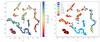 |
Fig. 9 Distributions of the LLE morphology parameter of Kepler EBs (left panel) and two-Gaussian models chosen to fit the light curves (right panel) over the t-SNE projection of the filtered Gaia-sampled Kepler data set fitted with the two-Gaussian model. |
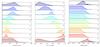 |
Fig. 10 Orbital period, LLE morphology parameter, and reduced χ2 distributions over different classes of the projection of the filtered two-Gaussian data set. |
Six main classes have been defined based on the light curve morphology, ranging from detached (D), detached and semi-detached (D+SD), semi-detached and contact binaries (SD+CB), contact binaries (CB), contact binaries and ellipsoidal variables (CB+ELV), and ellipsoidal fits (ELF). A clear distinction between overlapping morphological types among the different classes (D+SD, SD+CB, and CB+ELV) cannot be made because their light curve fits are intrinsically similar and the continuous transition from one morphological type to another is an inherent property of the light curve shapes. A more detailed distinction can be made through the inspection of the individual light curve properties, while in some cases full modeling of the system might be required for the accurate determination of its morphological type. The proposed morphological classes are thus an initial indication of the system morphology based on its light curve fit with the two-Gaussian model.
The subclasses are based on the geometrical properties of the light curves. The presence and visibility of eclipses define the subclasses in the detached and semi-detached classes: one conspicuous eclipse (D-1 and D+SD-1) or two conspicuous eclipses (D-2 and D+SD-2), while in the CB+ELV subclasses two eclipses are visible in most of the cases, thus the subclassification is driven by the eclipse or ellipsoidal variation widths and depths. In contact systems, the eclipse widths and depths can also be used as indicators of the physical system parameters, such as filling factor and temperature equilibrium. Wider eclipses, characteristic of classes 7 and 8, point to a larger filling factor, while similar eclipse depths, characteristic of classes 6 and 8, point to a system close to thermal equilibrium (e.g., a W UMa star).
The distribution of the Kepler LLE morphology parameter over classes (left panel of Fig. 9 and middle panel of Fig. 10), suggests that the proposed classification scheme corresponds to the morphological type of the observed sources determined on the true Kepler light curves. The orbital period distribution (left panel of Fig. 10) further supports this notion, with transitions from long periods in the detached to shorter periods in the semi-detached and contact classes.
The distribution of the different two-Gaussian model types over the projection (right panel of Fig. 9) shows that the projection is highly driven by the choice of the fitting model. This is expected since the model defines the light curve geometry, but the different widths and depths of the eclipses lead to mixing of the models in most of the classes, with the exception of class 9, which is composed solely of ellipsoidal fits.
The distribution of the reduced χ2 value (right panel of Fig. 10) is an indicator of the fit quality, which indirectly influences the classification. The classes corresponding to detached systems have both low and high reduced χ2, due to the small width and contribution of the eclipses to the overall light curve, while as we move towards closer systems with wider and more significant eclipses, the distributions are dominated by lower reduced χ2 values. This is a valuable indicator of the reliability of the light curve parameters provided for each class.
Class 9 shows the most peculiar parameter distributions of all, pertaining to both very low and very high values of the morphology parameter and predominantly higher reduced χ2 values. These indicate that class 9 is not only composed of ellipsoidal fits which correspond to true ellipsoidal variables, but also of detached systems where an eclipse has not been observed and the cosine function is fitted to the inter-eclipse scatter. This flags class 9 and the model parameters derived for the sources in it as unreliable and subject to further filtering.
4. Conclusions and future prospects
In this paper, we have presented for the first time a proposed method of automated reduction and classification of Gaia eclipsing binary data.
Results from both the analysis of the bad cases identified by the polyfits and the two-Gaussian model, and the comparison of eclipse detection rates of the two-Gaussian model applied to real Kepler and Gaia-sampled Kepler data, show that about 68% of all eclipsing binaries in the magnitude interval of Kepler are detectable by Gaia over a five-year mission. The orbital parameters and morphologies derived from the Kepler data show that the 32% non-detectable sources are mainly long-period detached binaries with very narrow eclipses that can easily be missed in the ~87 light curve points expected to be observed (on average) in Cygnus by Gaia over five years. Given that the all-sky average number of observations for Gaia is ~67, we expect the all-sky detectability to be lower than 68%. The other source types less likely to be detected include systems with very low eclipse depths that can easily be buried in the data noise.
We investigated the efficiency of the combined use of the t-SNE and DBSCAN algorithms to classify eclipsing binary light curves. The application to Kepler eclipsing binary light curves sampled at observation times predicted by the Gaia scanning law and characterized with the two-Gaussian model shows that the method is able to identify six broad classes corresponding to the system morphologies (detached, detached+semi-detached, semi-detached+contact binaries, contact binaries, contact binaries+ellipsoidal variables, and ellipsoidal fits).
An additional subclassification is introduced based on the properties of the fitted models (presence and visibility of eclipses and eclipse widths) to distinguish them from the physical properties of the observed systems that may not be correctly evaluated, due to the irregular sampling in Gaia observations; for example, systems with only one observed eclipse may in reality also have a prominent secondary eclipse that was not observed with Gaia’s scanning law.
The thorough testing, formulation, and implementation of automated reduction and classification techniques are of the highest priority in the Gaia era. One aspect of the method that is still open for adjustment on real Gaia data is its performance on data sets of much larger scale than used in this study. Several optimization approaches using parametric mapping between the high- and low-dimensional space (i.e., parameteric t-SNE) are being considered, as well as a combination of more than one classification approach (see Süveges et al. 2017). The final aim of this collaborative effort is to provide Gaia data archive users with a clean set of geometrical light curve parameters of eclipsing binaries, an estimate of their credibility, and classification types that would make the selection of a desired data subset as effortless and reliable as possible.
Alternative scanning laws were used during two months prior to the start of the Nominal Scanning Law (NSL), but they did not intersect with the Kepler field.
Acknowledgments
We are grateful to our referee Dr. J. A. Caballero for his constructive input, which substantially improved the quality and presentation of the paper. A.K. gratefully acknowledges the MSE postdoctoral fellowship of the College of Liberal Arts and Sciences at Villanova University.
References
- Auvergne, M., Bodin, P., Boisnard, L., et al. 2009, A&A, 506, 411 [NASA ADS] [CrossRef] [EDP Sciences] [Google Scholar]
- Borucki, W. J., Koch, D., Basri, G., et al. 2010, Science, 327, 977 [NASA ADS] [CrossRef] [PubMed] [Google Scholar]
- Caballero, J. A., & Dinis, L. 2008, Astron. Nachr., 329, 801 [NASA ADS] [CrossRef] [Google Scholar]
- Christiansen, J. L., Jenkins, J. M., Caldwell, D. A., et al. 2012, PASP, 124, 1279 [NASA ADS] [CrossRef] [Google Scholar]
- Dischler, J., & Söderhjelm, S. 2005, in The Three-Dimensional Universe with Gaia, eds. C. Turon, K. S. O’Flaherty, & M. A. C. Perryman, ESA SP, 576, 569 [Google Scholar]
- Ester, M., Kriegel, H., Sander, J., & Xu, X. 1996, in Proc. 2nd Int. Conf. on Knowledge Discovery and Data Mining (KDD’96) (AAAI Press), 226 [Google Scholar]
- Eyer, L., Holl, B., Pourbaix, D., et al. 2013, Central European Astrophysical Bulletin, 37, 115 [NASA ADS] [Google Scholar]
- Gaia Collaboration (Prusti, T., et al.) 2016, A&A, 595, A1 [NASA ADS] [CrossRef] [EDP Sciences] [Google Scholar]
- Holl, B., Lindegren, L., & Hobbs, D. 2012, A&A, 543, A15 [NASA ADS] [CrossRef] [EDP Sciences] [Google Scholar]
- Hotelling, H. 1933, J. Educational Psychology, 24, 417 [Google Scholar]
- Jordi, C., Gebran, M., Carrasco, J. M., et al. 2010, A&A, 523, A48 [NASA ADS] [CrossRef] [EDP Sciences] [Google Scholar]
- Kirk, B., Conroy, K., Prša, A., et al. 2016, AJ, 151, 68 [NASA ADS] [CrossRef] [Google Scholar]
- Matijevič, G., Prša, A., Orosz, J. A., et al. 2012a, AJ, 143, 123 [NASA ADS] [CrossRef] [Google Scholar]
- Matijevič, G., Zwitter, T., Bienaymé, O., et al. 2012b, ApJS, 200, 14 [NASA ADS] [CrossRef] [Google Scholar]
- Mowlavi, N., Lecoeur-Taïbi, I., Rimoldini, L., et al. 2017, A&A, accepted [Google Scholar]
- Perryman, M. A. C., Lindegren, L., Kovalevsky, J., et al. 1997, A&A, 323, 49 [Google Scholar]
- Perryman, M. A. C., de Boer, K. S., Gilmore, G., et al. 2001, A&A, 369, 339 [NASA ADS] [CrossRef] [EDP Sciences] [Google Scholar]
- Pojmanski, G. 2002, Acta Astron., 52, 397 [NASA ADS] [Google Scholar]
- Pribulla, T., Rucinski, S. M., Latham, D. W., et al. 2010, Astron. Nachr., 331, 397 [NASA ADS] [CrossRef] [Google Scholar]
- Prša, A., Guinan, E. F., Devinney, E. J., et al. 2008, ApJ, 687, 542 [NASA ADS] [CrossRef] [Google Scholar]
- Roweis, S. T., & Saul, L. K. 2000, Science, 290, 2323 [Google Scholar]
- Süveges, M., Barblan, F., Lecoeur-Taïbi, I., et al. 2017, A&A, accepted [Google Scholar]
- Thompson, S. E., Everett, M., Mullally, F., et al. 2012, ApJ, 753, 86 [Google Scholar]
- Udalski, A., Szymanski, M. K., Soszynski, I., & Poleski, R. 2008, Acta Astron., 58, 69 [NASA ADS] [Google Scholar]
- Van Der Maaten, L. 2014, J. Mach. Learn. Res., 15, 3221 [Google Scholar]
- Van Der Maaten, L., & Hinton, G. E. 2008, J. Mach. Learn. Res., 9, 2579 [Google Scholar]
- Zwitter, T. 2002, in Exotic Stars as Challenges to Evolution, eds. C. A. Tout & W. van Hamme, ASP Conf. Ser., 279, 31 [Google Scholar]
All Tables
Rate of eclipse identification by the two models on the set of 2861 phase-folded Kepler and Gaia-sampled light curves.
Proposed classification scheme for the two-Gaussian fits on Gaia-sampled Kepler data.
All Figures
|
Fig. 1 Several examples of Kepler light curves and their respective model fits with polyfits and the two-Gaussian model. The plots show the observed Kepler light curve (gray dots) in normalized Kepler (K) magnitude, polyfit model (solid red line), and the two-Gaussian model (dashed black line). Magnitudes are obtained from the Kepler detrended flux and normalized to a reference value of 0 out of eclipse. |
| In the text | |
|
Fig. 2 Examples of Kepler light curves where the polyfit and the two-Gaussian model give discrepant results. The plots show the observed Kepler light curve (gray dots) in normalized Kepler (K) magnitude, polyfit model (solid red line), and two-Gaussian model (dashed black line). Top left: light curve where both models agree; top right: no primary eclipse detected by the two-Gaussian model; bottom left: no secondary eclipse detected by the two-Gaussian model; bottom right: no secondary eclipse detected by polyfit. |
| In the text | |
|
Fig. 3 Same as Fig. 1, but for Gaia-sampled data. Top left: good quality data and both matching fits. Top right: good data, slightly discrepant fits. Bottom left: bad phase coverage in eclipse, the two-Gaussian model fits a constant model, while polyfits find eclipse. Bottom right: bad quality light curve and corresponding model fits. |
| In the text | |
|
Fig. 4 Flowchart of the t-SNE+DBSCAN application to a set of M phase-folded light curve models computed in N equidistant phase points. |
| In the text | |
|
Fig. 5 t-SNE projection of the full Gaia-sampled data set fitted with polyfit models. Left panel: DBSCAN class flags; middle panel: manual fit quality flags; right panel: Kepler LLE morphology parameter distribution over the t-SNE projection. |
| In the text | |
|
Fig. 6 Original Kepler value distributions of orbital period, Kepler primary eclipse depth, and eclipse separation over the different polyfit classes. Class descriptions are given in Table 2. |
| In the text | |
|
Fig. 7 Examples of Gaia-sampled light curves where the polyfit model fits an eclipse, while the two-Gaussian does not. The plots show the observed Kepler light curve (gray dots) in normalized Kepler (K) magnitude, polyfit model (solid red line), and two-Gaussian model (dashed black line). |
| In the text | |
|
Fig. 8 Left panel: t-SNE+DBSCAN of filtered Gaia-sampled Kepler data set fitted with the two-Gaussian model. Right panel: mean of all normalized light curves in each DBSCAN class; gray shading indicates the region [−σ,σ ] around the computed mean at a given orbital phase. |
| In the text | |
|
Fig. 9 Distributions of the LLE morphology parameter of Kepler EBs (left panel) and two-Gaussian models chosen to fit the light curves (right panel) over the t-SNE projection of the filtered Gaia-sampled Kepler data set fitted with the two-Gaussian model. |
| In the text | |
|
Fig. 10 Orbital period, LLE morphology parameter, and reduced χ2 distributions over different classes of the projection of the filtered two-Gaussian data set. |
| In the text | |
Current usage metrics show cumulative count of Article Views (full-text article views including HTML views, PDF and ePub downloads, according to the available data) and Abstracts Views on Vision4Press platform.
Data correspond to usage on the plateform after 2015. The current usage metrics is available 48-96 hours after online publication and is updated daily on week days.
Initial download of the metrics may take a while.