| Issue |
A&A
Volume 601, May 2017
|
|
|---|---|---|
| Article Number | A30 | |
| Number of page(s) | 14 | |
| Section | Extragalactic astronomy | |
| DOI | https://doi.org/10.1051/0004-6361/201629775 | |
| Published online | 25 April 2017 | |
Multiwavelength variability study and search for periodicity of PKS 1510–089
1 LERMA, Observatoire de Paris, CNRS, 61 avenue de l’Observatoire, 75014 Paris, France
e-mail: This email address is being protected from spambots. You need JavaScript enabled to view it.
2 Collège de France, 11 place Marcelin Berthelot, 75005 Paris, France
3 Laboratoire Lagrange, Université Côte d’Azur, Observatoire de la Côte d’Azur, CNRS, boulevard de l’Observatoire, CS 34229, 06304 Nice Cedex 4, France
4 Centre National d’Études Spatiales, CNES, 2 place Maurice Quentin, 75001 Paris, France
5 INAF–Istituto di Astrofisica Spaziale e Fisica Cosmica, Sezione di Bologna, via Gobetti 101, 40129 Bologna, Italy
6 Scuola Normale Superiore, Piazza dei Cavalieri 7, 56126 Pisa, Italy
7 INFN–Sezione di Pisa, Largo B. Pontecorvo 3, 56127 Pisa, Italy
8 INAF, Osservatorio Astronomico di Brera, via E. Bianchi 46, 23807 Merate (LC), Italy
9 INAF-IRA, via P. Gobetti 101, 40129 Bologna, Italy
10 Dipartimento di Fisica e Astronomia, Università degli Studi di Bologna, Viale Berti Pichat 6/2, 40127 Bologna, Italy
11 Nordic Optical Telescope, Apartado 474, 38700 Santa Cruz de La Palma, Spain
12 INAF–Istituto di Astrofisica e Planetologia Spaziali, via Fosso del Cavaliere 100, 00133 Roma, Italy
13 CNRS/IN2P3, 3 rue Michel-Ange, 75794 Paris Cedex 16, France
14 INAF-IASF Palermo, via Ugo La Malfa 143, 90146 Palermo, Italy
15 INAF, Osservatorio Astrofisico di Torino, via Osservatorio 20, 10025 Pino Torinese (TO), Italy
16 Centre François Arago, APC, Université Paris Diderot, CNRS/IN2P3, 10 rue Alice Domon et Léonie Duquet, 75205 Paris Cedex 13, France
17 Università degli Studi dell’Insubria, via Valleggio 11, 22100 Como, Italy
18 INTEGRAL Science Data Centre, University of Geneva, Chemin d’Écogia 16, 1290 Versoix, Switzerland
Received: 22 September 2016
Accepted: 15 December 2016
Abstract
Context. Blazars are the most luminous and variable active galactic nuclei (AGNs). They are thus excellent probes of accretion and emission processes close to the central engine.
Aims. We concentrate here on PKS 1510–089 (z = 0.36), a blazar belonging to the flat-spectrum radio quasar subclass, an extremely powerful gamma-ray source and one of the brightest in the Fermi-LAT catalog. We aim to study the complex variability of this blazar’s bright multiwavelength spectrum, to identify the physical parameters responsible for the variations and the timescales of possible recurrence and quasi-periodicity at high energies.
Methods. The blazar PKS 1510–089 was observed twice in hard X-rays with the IBIS instrument onboard INTEGRAL during the flares of Jan. 2009 and Jan. 2010, and simultaneously with Swift and the Nordic Optical Telescope (NOT), in addition to the constant Fermi monitoring. We also measured the optical polarization in several bands on 18 Jan. 2010 at the NOT.Using these and archival data we constructed historical light curves at gamma-to-radio wavelengths covering nearly 20 yr and applied tests of fractional and correlated variability. We assembled spectral energy distributions (SEDs) based on these data and compared them with those at two previous epochs, by applying a model based on synchrotron and inverse Compton radiation from blazars.
Results. The modeling of the SEDs suggests that the physical quantities that undergo the largest variations are the total power injected into the emitting region and the random Lorentz factor of the electron distribution cooling break, that are higher in the higher gamma-ray states. This suggests a correlation of the injected power with enhanced activity of the acceleration mechanism. The cooling likely takes place at a distance of ~1000 Schwarzschild radii(~0.03 pc) from the central engine – a distance muchsmaller than the broad line region (BLR) radius.The emission at a few hundred GeV can be reproduced with inverse Compton scattering of highly relativistic electrons off far-infrared photons if these are located much farther than the BLR, that is, around 0.2 pc from the AGN, presumably in a dusty torus. We determine a luminosity of the thermal component due to the inner accretion disk of Ld ≃ 5.9 × 1045 erg s-1, a BLR luminosity of LBLR ≃ 5.3 × 1044 erg s-1, and a mass of the central black hole of MBH ≃ 3 × 10⁸ M⊙.The fractional variability as a function of wavelength follows the trend expected if X- and gamma-rays are produced by the same electrons as radio and optical photons, respectively.Discrete correlation function (DCF) analysis between the long-term Steward observatory optical V-band and gamma-ray Fermi-LAT light curves yields a good correlation with no measurable delay. Marginal correlation where X-ray photons lag both optical and gamma-ray ones by time lags between 50 and 300 days is found with the DCF.Our time analysis of the RXTE PCA and Fermi-LAT light curves reveals no obvious (quasi-)periodicities, at least up to the maximum timescale (a few years) probed by the light curves, which are severely affected by red noise.
Key words: galaxies: active / radiation mechanisms: general / quasars: individual: PKS 1510-089 / gamma rays: galaxies
© ESO, 2017
1. Introduction
Blazars are among the most luminous persistent extragalactic multiwavelength sources in the Universe. Their gamma-ray radiation is likely produced within hundreds to a few thousands of Schwarzschild radii of the central engine (Finke & Dermer 2010; Ghisellini et al. 2010; Tavecchio et al. 2010) or at the location of the circum-nuclear dust at parsec scales (Marscher et al. 2008, 2010; Sikora et al. 2009). Therefore blazar variability on a range of timescales from years down to hours is one of the most powerful diagnostic of their emission geometry and mechanisms (see e.g., Böttcher & Chiang 2002; Böttcher & Dermer 2010; Hayashida et al. 2012; Falomo et al. 2014; Dermer et al. 2014; Pian et al. 2014; Chidiac et al. 2016; Krauß et al. 2016).
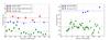 |
Fig. 1 Normalized light curves in observer frame during Jan. 2009 (left) and Jan. 2010 (right). Swift XRT (0.3–10 keV) data, corrected for Galactic HI absorption, are filled circles (blue); diamonds (red) are INTEGRAL IBIS/ISGRI (20–100 keV) data; squares (green) represent the Fermi-LAT (0.1–300 GeV) data daily-binned light curves, including 90% upper limits. All light curves are normalized with respect to their mean (computed without considering upper limits).For each light curve the dashed horizontal line shows the average normalized flux. Swift XRT and INTEGRAL normalized light curves are shifted up by constants two and three, respectively. |
The blazar PKS 1510–089 is a nearby (z = 0.36), variable, highly polarized flat-spectrum radio quasar (FSRQ, Burbidge & Kinman 1966; Stockman et al. 1984; Hewitt & Burbidge 1993), well monitored at all bands from the radio to gamma rays (e.g., Malkan & Moore 1986; Thompson et al. 1993; Pian & Treves 1993; Sambruna et al. 1994; Lawson & Turner 1997; Singh et al. 1997; Siebert et al. 1998; Tavecchio et al. 2000; Dai et al. 2001; Gambill et al. 2003; Wu et al. 2005; Bach et al. 2007; Li & Fan 2007; Kataoka et al. 2008; Nieppola et al. 2008). It is one of the brightest and most variable blazars detected by Fermi-LAT (Abdo et al. 2009, 2010a,d; Foschini et al. 2013; Ackermann et al. 2015a) and AGILE-GRID (Pucella et al. 2008; D’Ammando et al. 2009, 2011), and one of the only six FSRQs detected at very high energies – up to a few hundred GeV in the observer frame – with 3C 279, 4C 21.35, PKS 1441 +25,S3 0218+35, and PKS 0736+017 (Cohen et al. 2003; Albert et al. 2008; Aleksić et al. 2011; HESS Collaboration 2013; Abeysekara et al. 2015; Ahnen et al. 2015; Cerruti et al. 2016). For these reasons, it was the target of many recent multiwavelength observing campaigns, some of which included monitoring of its highly variable optical polarization (e.g., Rani et al. 2010; Abdo et al. 2010b,c; Marscher et al. 2010; Ghisellini et al. 2010; Sasada et al. 2011; Orienti et al. 2011, 2013; Arshakian et al. 2012; Stroh & Falcone 2013; Aleksić et al. 2014; Fuhrmann et al. 2016). This rich dataset became a benchmark for phenomenological studies of PKS 1510–089 (e.g., Kushwaha et al. 2016), theoretical modeling of its light curves (Tavecchio et al. 2010; Brown et al. 2013; Cabrera et al. 2013; Nakagawa & Mori 2013; Nalewajko 2013; Saito et al. 2013; Vovk & Neronov 2013; Marscher 2014; Dotson et al. 2015; MacDonald et al. 2015; Kohler & Nalewajko 2015), and spectral energy distributions (SEDs, Abdo et al. 2010c; Chen et al. 2012; Nalewajko et al. 2012, 2014; Yanet al. 2012; Böttcher et al. 2013; Barnacka et al. 2014; Saito et al. 2015; Böttcher & Els 2016; Basumallick et al. 2017).
Evidence for possible year timescale periodicity of PKS 1510–089 was foundfrom the radio to gamma rays (e.g., Xie et al. 2008; Abdo et al. 2010c; Castignani 2010; Sandrinelli et al. 2016). The search for quasi-periodicities in light curves (e.g., Valtonen et al. 2008, 2011; Zhang et al. 2014; Sandrinelli et al. 2014a,b; Graham et al. 2015a,b; Ackermann et al. 2015b) and spectra (e.g., Tsalmantza et al. 2011; Ju et al. 2013; Shen et al. 2013) of active galactic nuclei (AGNs) is a long-standing issue because it is related to the possible presence of close binary systems of supermassive black holes (SMBHs) and received recent boost from the relevance of these systems as potential sources of milli-Hz gravitational waves (Amaro-Seoane et al. 2013; Colpi 2014).
Because of its characteristics, PKS 1510–089 is a prominent target for our program of INTEGRAL observations of blazars in outburst. The source was first observed by INTEGRAL IBIS in 2008 (Barnacka & Moderski 2009) and detected with a hard X-ray flux that was about a factor of two lower than observed by Suzaku in 2006 (Kataoka et al. 2008). We have re-observed it during high states in Jan. 2009 and Jan. 2010, and report here a study of its multiwavelength light curves and spectra at various epochs, based on the INTEGRAL data and quasi-simultaneous observations made with the Swift satellite (some of which are presented here for the first time), Fermi-LAT and with the Nordic Optical Telescope (NOT). In order to put our data in the context of the long-term behavior of PKS 1510–089 we have also retrieved from the archive and the literaturegamma-ray (EGRET, Fermi, and AGILE), optical (Steward Observatory and the Rapid Eye Mount telescope), and radio (MOJAVE VLBA program) data of this source. Moreover, we have reanalyzed the RXTE PCA dataset of PKS 1510–089 up to April 2011 and present a timing analysis of this light curve in search of periodicity using several independent methods. We also present models of the SEDs that we have elaborated to identify the main parameters that are responsible for the multiwavelength long-term variability.
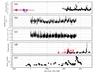 |
Fig. 2 Historical light curves in observer frame. a) Gamma-ray light curve. The small filled circles (black) represent the Fermi-LAT (0.1–300 GeV) weekly-binned light curve; the 90% confidence upper limits are also reported; crosses and big upper limits (blue) represent the CGRO-EGRET (>100 MeV) fluxes from 3rd EGRET catalog (Hartman et al. 1999); squares (red) are the CGRO-EGRET fluxes from the revised EGRET catalog (Casandjian & Grenier 2008); diamonds (green) are AGILE-GRID (>100 MeV) detections (Pucella et al. 2008; D’Ammando et al. 2009; Striani et al. 2010). b) X-ray Rossi XTE light curve (2–15 keV) and 3σ upper limits.The average (median) separation between consecutive observations, once upper limits are removed, is 4.2 ± 6.5 days (3.4 days). The reported uncertainty is the rms dispersion. c) X-ray Rossi XTE hardness ratio(7.5–15 keV vs. 2–7.5 keV channels). d) Optical V-band historical light curve, corrected for Galactic dust absorption (EB−V = 0.09, Schlafly & Finkbeiner 2011), using the extinction curve from Cardelli et al. (1989). The REM observations (red crosses) are from (Sandrinelli et al. 2014a); the black circles represent photometry obtained at the Steward Observatory (Smith et al. 2009); the blue squares are our NOT data (Table 3). e) Radio VLBA I-band (15 GHz) light curve from the MOJAVE database (Lister et al. 2009). |
Throughout this work we have adopted a flat ΛCDM cosmology with matter density Ωm = 0.30, dark energy density ΩΛ = 0.70 and Hubble constant h = H0/ 100 km s-1 Mpc-1 = 0.70 (see however, Planck Collaboration XIII 2016; Riess et al. 2016). Under these assumptions the luminosity distance of PKS 1510–089 is 2.0 Gpc.
In Sect. 2 we report the observations of our campaigns, the data analysis, and the results. In Sect. 3 we describe the multiwavelength variability and cross-correlation among light curves, and present the results of our periodicity search. Section 4 reports on multi-epoch SED construction and modeling. In Sect. 5 we draw our conclusions.
2. Observations, data analysis and results
Our INTEGRAL program for blazars in outburst as Targets of Opportunity was activated in 2009 following a notification of a rapid GeV flare of PKS 1510–089 detected by the LAT instrument on board the Fermi gamma-ray satellite on Jan. 8, 2009 (Ciprini & Corbel 2009; Abdo et al. 2010c), and again in 2010 after the detection of an outburst at E > 100 MeV with the GRID instrument on-board AGILE on Jan. 11–13, 2010 (Striani et al. 2010). Multiwavelength observations with the Swift satellite and the NOT were coordinated quasi-simultaneously with the INTEGRAL campaign. RXTE PCA and Fermi-LAT data retrieved from the archive were also used to study the variability over an extended time interval. In the following we describe the data reduction and analysis of the multiwavelength data.
In Fig. 1 we report the high-energy light curves of the 2009 and 2010 campaigns and in Fig. 2 the historical multiwavelength light curves.The INTEGRAL IBIS/ISGRI data of Jan. 2010 have sufficient signal-to-noise ratio to produce an integrated spectrum, but not a light curve. Therefore they are not plotted in the right panel of Fig. 1. In the following sub-sections we will present the gamma-ray-to-optical data. The radio light curve (Fig. 2e) is from VLBA measurements in I-band (15 GHz) downloaded from the MOJAVE database1.
2.1. Gamma-rays
Gamma-ray data of PKS 1510–089 were downloaded from the Fermi-LAT public archive2 in the form of weekly- and daily-binned light curves. In panel a of Fig. 2 we show the 0.1–300 GeV weekly-binned, approximately eight-year long Fermi-LAT light curve, where flux measurements are reported along with 90% upper limits. EGRET (>100 MeV) data (Hartman et al. 1999; Casandjian & Grenier 2008) and AGILE-GRID observations of summer 2007 (Pucella et al. 2008) and March 2008 (D’Ammando et al. 2009) are also reported. The daily-binned Fermi-LAT 0.1–300 GeV light curves during the flaring periods of 2009 and 2010 (Jan. 11, 2009–Feb. 1, 2009 and Dec. 26, 2009–Jan. 23, 2010) are reported in Fig. 1, along with X-ray light curves from Swift XRT and INTEGRAL (see Sect. 2.2).
The historical light curve shows that the gamma-ray activity has increased during the years from the EGRET to Fermi era up to a factor of approximately eight, thus making PKS 1510–089 one of the brightest Fermi-LAT monitored blazar.
Swift XRT observations in Jan. 2010.
Swift UVOT photometry in Jan. 2010.
2.2. X-rays
The INTEGRAL satellite (Winkler et al. 2003) observed PKS 1510–089 in a non-continuous way starting on 2009 Jan. 11, 15:14:28 UT and ending on 2009 Jan. 24, 15:02:44 UT (revolutions 763 to 767), and again between 2010 Jan. 17, 14:15:10 UT and 2010 Jan. 19, 2010, 04:16:49 UT (revolution 887). A 5 × 5 dither pattern was adopted, so that the total on-source exposure time of the IBIS/ISGRI instrument (Ubertini et al. 2003; Lebrun et al. 2003) was 405 ks in 2009 and 95 ks in 2010.
Screening, reduction, and analysis of the INTEGRAL data were performed using the INTEGRAL Offline Scientific Analysis (OSA) V. 10.1 and IC V. 7.0.2 for calibration, both publicly available through the INTEGRAL Science Data Center3 (ISDC, Courvoisier et al. 2003). The algorithms implemented in the software are described in Goldwurm et al. (2003) for IBIS, Westergaard et al. (2003) for JEM-X, and Diehl et al. (2003) for SPI. The IBIS/ISGRI, SPI, and JEM-X data were accumulated into final images. For the spectral analysis we used the matrices available in OSA (V. 10.1).
In 2009 IBIS/ISGRI detected PKS 1510–089 up to E = 100 keV with an average count rate in the coadded image of 0.39 ± 0.05 counts s-1 in the energy range 20–100 keV. The spectrum in this energy range is well fit by a single power-law FE ∝ E− Γ with photon index Γ = 1.7 ± 0.6 and the flux is (3.4 ± 0.9) × 10-11 erg cm-2 s-1.The relatively low Galactic absorption, NH = 7 × 1020 cm-2 (Kalberla et al. 2005), is not influential at these energies. The 2010 IBIS/ISGRI average count rate in the coadded image is 0.83 ± 0.08 counts s-1 (20–100 keV). The spectrum has a photon index  and a flux of (6.2 ± 1.4) × 10-11 erg cm-2 s-1. The IBIS/PICsIT, SPI and JEM-X instruments on-board INTEGRAL have not detected the source at either epoch.
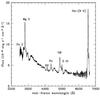 |
Fig. 3 Rest frame optical spectrum taken at the NOT with ALFOSC on 22 Feb. 2009 and corrected for Galactic extinction (EB−V = 0.09). The most prominent emission lines are labeled. Some fringing(removed in the figure) affects the spectrum long-ward of ~5600 Å. |
The blazar PKS 1510–089 was observed with the Swift XRT (Burrows et al. 2005) in Jan. 2009 (Abdo et al. 2010c; D’Ammando et al. 2011) and four times in Jan. 2010 (see Table 1). The data reduction and analysis of the 2009 data was presented in Abdo et al. (2010c). The 2010 data were processed following usual procedures as detailed, for example, in D’Ammando et al. (2009, 2011), that is, the source events were extracted in circular regions centered on the source with radii depending on the source intensity (10–20 pixels, 1 pixel ~2.37 arcsec), while background events were extracted in source-free annular or circular regions. Given the low count rate (<0.5 counts s-1), we only considered photon counting (PC) data and further selected XRT grades 0–12. No pile-up correction was required. The data were deabsorbed assuming Galactic HI column density NH = 7 × 1020 cm-2 (Kalberla et al. 2005). XRT spectra were extracted for each observation. Ancillary response files, accounting for different extraction regions, vignetting, and point spread function (PSF) corrections, were generated with xrtmkarf. We used the spectral redistribution matrices in the Calibration Database maintained by HEASARC. All spectra were rebinned with a minimum of 20 counts per energy bin to allow χ2 fitting within xspec (v11.3.2) and fit to single power-laws whose indices are reported in Table 1.
NOT photometry.
The RXTE satellite observed PKS 1510–089 from 1996 to 2012 with the PCA instrument. Count rates in the 2–15 keV band were retrieved from the archive and corrected for the background. Light curves were produced in two bands (A and B, covering approximately the 2–7.5 keV and 7.5–15 keV, respectively, with some dependence of these bands on mission lifetime).
In panel b of Fig. 2 we report the sum of the rates in A and B bands (so called C band, 2–15 keV) and 3σ upper limits, with no correction applied for the negligible neutral hydrogen column density. In panel c we report the hardness ratio B/A. To improve the statistics we limit our long-term variability analysis to the C-channel only (see Sect. 3).
2.3. Near-infrared-optical-ultraviolet
Swift UVOT (Roming et al. 2005) data acquired in Jan. 2010 were reduced following procedures adopted in previous observations (D’Ammando et al. 2009, 2011). Counts-to-magnitudes conversion factors from Poole et al. (2008) and Breeveld et al. (2011) were assumed4. The resulting UVOT magnitudes are reported in Table 2.
We observed the target in Jan. 2009 and Jan. 2010 with the StanCam, NOTCam and ALFOSC cameras and optical and near infrared (NIR) filters at the 2.5 m NOT located on La Palma. The data were reduced following standard procedures within the IRAF package (Tody 1986, 1993). A bias subtraction, pixel-to-pixel flat fielding using the normalized internal Halogen data, and wavelength calibration using internal HeNe-lamp were applied to the raw images. Aperture photometry was performed with the IRAF5 routine APPHOT and calibrated using a standard photometric sequence6. Various comparison stars were used depending on filter. The NOT magnitudes (in Bessel system, except the i-band which is in AB system) are reported in Table 3 and in Fig. 2d.
The 60 cm diameter Rapid Eye Mount (REM) telescope at the ESO site of La Silla observed PKS 1510–089 between April 2005 and June 2012 in VRIJHK filters. We report in panel d of Fig. 2 the REM V-band light curve from Sandrinelli et al. (2014a) as well as the V-band archival photometry obtained at the Steward Observatory (Smith et al. 2009). For both light curves, the relation VJohnson = VAB + 0.044 is used to convert V-band Johnson-Cousins (VJohnson) to AB (VAB) magnitudes (Frei & Gunn 1994).
On 18 Jan. 2010 we acquired polarimetry of the source in several bands with ALFOSC (exposure time of 100 s). The polarized percentages, reported in Table 4, were obtained using an aperture radius of 2 arcsec for band B and 3 arcsec for bands z, i, and V. While the polarization percentage increases with wavelength, the polarization angle, once systematic uncertainties ~10% for the latter are taken into account, stays constant within the errors.
A spectrum of the source was taken on 22 Feb. 2009 with ALFOSC and reduced following standard procedures within the IRAF package (Tody 1986, 1993). The data were reduced following standard procedures within the IRAF (overscan subtraction, bias correction, twilight flat fielding). Aperture photometry was done with the IRAF routine APPHOT. The spectrum (Fig. 3) shows several bright emission lines as well as evidence of a “small blue bump” due to the blending of iron lines, often detected in AGNs in the rest frame range ~2200–4000 Å (Wills et al. 1985; Elvis 1985). The sum of the luminosities of the six most luminous emission lines (Hα, Hβ+OIII, Hγ, Hδ, MgII, FeII) yields Llines = 2.3 × 1044 erg s-1. Following Francis et al. (1991), we correct for the presence of unobserved lines, in particular the Lyα+NV blend, which is expected to contribute significantly to the total line emission, since its observed flux is 0.88 × 10⁻¹³ erg s-1 cm-2 (Osmer et al. 1994), i.e., ~50% brighter than Hα when reddening is taken into account. We find that the estimated broad line region (BLR) luminosity is LBLR = 5.3 × 1044 erg s-1 which is consistent within a factor of ~2, and considering its year timescale variability (Isler et al. 2015), with LBLR = 7.4 × 1044 erg s-1 reported by Celotti et al. (1997). The estimated LBLR is a factor of seven less than the assumed disk luminosity (see Sect. 4.2), consistent with a BLR-to-disk covering factor ~1/10 assumed in previous work (Böttcher & Els 2016).
3. Multiwavelength variability
3.1. Variability amplitude
The hard X-ray flux (10–50 keV) of PKS 1510–089 varies altogether by nearly a factor of 3 during the period going from Aug. 2006, when Suzaku observed it to be ~3.8 × 10⁻¹¹ erg s-1 cm-2 (Kataoka et al. 2008), to the first INTEGRAL IBIS observation in Jan. 2008 (~1.6 × 10⁻¹¹ erg s-1 cm-2, Barnacka & Moderski 2009), and our IBIS observations in Jan. 2009 (~2.8 × 10⁻¹¹ erg s-1 cm-2) and Jan. 2010 (4.1 × 10⁻¹¹ erg s-1 cm-2, see Sect. 2.2). In Jan. 2009 it shows daily variability by about a factor of ~2 during our campaign, while the soft X-ray (0.3–10 keV) flux varies by at most 30–40%, and the gamma-ray flux varies by a factor of approximately five (Fig. 1, left). In Jan. 2010, the MeV-GeV flux is about at the same level as in Jan. 2009 and varies with similar amplitude, while the soft X-ray flux varies by a factor of approximately two, although on average it is at the same level as in Jan. 2009 (Fig. 1, right). These results indicate a complex behavior in the X-ray and gamma-ray correlated light curves on timescales from years down to days and suggest that different components drive the variability at the different epochs.
We then considered the multiwavelength historical light curves (Fig. 2) and evaluated the fractional variability at all wavelengths following Fossati et al. (2000), Vaughan et al. (2003). In doing so, we conservatively discarded the 90% Fermi-LAT and 3σ RXTE PCA upper limits. The results are reported in Table 5 and indicate that the variability amplitude is wavelength-dependent, but not monotonic. It increases between radio and optical, but at X-rays is similar to that at radio wavelengths, and it reaches a maximum at gamma-rays. This is in line with what is observed in the individual epochs (Sandrinelli et al. 2014a; Kushwaha et al. 2016), and with the general behavior of flat-spectrum radio quasars, where the radio-to-ultraviolet and X-ray-to-gamma-ray parts of the spectrum are dominated by different components, synchrotron emission and inverse Compton scattering, respectively, that are however correlated (Wehrle et al. 1998; Vercellone et al. 2011; Pian et al. 2011; Tavecchio et al. 2013). In view of this and of the lack of a clear pattern in the high energy variability, we have cross-correlated the long-term gamma-ray, X-ray, optical,and radio light curves in search of possible delays.
NOT polarization measurements of 18 Jan. 2010.
Fractional rms variability amplitude for the historical light curves.
3.2. Cross-correlation
We have applied the discrete correlation function (DCF, Edelson & Krolik 1988), which is widely used to estimate cross- and auto-correlations of unevenly sampled data of AGNs (Urry et al. 1997; Kaspi et al. 2000; Raiteri et al. 2001; Onken & Peterson 2002; Zhang et al. 2002; Abdo et al. 2010d; Ackermann et al. 2011; Agudo et al. 2011). We have considered pairwise the gamma-ray (Fermi-LAT, 0.1–300 GeV), X-ray (RXTE PCA, 2–15 keV), optical (Steward Observatory V-band), and radio (MOJAVE VLBA, 15 GHz) light curves within their common time range, that is, between 4411.5 and 5508.1 days from 1 Dec. 1996. Within this time range the mean (median) time separations of consecutive observations for the four light curves are 7.6 ± 2.5 days (7.0 days), 2.8 ± 5.3 days (2.0 days), 9.4 ± 24.0 days (1.0 days), and 50.6 ± 30.9 days (54.0 days), respectively. The uncertainties denote the rms dispersion. The DCF time bin was chosen to be approximately three times larger than the average time resolution of the worse sampled light curve and DCF time lags are considered as significant if they are at least three times larger than the adopted DCF time bin (see Edelson & Krolik 1988; Castignani et al. 2014). The resulting six DCFs are shown in Fig. 4. Positive time lags correspond to higher energy photons lagging lower energy photons.
We have also computed the DCF in the maximum time range of the two light curves considered in each panel, but this yields a significantly different result with respect to the above DCFs only for the optical and gamma-ray light curves (Fig. 4b): the DCF maximum at +300 days time lag disappears. Since the time range considered with the latter case (4411.5 and 7175.2 days from 1 Dec. 1996) is larger than in the former case, we deem this result more statistically significant, and therefore we dismiss the 300 days time lag determined in the former case.
In the gamma-ray vs. optical DCF (Fig. 4b) marginal correlation at zero time lag is observed. A zero time lag between optical and gamma-ray photonsis consistent with the delays found by Abdo et al. (2010c) and Nalewajko et al. (2012) over a different time interval (13 days, zero time lag, and 25 days) if one considers that our time-resolution is approximately one week and approximately nine days for the gamma-ray and optical light curves, respectively.Similar time delays consistent with zero between the optical and the gamma-ray photons have been found also in other FSRQs such as 3C 454.3 (Bonning et al. 2009; Gaur et al. 2012; Kushwaha et al. 2017).
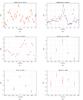 |
Fig. 4 DCF curves between pairs of gamma-ray (Fermi-LAT, 0.1–300 GeV), X-ray (RXTE PCA, 2–15 keV), optical (Steward Observatory V-band), and radio (15 GHz) light curves considered in their common time range, i.e., between 4411.5 and 5508.1 days from 1 Dec. 1996 (orange circles and solid error bars). In panel b), we have reported as blue circles and dashed error bars also the DCF obtained by considering the optical and gamma-ray light curves within their maximum common time range, i.e., between 4411.5 and 7175.2 days from 1 Dec. 1996. The reported errors are the statistical 1σ uncertainties. The DCF time bin adopted is equal to 20 days a), 30 days (b), c)), and 150 days (d), e), f)) and it is approximately equal to three times the mean time separation between consecutive observations of the light curve with the worse sampling. In each panel positive time lags correspond to variations of the lower-energy light curve preceding those of the higher-energy light curve. |
The gamma-ray versus X-ray DCF (Fig. 4a) and the X-ray versus optical DCF (Fig. 4c) suggest that the X-rays lag both the gamma-rays and the optical by an observed time interval of between 50 and 300 days. While this may be compatible with the fact that the gamma-rays and optical are produced in the same region by the synchrotron and inverse Compton cooling, respectively, of the same electrons (see also lack of time delay between optical and gamma-rays, Fig. 4b), the long delay of the X-rays (about 40 to 200 days in rest-frame) with respect to gamma-rays is difficult to reconcile with a physical timescale (see Hayashida et al. 2012, for discussion of this point), although it is generally in agreement with the fact that the X-rays may be produced in a more external region with respect to the innermost part of the jet.
The small amplitude of the gamma-ray versus X-ray DCF makes our results consistent with those of Abdo et al. (2010c), who did not find any robust evidence of cross-correlation between X- and gamma-rays for PKS 1510-089 at zero time lag during a shorter period (11 months) than examined here. Correlation of X-rays with optical was not reported in previous studies of FSRQs (e.g., Bonning et al. 2009; Gaur et al. 2012).
The poor sampling of the radio light curves prevents us to draw firm conclusions on the corresponding DCFs with emission at shorter wavelengths (Figs. 4d, e, f). We also checked that our results are independent of the adopted Fermi-LAT band and that they do not change significantly if both REM and Steward Observatory V-band light curves are altogether considered.We performed the cross-correlation analysis using the z-transformed DCF (zDCF, Alexander 1997, 2013) and found results entirely consistent with those obtained with the DCF.
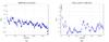 |
Fig. 5 Auto-correlation function(DCF) of the X-ray(RXTE PCA, 2–15 keV, left) and gamma-ray(Fermi-LAT, 0.1–300 GeV, right) light curves.DCF time bins of 13 and 20 days are adopted, respectively. The reported errors are the statistical 1σ uncertainties. |
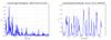 |
Fig. 6 Generalized Lomb-Scargle periodograms (Zechmeister & Kürster 2009) for the X-ray(RXTE PCA, 2–15 keV, left) and gamma-ray(Fermi-LAT, 0.1–300 GeV, right) light curves. |
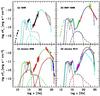 |
Fig. 7 Simultaneous or quasi-simultaneous multiwavelength spectra of PKS 1510–089 at different epochs in the rest frame. Soft X-ray data and ultraviolet-to-NIR data were corrected for neutral hydrogen absorption (NH = 7 × 1020 cm-2) and dust extinction (EB−V = 0.09) in our Galaxy, respectively. a) The filled black circles are from Kataoka et al. (2008) and refer to August 2006. Red bow-ties are archival data from ROSAT (Siebert et al. 1996), and CGRO-EGRET (>100 MeV, Apr. 1991–Nov. 1992, Hartman et al. 1999). b) Orange symbols are AGILE-GRID and GASP data obtained during 27 Aug.–1 Sep. 2007 (Pucella et al. 2008). Light green symbols are AGILE-GRID, GASP, Swift UVOT, and Swift XRT data of March 2008 (D’Ammando et al. 2009). The red bow-tie at hard X-ray frequencies corresponds to the INTEGRAL spectrum in Jan. 2008 (Barnacka & Moderski 2009). The red bow-tie at gamma-ray frequencies corresponds to Fermi-LAT observations during Aug.–Oct. 2008 (Abdo et al. 2009). c) Red symbols refer to optical data from NOT (13 and 18 Jan. 2009); Swift XRT and UVOT (10–25 Jan. 2009, Abdo et al. 2010c); INTEGRAL IBIS-ISGRI (13–24 Jan. 2009); Fermi-LAT data (10 Jan.–1 Feb. 2009). Blue symbols are HESS observations in March 2009 (HESS Collaboration 2013); upper limits at 3σ confidence for the two highest-energy bands are reported. d) Magenta symbols refer to optical data from NOT (23 Jan. 2010) and Swift/UVOT (15, 17, and 19 Jan. 2010); Swift XRT (15–19 Jan. 2010), INTEGRAL IBIS-ISGRI (17–19 Jan. 2010); and Fermi-LAT (26 Dec. 2009–23 Jan. 2010). The green symbol is the E > 100 MeV gamma-ray observation from AGILE (11–13 Jan. 2010, Striani et al. 2010). The black solid segment shows the polarized NOT spectrum of 18 Jan. 2010. Fluxes have been multiplied by a constant factor of 50. In each panel, we report the curves obtained from a fit of the SEDs with the blazar model (Ghisellini & Tavecchio 2009). The black dotted curve represents a thermal component that is assumed to be constant in time and consisting of radiation from an accretion disk (optical-ultraviolet), a torus (FIR) and a corona (X-rays, with an exponential cutoff at ~100 keV). The dot-dashed curve shows the synchrotron emission component. The dashed curve represents first and second order synchrotron self-Compton process. Most of the inverse Compton scattering occurs off external BLR photons (this individual component is not shown). The sum of the thermal and non-thermal components is shown as a single curve in each panel: cyan in a); blue in b); green in c) and red in d); where we report also the best-fit curves for the 3 previous epochs. The quasi-simultaneous VHE emission of Mar 2009 is modeled independently by external Compton of infrared photons of the torus. The sum of this component and the synchrotron emission is shown in c) as solid red curve. |
3.3. Search for periodicity
Persistent periodicity in AGNs has never been convincingly detected, the case with the most accurate observational claim being the optical light curve of the BL Lac object OJ 287 (Sillanpaa et al. 1988; Takalo 1994; Pihajoki et al. 2013; Tang et al. 2014a,b). Furthermore, if binary systems of SMBHs are present at the center of active galaxies, these may produce periodicities, detectable at many wavelengths, on various timescales related to the binary orbital motion. In view of their role as potential emitters of low frequency gravitational waves, we are particularly interested in searching for periods in putative SMBHs that would be typical for binary separations of ~0.1 pc, that is, where direct imaging could not distinguish a double source (Komossa et al. 2003; Rodriguez et al. 2006; Deane et al. 2014, 2015), and before the system starts evolving rapidly toward coalescence. Because of the long time interval covered and the regular sampling, RXTE PCA data are particularly suited for this task.
Several methods, some of which have been adopted from areas other than astrophysics (Mudelsee 2002; Schulz & Mudelsee 2002), have been employed to estimate periodicities of light curves of astrophysical sources and their significance (e.g, van der Klis 1989; Israel & Stella 1996; Huang et al. 2000a,b; Zhou & Sornette 2002; Vaughan 2005; Vio et al. 2010; Kelly et al. 2009; Greco et al. 2016) and AGNs in particular (Gierliński et al. 2008; Lachowicz et al. 2009; Mushotzky et al. 2011; Max-Moerbeck et al. 2014; Hovatta et al. 2014; VanderPlas & Ivezic 2015; Lu et al. 2016; Charisi et al. 2016; Connolly et al. 2016). However, to the best of our knowledge, none of them takes simultaneously into account the following three circumstances: i) the data are censored (i.e., upper and/or lower limits are present); ii) they are unevenly sampled; and iii) they are affected by large low-frequency noise. Furthermore, a model dependent treatment of the noise, gap filling, and/or Monte Carlo simulations are often invoked (see e.g., Graham et al. 2015a; Greco et al. 2016, and references therein). The complexity of the high-energy light curves of PKS 1510–089 motivated us not to use any of the above strategies.
We have applied independent techniques, namely the DCF and the Lomb-Scargle method to search for possible periodicities and time correlations in both X-ray (2–15 keV) and gamma-ray light curves reported in Fig. 2. Concerning the gamma-ray emission, the following long-term temporal analyses refer to the 0.1–300 GeV Fermi-LAT energy range. We checked that our results are independent from the choice of the energy range, i.e., 0.1–0.3 GeV, 0.3–1 GeV, or 1–300 GeV.
In Fig. 5 we report the results of (quasi-)periodicities search in X- and gamma-ray light curves of PKS 1510–089 using the DCF analysis.Consistently with Sect. 3.2 DCF time bins of 13 and 20 days are adopted, respectively. While no clear correlation maxima are seen in X-rays, two main peaks at time lags of ~100 and ~600 days are observed in gamma-rays. However, their DCF amplitudes are small and suggest that the significance of these peaks is very limited. Owing to the noisy behavior of the DCF curves, which is in turn related to the high red-noise affecting the light curves, we have not attempted to evaluate the significance of the DCF maxima (for instance by means of Monte Carlo simulations, Litchfield et al. 1995; Zhang et al. 1999; Castignani et al. 2014).
We have also applied to the gamma- and X-ray light curves the Lomb-Scargle method (Lomb 1976; Scargle 1982) that is suited for the studies of time series of astrophysical sources with unevenly spaced data. Because of the presence of uneven gaps in the light curve (due to upper limits, that we removed from the analysis), if any quasi-periodicity is present in our light curves, the data likely do not sample all phases equally and the standard Lomb-Scargle method may erroneously estimate the true time period (see e.g., Chap. 10, Sect. 3 of Ivezic et al. 2014). Therefore we have applied the generalized Lomb-Scargle method (Zechmeister & Kürster 2009) that addresses these issues. We also checked that our results are substantially unchanged if the standard Lomb-Scargle periodogram is applied instead.
Because of the intrinsic year timescale coverage we are allowed to investigate a frequency domain down to frequencies ω = 2π/T = 1.1 × 10⁻³ day-1 and 2.1 × 10⁻³ day-1 for RXTE PCA and Fermi-LAT, respectively. Here T denotes the time window covered by the observations. We have conservatively chosen a frequency range 2π/T ≤ ω ≤ π/ 10day-1 = 0.31day-1. The upper bound is well within the pseudo-Nyquist frequency ω = ⟨ π/ ΔT ⟩ = 0.93 and 0.45 day-1 for the RXTE PCA and Fermi-LAT light curve, respectively. Here ⟨ 1/ΔT ⟩ is the median value of the inverse of the time separation between consecutive observations. If the data were evenly sampled the maximum allowed frequency would be the Nyquist frequency ω = π/ ΔT. Since the data are unevenly sampled a pseudo-Nyquist frequency ω = ⟨ π/ ΔT ⟩ can be chosen instead (Debosscher et al. 2007). Nevertheless some studies show that the maximum allowed frequency may be even higher than ω = π/ ΔTmin (Eyer & Bartholdi 1999), where ΔTmin is the minimum among the time separations ΔT (see Chap. 10, Sect. 3 of Ivezic et al. 2014, for discussion).
Parameters used to construct the theoretical SED (Cols. [2] to [9]) and derived jet powers (Cols. [10] to [13]).
The periodograms for both Fermi-LAT and RXTE PCA light curves are plotted in Fig. 6. Low-frequency (red) noise is apparent, especially in the RXTE PCA periodogram. The periodograms are still very noisy if a broader frequency range is explored. This is because the low frequencies are affected by red noise and at high frequencies the periodogram flattens to approximately null values. Both periodograms present several peaks; however, as for the auto-correlation function (Fig. 5), the presence of red noise prevents us from estimating their significance using the original prescription reported in Scargle (1982), which relies on the exclusive presence of white noise in the data.
Among the peaks present in the X-ray periodogram of Fig. 6 thehighest is the one associated with a period of ~333 days. This period is in agreement with the quasi-periodic optical flux minimum (period of 336 ± 14 days) and the 336 ± 15 days radio quasi-periodicity that were found based on data acquired between 1990 and 2005 (Xie et al. 2002, 2008). However, this period is close to the Earth orbital period, it is not seen in the gamma-ray Lomb-Scargle periodogram, and it is notsignificantlyseen with the auto-correlation analysis (performed with DCF) of either gamma- and X-ray light curves (Fig. 5). We conclude that the ~1 yr period is likely spurious.
Our findings are formally consistent with the results of Sandrinelli et al. (2016), who reported evidence of 115 day quasi-periodicity in 0.1–300 GeV Fermi-LAT light curve of PKS 1510–089. Such a value is consistent with the peak we detect at ω ≃ 0.05 day-1 (Fig. 6). However, they did not find the same period in the optical.
4. Spectral energy distributions
4.1. Broad-band spectra construction
In Fig. 7 we report the data of our multiwavelength campaigns in Jan. 2009 (panel c) and Jan. 2010 (panel d) along with archival simultaneous or quasi-simultaneous data corresponding to 2007–2008 (panel b) and to the epoch of2006 (panel a). In panel a we report also archival ROSAT data (Siebert et al. 1996), that are consistent with the X-ray data of Aug. 2006, and CGRO-EGRET data (>100 MeV, April 1991–Nov. 1992, Hartman et al. 1999), that correspond to the average state of the source and are included to provide a hint of the gamma-ray flux, in absence of simultaneous gamma-ray coverage from any satellite in 2006. The Fermi-LAT data of 2008 and 2009 are from Abdo et al. (2010c). We used a photon index Γ = 2.3, from Ackermann et al. (2015a), to convert LAT count rates to spectral flux densities in Jan. 2010. In panel c we also report very high energy (VHE) data at few hundred GeV of March 2009, quasi-simultaneous with those at lower frequencies.
The X-ray and optical data are all corrected for Galactic absorption. For the conversion of optical magnitudes to fluxes, we used the photometric zero-points of Fukugita et al. (1995) and Megessier (1995). Before doing so, we transformed our NOT Ks-band magnitudes to K-band adopting the relation K = K′−0.2 mag (Klose et al. 2000; Wainscoat & Cowie 1992) that was inferred from afterglow emission of several gamma-ray bursts (GRBs) assuming a single power law energy distribution for the optical-NIR spectrum, a relativistic synchrotron emission, and the fact that the radiating electrons are in fast-cooling regime, that is, the characteristic cooling time is shorter than the shock propagation time. Since the K −, K′-, and Ks-band wavelengths satisfy the relations λK > λKs ≳ λK′ we have applied the relation above replacing K′ with Ks.
In Fig. 7d we report the polarized NOT spectrum, where NOT fluxes have been multiplied by the polarization fractions reported in Table 4 and then by a constant factor of 50. The polarized spectrum, which is bluer than the unpolarized broad-band optical spectrum, presumably traces only the synchrotron component (the thermal component being usually unpolarized) and guides its identification for the modeling (see Sect. 4.2).
Because of the seemingly “incoherent” character of multiwavelength variability (i.e., no clear correlation among the multiwavelength light curves, see Sect. 3), and owing to the lack of strict simultaneity at the first and second epochs under study (panels a and b), it is not straightforward to define a quiescent vs flaring state, unlike in Abdo et al. (2010c), where the regular gamma-ray monitoring allows a neat definition of four flaring episodes. We consider here as flaring states those where the gamma-ray activity was most dramatic and gamma-ray flux detected at its highest, that is, Jan. 2009 and Jan. 2010. During these two states, the hard X-ray flux was also relatively high, that is, about at the same level as detected by Suzaku in 2006 (panel a), while the optical fluxes differ by a factor of approximately two. The 2007–2008 epoch (panel b) appears to represent the lowest multiwavelength state, although we caution that the hard X-rays are not simultaneous (by two months or more) with optical and gamma-ray data.
Previous modeling of the PKS 1510–089 multiwavelength energy distribution has focused on single epochs and aimed at defining the interplay of different emission components during the evolution of a flare. In the next section we compare our four SEDs with a blazar model in order to characterize the long-term multiwavelength variability and to identify the main parameters that are responsible for year timescale variations in this blazar.
4.2. Spectral model
We have applied the blazar leptonic model described in Ghisellini & Tavecchio (2009) to the four SEDs of Fig. 7. The model envisages thermal components from the accretion disk, a dusty torus, and a corona emitting mainly in the optical-ultraviolet, far-infrared (FIR), and at X-rays, respectively, as well as synchrotron radiation at radio-to-ultraviolet frequencies from a homogeneous region, peaking in the FIR (dot-dashed curve in all panels of Fig. 7). However, since most of the radio emission is produced at significantly larger distances from the central nucleus than the higher frequency emission, our model systematically underestimates it (this is clearly seen in Figs. 7a,b; see also discussion of this point in Ghisellini et al. 2011). Following Kataoka et al. (2008) we have associated the optical-ultraviolet spectrum with a standard (i.e., optically thin and geometrically thick, Shakura & Sunyaev 1973) accretion disk of constant luminosity Ld = 5.9 × 1045 erg s-1. This is also responsible for powering the luminous optical emission lines (Fig. 3). Its corona emits at X-rays with an assumed luminosity ~30%Ld and spectrum ~ν-1exp(−hν/ 150 keV). The assumed BLR radius is RBLR = 2.4 × 1017 cm, on the basis of relations based on reverberation mapping (e.g., Kaspi et al. 2005). Inverse Compton scattering occurs off both synchrotron photons (synchrotron self-Compton, SSC) and photons external to the jet (external Compton), primarily associated with the disk and BLR, and produces the luminous X- and gamma-ray component peaking in the MeV-GeV range.
We modeled the March 2009 data from HESS at a few hundred GeV with an additional component with respect to the external Compton scattering used to reproduce the Fermi-LAT data (Fig. 7c). This is because inverse Compton scattering off BLR photons (with comoving energy density 6.6 × 10⁻⁵ erg cm-3) does not reproduce the VHE emission (the pair-production opacity is dramatic). Advocating FIR photons (with comoving energy density 4.3 × 10⁻² erg cm-3) from a torus located at ~0.2 pc from the nucleus as a source for external Compton scattering we obtain a satisfactory fit of the VHE part of the spectrum.
The SED model parameters are reported in Table 6 and the corresponding curves are shown in Fig. 7. In panel d are plotted the model curves for all states. The jet viewing angle θv is 3° for all states, so that the Doppler factor δ varies from ~18 (when Γ = 13) to ~19 (Γ = 16). These parameters are in general good agreement with the modeling results obtained for March 2008 and Jan. 2009 by D’Ammando et al. (2009), Abdo et al. (2010b,c), Böttcher et al. (2013). We note that our best-fit value for the electron distribution cooling break, γb, in Jan. 2009 is a factor of approximately seven higher than found in Ghisellini et al. (2010) for the period June–Aug. 2008.
Among the model parameters (Table 6), the total power injected into the jet,  , and the random Lorentz factor, γb, corresponding to the electron distribution cooling break stand out as the most clearly variable and are thus likely responsible for most of the variability at the four epochs under exam. This suggests a correlation of the injected power with enhanced activity of the acceleration mechanism (see also Nalewajko et al. 2012). In particular, is highest at the latest epoch (Jan. 2010), when also the power distributed in the four channels of energy output (radiation, Poynting flux, electron and proton power) is highest.
We stress that, although some degeneracy amongthe best fit parameters exists, data effectively constrain several physical quantities. For example, the size of the emitting region is estimated from the shortest typical variability timescale; the ratio of the comoving energy density associated with the magnetic field in the jet to that associated with the radiation field is constrained by the relative height of the two main peaks in the SED; the random Lorentz factor, γb, by the distance of the two peaks; the maximum random Lorentz factor, γmax, by the maximum energy in gamma-rays; the incidence of the thermal component associated with the accretion on to the AGN by the optical-UV bump in the SED. Therefore, although affected by some uncertainty, the variations in the parameters among different states of the source are significant.
We used the disk rest-frame peak frequency νpeak ≃ 3.6 × 10¹⁵ Hz and the disk luminosity adopted in the model, as well as the corresponding accretion rate Ṁ ≃ 1 M⊙ yr-1 to estimate a black hole mass MBH = 2.4 × 10⁸ M⊙ (Eq. (5) of Castignani et al. 2013), where an accretion efficiency  is assumed and c is the speed of light. The mass estimate is compatible with previous estimates, (2.0−9.1) × 108M⊙ (Xie et al. 2005; Abdo et al. 2010c; Liu & Bai 2015), within typical ~0.4−0.5 dex statistical uncertainties (Vestergaard & Peterson 2006; Park et al. 2012; Castignani et al. 2013) associated with black hole mass estimates.
5. Conclusions
PKS 1510–089, one of the most powerful gamma-ray blazars continuously monitored by Fermi, was observed by INTEGRAL in Jan. 2009 and Jan. 2010 in outburst. The INTEGRAL IBIS data and simultaneous Swift XRT, UVOT, and optical NOT data are presented. We have studied the multiwavelength variability of the source based on these data, complemented by archival CGRO-EGRET, Fermi-LAT, and AGILE GRID observations in gamma-rays and published X-ray, optical, and radio data at prior epochs. The historical variability of this source reflects the origin of the broad-band spectrum, wherein a population of highly relativistic particles first radiate via synchrotron process at radio-to-ultraviolet wavelengths, so that the variability amplitude increases monotonically over this spectral band, and then at X- and gamma-rays via inverse Compton scattering off the synchrotron photons and external photon fields, which causes the variability amplitude to increase with energy in a similar way as the synchrotron. However, the variations in different bands do not correlate in a simple way and the time delays that emerge from a quantitative cross-correlation analysis of the light curves with the DCF method(up to about ~200 days in rest frame) have no straightforward physical meaning. This typically unpredictable character of blazar variability occasionally has “orphan flares” as a consequence, that is, high energy (gamma-rays) outbursts with no simultaneous or quasi-simultaneous (i.e., within a few weeks) counterpart at lower frequencies (Krawczynski et al. 2004; Nalewajko et al. 2012; Wehrle et al. 2012; MacDonald et al. 2015).
A search for periodicity in the archival RXTE PCA and Fermi-LAT light curves yields similarly inconclusive results: the auto-correlation function (DCF) and the Lomb-Scargle periodogram return the suggestion of a number ofrecurrent timescales and quasi-periodicities at X- and gamma-rays, whose significance is however difficult to assess, because of red noise affecting the light curves, which makes probability evaluation impractical. We note that the appearance of these period candidates only in individual, and not all, bands undermines their authenticity. Moreover, the results of various methods are not unanimous. We conclude that there is no robust evidence for (quasi-)periodicities in the high-energy light curves of PKS 1510–089, at least up to the few-year timescales that we can probe with our light curves.
We assembled spectral energy distributions of PKS 1510–089 centered at the epochs of hard X-ray observations by Suzaku (Aug. 2006) and INTEGRAL (Jan. 2008, Jan. 2009, and Jan. 2010), using simultaneous radio-to-gamma data where available or onlypartially simultaneous data (2006, Fig. 7a; 2007–2008, Fig. 7b). Through a model for blazar multiwavelength emissionin a homogeneous region we evaluated the main parameters that are responsible for driving the variability from epoch to epoch over the years, whereas previous work had only focused on single epochs or flaring episodes of this source. The largest variations are estimated to occur in the total power injected into the jet and the random Lorentz factor of the electron distribution cooling break. This suggests a correlation of the injected power with enhanced activity of the acceleration mechanism. We find that the dissipation radius is much smaller than the BLR size, suggesting that the flares must occur well within the BLR.However we note that the model cannot account for emission at a few hundred GeV if this occurs in the same region. It must be produced in an outer region, about 0.2 pc from the AGN, to avoid suppression by the abundant optical-UV BLR photons (via pair-production).
Modeling of broad-band blazar SEDs over a range of timescales is crucial to map the global variability into the behavior of the central engine. Accurate time analysis of regularly sampled multiwavelength light curves adds to the broad-band spectral diagnostics and helps in the identification of periodicities. These can be the signatures of supermassive black hole binary systems, possibly detectable during their final merger phase by the upcoming gravitational wave space interferometer eLISA.
IRAF is distributed by the National Optical Astronomy Observatory, which is operated by the Association of Universities for Research in Astronomy (AURA) under a cooperative agreement with the National Science Foundation.
Acknowledgments
We thank the anonymous referee for very helpful comments. We are grateful to C. Baldovin, G. Belanger, P. Binko, M. Cadolle Bel, C. Ferrigno, A. Neronov, C. Ricci, C. Sanchez, who assisted with the INTEGRAL observations and quick-look analysis, and to J. Kataoka for sending his 2006 data in digital form. This work was financially supported by ASI-INAF grant I/009/10/0. This research has made use of data from the MOJAVE database that is maintained by the MOJAVE team (Lister et al. 2009, 2013). The MOJAVE Program is supported under NASA Fermi grant NNX12AO87G. This research exploits IRAF package routines (Tody 1986, 1993).This research has made use of the NASA/IPAC Extragalactic Database (NED) which is operated by the Jet Propulsion Laboratory, California Institute of Technology, under contract with the National Aeronautics and Space Administration.E.P. acknowledges funding from ASI INAF grant I/088/06/0 and from the Italian Ministry of Education and Research and the Scuola Normale Superiore. A.B. and M.T.F. thank ASI/INAF for the contract I2013.025-R.0 which financially supported their contribution to the work.
References
- Abdo, A. A., Ackermann, M., Ajello, M., et al. 2009, ApJ, 700, 597 [NASA ADS] [CrossRef] [Google Scholar]
- Abdo, A. A., Ackermann, M., Agudo, I., et al. 2010a, ApJ, 716, 30 [NASA ADS] [CrossRef] [Google Scholar]
- Abdo, A. A., Ackermann, M., Ajello, M., et al. 2010b, ApJ, 716, 835 [NASA ADS] [CrossRef] [Google Scholar]
- Abdo, A. A., Ackermann, M., Agudo, I., et al. 2010c, ApJ, 721, 1425 [NASA ADS] [CrossRef] [Google Scholar]
- Abdo, A. A., Ackermann, M., Ajello, M., et al. 2010d, ApJ, 722, 520 [NASA ADS] [CrossRef] [Google Scholar]
- Abeysekara, A. U., Archambault, S., Archer, A., et al. 2015 ApJ, 815, 22 [Google Scholar]
- Ackermann, M., Ajello, M., Allafort, A., et al. 2011, ApJ, 743, 171 [NASA ADS] [CrossRef] [Google Scholar]
- Ackermann, M., Ajello, M., Atwood, W. B., et al. 2015a, ApJ, 810, 14 [NASA ADS] [CrossRef] [Google Scholar]
- Ackermann, M., Ajello, M., Albert, A., et al. 2015b, ApJ, 813, L41 [NASA ADS] [CrossRef] [Google Scholar]
- Agudo, I., Marscher, A. P., Jorstad, S. G., et al. 2011, ApJ, 735, 10 [Google Scholar]
- Ahnen, M. L., Ansoldi, S., Antonelli, L. A., et al. 2015, ApJ, 815, L23 [NASA ADS] [CrossRef] [Google Scholar]
- Albert, J., Aliu, E., Anderhub, H., et al. (the MAGIC Collaboration) 2008, Science, 320, 1752 [NASA ADS] [CrossRef] [PubMed] [Google Scholar]
- Aleksić, J., Antonelli, L. A., Antoranz, P., et al. 2011, ApJ, 730, L8 [NASA ADS] [CrossRef] [Google Scholar]
- Aleksić, J., Ansoldi, S., Antonelli, L. A., et al. 2014, A&A, 569, A46 [NASA ADS] [CrossRef] [EDP Sciences] [Google Scholar]
- Alexander, T. 1997, Is AGN Variability Correlated with Other AGN Properties? ZDCF Analysis of Small Samples of Sparse Light Curves in Astronomical Time Series, eds. D. Maoz, A. Sternberg, & E. M. Leibowitz (Dordrecht: Kluwer), 163 [Google Scholar]
- Alexander, T. 2013, ArXiv e-prints [arXiv:1302.1508] [Google Scholar]
- Amaro-Seoane, P., Aoudia, S., Babak, S., et al. 2013, GW Notes, 6, 4 [Google Scholar]
- Arshakian, T. G., León-Tavares, J., Böttcher, M., et al. 2012, A&A, 537, A32 [NASA ADS] [CrossRef] [EDP Sciences] [Google Scholar]
- Bach, U., Raiteri, C. M., Villata, M., et al. 2007, A&A, 464, 175 [NASA ADS] [CrossRef] [EDP Sciences] [Google Scholar]
- Barnacka, A., & Moderski, R. 2009, Proc. Rencontres de Moriond, http://moriond.in2p3.fr/J09/PastProceedings.php [Google Scholar]
- Barnacka, A., Moderski, R., Behera, B., Brun, P., & Wagner, S. 2014, A&A, 567, A113 [NASA ADS] [CrossRef] [EDP Sciences] [Google Scholar]
- Basumallick, P. P., Gupta, N., & Bhattacharyya, W. 2017, Astropart. Phys., 88, 1 [NASA ADS] [CrossRef] [Google Scholar]
- Bonning, E. W., Bailyn, C., Urry, C. M., et al. 2009, ApJ, 697, 81 [Google Scholar]
- Böttcher, M., & Chiang, J. 2002, ApJ, 581, 127 [NASA ADS] [CrossRef] [Google Scholar]
- Böttcher, M., & Dermer, C. D. 2010, ApJ, 711, 445 [NASA ADS] [CrossRef] [Google Scholar]
- Böttcher, M., & Els, P. 2016, ApJ, 821, 102 [NASA ADS] [CrossRef] [Google Scholar]
- Böttcher, M., Reimer, A., Sweeney, K., & Prakash, A. 2013, ApJ, 768, 54 [NASA ADS] [CrossRef] [Google Scholar]
- Breeveld, A. A., Landsman, W., Holland, S. T., et al. 2011, AIP Conf. Proc., 1358, 373 [Google Scholar]
- Brown, A. M. 2013, MNRAS, 431, 824 [Google Scholar]
- Burbidge, E. M., & Kinman, T. D. 1966, ApJ, 145, 654 [NASA ADS] [CrossRef] [Google Scholar]
- Burrows, D. N., Hill, J. E., Nousek, J. A., et al. 2005, Space Sci. Rev., 120, 165 [NASA ADS] [CrossRef] [Google Scholar]
- Cabrera, J. I., Coronado, Y., Benítez, E., et al. 2013, MNRAS, 434, L6 [NASA ADS] [CrossRef] [Google Scholar]
- Cardelli, J. A., Clayton, G. C., & Mathis, J. S. 1989, ApJ, 345, 245 [NASA ADS] [CrossRef] [Google Scholar]
- Casandjian, J. M., & Grenier, I. A. 2008, A&A, 489, 849 [NASA ADS] [CrossRef] [EDP Sciences] [Google Scholar]
- Castignani, G. 2010, Variability analysis of the gamma-ray emitting blazar PKS 1510-089, Physics Master Thesis, University of Pisa, https://etd.adm.unipi.it/t/etd-09242010-103147/ [Google Scholar]
- Castignani, G., Haardt, F., Lapi, A., et al. 2013, A&A, 560, A28 [NASA ADS] [CrossRef] [EDP Sciences] [Google Scholar]
- Castignani, G., Guetta, D., Pian, E., et al. 2014, A&A, 565, A60 [NASA ADS] [CrossRef] [EDP Sciences] [Google Scholar]
- Celotti, A., Padovani, P., & Ghisellini, G. 1997, MNRAS, 286, 415 [NASA ADS] [CrossRef] [EDP Sciences] [Google Scholar]
- Cerruti, M., Böttcher, M., Chakraborty, N., et al. 2016, ArXiv e-prints [arXiv:1610.05523] [Google Scholar]
- Charisi, M., Bartos, I., Haiman, Z., et al. 2016, MNRAS, 463, 2145 [NASA ADS] [CrossRef] [Google Scholar]
- Chen, X., Fossati, G., Böttcher, M., & Liang, E. 2012, MNRAS, 424, 789 [NASA ADS] [CrossRef] [Google Scholar]
- Chidiac, C., Rani, B., Krichbaum, T. P. 2016, A&A, 590, A61 [NASA ADS] [CrossRef] [EDP Sciences] [Google Scholar]
- Ciprini, S., & Corbel, S. 2009, ATel, 1897 [Google Scholar]
- Cohen, J. G., Lawrence, C. R., & Blandford, R. D. 2003, ApJ, 583, 67 [NASA ADS] [CrossRef] [Google Scholar]
- Colpi, M. 2014, Space Sci. Rev., 183, 189 [NASA ADS] [CrossRef] [Google Scholar]
- Connolly, S. D., McHardy, I. M., Skipper, C. J., & Emmanoulopoulos, D. 2016, MNRAS, 459, 3963 [NASA ADS] [CrossRef] [Google Scholar]
- Courvoisier, T. J. L., Walter, R., Beckmann, V., et al. 2003, A&A, 411, L53 [NASA ADS] [CrossRef] [EDP Sciences] [Google Scholar]
- Dai, B. Z., Xie, G. Z., Li, K. H., et al. 2001, AJ, 122, 2901 [NASA ADS] [CrossRef] [Google Scholar]
- D’Ammando, F., Pucella, G., Raiteri, C. M., et al. 2009, A&A, 508, 181 [NASA ADS] [CrossRef] [EDP Sciences] [Google Scholar]
- D’Ammando, F., Raiteri, C. M., Villata, M., et al. 2011, A&A, 529, A145 [NASA ADS] [CrossRef] [EDP Sciences] [Google Scholar]
- Deane, R. P., Paragi, Z., Jarvis, M. J., et al. 2014, Nature, 511, 57 [NASA ADS] [CrossRef] [Google Scholar]
- Deane, R. P., Paragi, Z., Jarvis, M. J., et al. 2015, Proc. Advancing Astrophysics with the Square Kilometre Array (AASKA14), 9–13 June, 2014, Giardini Naxos, Italy [Google Scholar]
- Debosscher, J., Sarro, L. M., Aerts, C., et al. 2007, A&A, 475, 1159 [NASA ADS] [CrossRef] [EDP Sciences] [Google Scholar]
- Dermer, C. D., Cerruti, M., Lott, B., Boisson, C., & Zech, A. 2014, ApJ, 782, 82 [NASA ADS] [CrossRef] [Google Scholar]
- Diehl, R., Baby, N., Beckmann, V., et al. 2003, A&A, 411, L117 [NASA ADS] [CrossRef] [EDP Sciences] [Google Scholar]
- Dotson, A., Georganopoulos, M., Meyer, E. T., & McCann, K. 2015, ApJ, 809, 164 [NASA ADS] [CrossRef] [Google Scholar]
- Edelson, R. A., & Krolik, J. H. 1988, ApJ, 333, 646 [NASA ADS] [CrossRef] [Google Scholar]
- Elvis, M. 1985, in Seminar on Galactic and Extra-Galactic Compact X-ray Sources, eds. Y. Tanaka, & W. H. G. Lewin (Tokyo: ISAS), 291 [Google Scholar]
- Eyer, L., & Bartholdi, P. 1999, A&AS, 135, 1 [NASA ADS] [CrossRef] [EDP Sciences] [Google Scholar]
- Falomo, R., Pian, E., & Treves, A. 2014, A&ARv, 22, 73 [NASA ADS] [CrossRef] [Google Scholar]
- Finke, J. D., & Dermer, C. D. 2010, ApJ, 714, L303 [NASA ADS] [CrossRef] [Google Scholar]
- Foschini, L., Bonnoli, G., Ghisellini, G., et al. 2013, A&A, 555, A138 [NASA ADS] [CrossRef] [EDP Sciences] [Google Scholar]
- Fossati, G., Celotti, A., Chiaberge, M., et al. 2000, ApJ, 541, 153 [NASA ADS] [CrossRef] [Google Scholar]
- Francis, P. J., Hewett, P. C., Foltz, C. B., et al. 1991, ApJ, 373, 465 [NASA ADS] [CrossRef] [Google Scholar]
- Frei, Z., & Gunn, J. E. 1994, AJ, 108, 1476 [NASA ADS] [CrossRef] [Google Scholar]
- Fuhrmann, L., Angelakis, E., Zensus, J. A., et al. 2016, A&A, 596, A45 [NASA ADS] [CrossRef] [EDP Sciences] [Google Scholar]
- Fukugita, M., Shimasaku, K., & Ichikawa, T. 1995, PASP, 107, 945 [NASA ADS] [CrossRef] [Google Scholar]
- Gambill, J. K., Sambruna, R. M., Chartas, G., et al. 2003, A&A, 401, 505 [NASA ADS] [CrossRef] [EDP Sciences] [Google Scholar]
- Gaur, H., Gupta, A. C., & Wiita, P. J. 2012, AJ, 143, 23 [NASA ADS] [CrossRef] [Google Scholar]
- Ghisellini, G., & Tavecchio, F. 2009, MNRAS, 397, 985 [NASA ADS] [CrossRef] [Google Scholar]
- Ghisellini, G., Tavecchio, F., Foschini, L., et al. 2010, MNRAS, 402, 497 [NASA ADS] [CrossRef] [Google Scholar]
- Ghisellini, G., Tagliaferri, G., Foschini, L., et al. 2011, MNRAS, 411, 901 [NASA ADS] [CrossRef] [Google Scholar]
- Gierliński, M., Middleton, M., Ward, M., & Done, C. 2008, Nature, 455, 369 [NASA ADS] [CrossRef] [PubMed] [Google Scholar]
- Goldwurm, A., David, P., Foschini, L., et al. 2003, A&A, 411, L223 [NASA ADS] [CrossRef] [EDP Sciences] [Google Scholar]
- Graham, M. J., Djorgovski, S. G., Stern, D., et al. 2015a, Nature, 518, 74 [NASA ADS] [CrossRef] [Google Scholar]
- Graham, M. J., Djorgovski, S. G., Stern, D., et al. 2015b, MNRAS, 453, 1562 [NASA ADS] [CrossRef] [Google Scholar]
- Greco, G., Kondrashov, D., Kobayashi, S., et al. 2016, ASSP, 42, 105 [NASA ADS] [Google Scholar]
- Hartman, R. C., Bertsch, D. L., Bloom, S. D., et al. 1999, ApJS, 123, 79 [NASA ADS] [CrossRef] [Google Scholar]
- Hayashida, M., Madejski, G. M., Nalewajko, K., et al. 2012, ApJ, 754, 114 [NASA ADS] [CrossRef] [Google Scholar]
- HESS Collaboration: Abramowski, A., et al. 2013, A&A, 554, A107 [NASA ADS] [CrossRef] [EDP Sciences] [Google Scholar]
- Hewitt, A., & Burbidge, G. 1993, ApJS, 87, 451 [NASA ADS] [CrossRef] [Google Scholar]
- Hovatta, T., Pavlidou, V., King, O. G., et al. 2014, MNRAS, 439, 690 [NASA ADS] [CrossRef] [Google Scholar]
- Huang, Y., Saleur, H., & Sornette, D. 2000a, J. Geophys. Res. B, 105, 28111 [NASA ADS] [CrossRef] [Google Scholar]
- Huang, Y., Johansen, A., Lee, M. W., Saleur, H., & Sornette, D. 2000b, J. Geophys. Res. B, 105, 25451 [NASA ADS] [CrossRef] [Google Scholar]
- Isler, J. C., Urry, C. M., Bailyn, C., et al. 2015, ApJ, 804, 7 [NASA ADS] [CrossRef] [Google Scholar]
- Israel, G. L., & Stella, L. 1996, ApJ, 468, 369 [NASA ADS] [CrossRef] [Google Scholar]
- Ivezić, Ž., Connolly, A. J., VanderPlas, J. T., & Gray, A. 2014, Statistics, Data Mining and Machine Learning in Astronomy: A Practical Python Guide for the Analysis of Survey Data, Princeton Series in Modern Observational Astronomy (Princeton University Press) [Google Scholar]
- Ju, W., Greene, J. E., Rafikov, R. R., Bickerton, S. J., & Badenes, C. 2013, ApJ, 777, 44 [Google Scholar]
- Kalberla, P. M. W., Burton, W. B., Hartmann, D., et al. 2005, A&A, 440, 775 [NASA ADS] [CrossRef] [EDP Sciences] [Google Scholar]
- Kaspi, S., Smith, P. S., Netzer, H., et al. 2000, ApJ, 533, 631 [NASA ADS] [CrossRef] [Google Scholar]
- Kaspi, S., Maoz, D., Netzer, H., et al. 2005, ApJ, 629, 61 [NASA ADS] [CrossRef] [Google Scholar]
- Kataoka, J., Madejski, G., Sikora, M., et al. 2008, ApJ, 672, 787 [NASA ADS] [CrossRef] [Google Scholar]
- Kelly, B. C., Bechtold, J., & Siemiginowska, A. 2009, ApJ, 698, 895 [Google Scholar]
- Klose, S., Stecklum, B., Masetti, N., et al. 2000, ApJ, 545, 271 [NASA ADS] [CrossRef] [Google Scholar]
- Kohler, S., & Nalewajko, K. 2015, MNRAS, 449, 2901 [NASA ADS] [CrossRef] [Google Scholar]
- Komossa, S., Burwitz, V., Hasinger, G., et al. 2003, ApJ, 582, 15 [Google Scholar]
- Krauß, F., Wilms, J., Kadler, M., et al. 2016, A&A, 591, A130 [NASA ADS] [CrossRef] [EDP Sciences] [Google Scholar]
- Krawczynski, H., Hughes, S. B., Horan, D., et al. 2004, ApJ, 601, 151 [NASA ADS] [CrossRef] [Google Scholar]
- Kushwaha, P., Chandra, S., Misra, R., et al. 2016, ApJ, 822, 13 [Google Scholar]
- Kushwaha, P., Gupta, A. C., Misra, R., & Singh, K. P. 2017, MNRAS, 464, 2046 [NASA ADS] [CrossRef] [Google Scholar]
- Lachowicz, P., Gupta, A. C., Gaur, H., & Wiita, P. J. 2009, A&A, 506, 17 [Google Scholar]
- Lawson, A. J., & Turner, M. J. L. 1997, MNRAS, 288, 920 [NASA ADS] [CrossRef] [Google Scholar]
- Lebrun, F., Leray, J. P., Lavocat, P., et al. 2003, A&A, 411, L141 [NASA ADS] [CrossRef] [EDP Sciences] [Google Scholar]
- Li, J., & Fan, J. H. 2007, Chin. Phys., 16, 876 [NASA ADS] [CrossRef] [Google Scholar]
- Lister, M. L., Aller, H. D., Aller, M. F., et al. 2009, AJ, 137, 3718 [NASA ADS] [CrossRef] [Google Scholar]
- Lister, M. L., Aller, M. F., Aller, H. D., et al. 2013, AJ, 146, 120 [NASA ADS] [CrossRef] [Google Scholar]
- Litchfield, S. J., Robson, E. I., & Hughes, D. H. 1995, A&A, 300, 385 [NASA ADS] [Google Scholar]
- Liu, H. T., & Bai, J. M. 2015, AJ, 149, 191 [NASA ADS] [CrossRef] [Google Scholar]
- Lomb, N. R. 1976, Astrophys. Space Sci., 39, 447 [Google Scholar]
- Lu, K.-X., Li, Y.-R., Bi, S.-L., & Wang, J.-M. 2016, MNRAS, 459, L124 [NASA ADS] [CrossRef] [Google Scholar]
- MacDonald, N. R., Marscher, A. P., Jorstad, S. G., & Joshi, M. 2015, ApJ, 804, 111 [NASA ADS] [CrossRef] [Google Scholar]
- Malkan, M. A., & Moore, R. L. 1986, ApJ, 300, 216 [NASA ADS] [CrossRef] [Google Scholar]
- Marscher, A. P., Jorstad, S. G., D’Arcangelo, F. D., et al. 2008, Nature, 452, 966 [NASA ADS] [CrossRef] [PubMed] [Google Scholar]
- Marscher, A. P., Jorstad, S. G., Larionov, V. M., et al. 2010, ApJ, 710, L126 [NASA ADS] [CrossRef] [Google Scholar]
- Marscher, A. P. 2014, ApJ, 780, 87 [NASA ADS] [CrossRef] [Google Scholar]
- Max-Moerbeck, W., Hovatta, T., Richards, J. L., et al. 2014, MNRAS, 445, 428 [NASA ADS] [CrossRef] [Google Scholar]
- Megessier, C. 1995, A&A, 296, 771 [NASA ADS] [Google Scholar]
- Mudelsee, M. 2002, Computers & Geosciences, 28, 69 [Google Scholar]
- Mushotzky, R. F., Edelson, R., Baumgartner, W., & Gandhi, P. 2011, ApJ, 743, 12 [Google Scholar]
- Nakagawa, K., & Mori, M. 2013, ApJ, 773, 177 [NASA ADS] [CrossRef] [Google Scholar]
- Nalewajko, K. 2013, MNRAS, 430, 1324 [NASA ADS] [CrossRef] [Google Scholar]
- Nalewajko, K., Sikora, M., Madejski, G. M., et al. 2012, ApJ, 760, 69 [NASA ADS] [CrossRef] [EDP Sciences] [Google Scholar]
- Nalewajko, K., Begelman, M. C., & Sikora, M. 2014, ApJ, 789, 161 [NASA ADS] [CrossRef] [Google Scholar]
- Nieppola, E., Valtaoja, E., Tornikoski, M., Hovatta, T., & Kotiranta, M. 2008, A&A, 488, 867 [NASA ADS] [CrossRef] [EDP Sciences] [Google Scholar]
- Onken, C. A., & Peterson, B. M. 2002, ApJ, 572, 746 [NASA ADS] [CrossRef] [Google Scholar]
- Orienti, M., Venturi, T., Dallacasa, D., et al. 2011, MNRAS, 417, 359 [NASA ADS] [CrossRef] [Google Scholar]
- Orienti, M., Koyama, S., D’Ammando, F., et al. 2013, MNRAS, 428, 2418 [Google Scholar]
- Osmer, P. S., Porter, A. C., & Green, R. F. 1994, ApJ, 436, 678 [NASA ADS] [CrossRef] [Google Scholar]
- Park, D., Woo, J.-H., Treu, T., et al. 2012, ApJ, 747, 30 [NASA ADS] [CrossRef] [Google Scholar]
- Pian, E., & Treves, A. 1993, ApJ, 416, 130 [NASA ADS] [CrossRef] [Google Scholar]
- Pian, E., Ubertini, P., Bazzano, A., et al. 2011, A&A, 526, A125 [NASA ADS] [CrossRef] [EDP Sciences] [Google Scholar]
- Pian, E., Türler, M., Fiocchi, M., et al. 2014, A&A, 570, A77 [NASA ADS] [CrossRef] [EDP Sciences] [Google Scholar]
- Pihajoki, P., Valtonen, M., & Ciprini, S. 2013, MNRAS, 434, 3122 [NASA ADS] [CrossRef] [Google Scholar]
- Planck Collaboration results XIII. 2016, A&A, 594, A13 [NASA ADS] [CrossRef] [EDP Sciences] [Google Scholar]
- Poole, T. S., Breeveld, A. A., Page, M. J., et al. 2008, MNRAS, 383, 627 [NASA ADS] [CrossRef] [Google Scholar]
- Pucella, G., Vittorini, V., D’Ammando, F., et al. 2008, A&A, 491, L21 [NASA ADS] [CrossRef] [EDP Sciences] [Google Scholar]
- Raiteri, C., Villata, M., Aller, H. D., et al. 2001, A&A, 377, 396 [NASA ADS] [CrossRef] [EDP Sciences] [Google Scholar]
- Rani, B., Gupta, A. C., Strigachev, A., et al. 2010, MNRAS, 404, 1992 [NASA ADS] [Google Scholar]
- Riess, A. G., Macri, L. M., Hoffmann, S. L., et al. 2016, ApJ, 826, 56 [NASA ADS] [CrossRef] [Google Scholar]
- Rodriguez, C., Taylor, G. B., Zavala, R. T., et al. 2006, ApJ, 646, 49 [NASA ADS] [CrossRef] [Google Scholar]
- Roming, P. W. A., Kennedy, T. E., Mason, Keith, O., et al. 2005, Space Sci. Rev., 120, 95 [NASA ADS] [CrossRef] [Google Scholar]
- Saito, S., Stawarz, Ł., Tanaka, Y. T., et al. 2013, ApJ, 766, 11 [Google Scholar]
- Saito, S., Stawarz, Ł., Tanaka, Y. T., et al. 2015, ApJ, 809, 171 [NASA ADS] [CrossRef] [Google Scholar]
- Sambruna, R. M., Barr, P., Giommi, P., et al. 1994, ApJS, 95, 371 [NASA ADS] [CrossRef] [Google Scholar]
- Sandrinelli, A., Covino, S., & Treves, A. 2014a, A&A, 562, A79 [NASA ADS] [CrossRef] [EDP Sciences] [Google Scholar]
- Sandrinelli, A., Covino, S., & Treves, A. 2014b, ApJ, 793, L1 [NASA ADS] [CrossRef] [Google Scholar]
- Sandrinelli, A., Covino, S., Dotti, M., & Treves, A. 2016, AJ, 151, 54 [NASA ADS] [CrossRef] [Google Scholar]
- Sasada, M., Uemura, M., Fukazawa, Y., et al. 2011, PASJ, 63, 489 [NASA ADS] [Google Scholar]
- Scargle, D. 1982, ApJ, 263, 835 [NASA ADS] [CrossRef] [Google Scholar]
- Schlafly, E. F., & Finkbeiner, D. P. 2011, ApJ, 737, 103 [NASA ADS] [CrossRef] [Google Scholar]
- Schulz, M., & Mudelsee, M. 2002, Computers & Geosciences, 28, 421 [Google Scholar]
- Shakura, N. I., & Sunyaev, R. A. 1973, A&A, 24, 337 [NASA ADS] [Google Scholar]
- Shen, Y., Liu, X., Loeb, A., & Tremaine, S. 2013, ApJ, 775, 49S [NASA ADS] [CrossRef] [Google Scholar]
- Siebert, J., Brinkmann, W., Morganti, R., et al. 1996, MNRAS, 279, 1331 [NASA ADS] [CrossRef] [Google Scholar]
- Siebert, J., Brinkmann, W., Drinkwater, M. J., et al. 1998, MNRAS, 301, 261 [NASA ADS] [CrossRef] [Google Scholar]
- Sikora, M., Stawarz, Ł., Moderski, R., Nalewajko, K., & Madejski, G. M. 2009, ApJ, 704, 38 [NASA ADS] [CrossRef] [Google Scholar]
- Sillanpaa, A., Haarala, S., Valtonen, M. J., et al. 1988, ApJ, 325, 628 [NASA ADS] [CrossRef] [Google Scholar]
- Singh, K. P., Shrader, C. R., & George, I. M. 1997, ApJ, 491, 515 [NASA ADS] [CrossRef] [Google Scholar]
- Smith, P. S., Montiel, E., et al. 2009, Fermi Symposium, eConf Proceedings C091122 [arXiv:0912.3621] [Google Scholar]
- Stockman, H. S., Moore, R. L., & Angel, J. R. P. 1984, ApJ, 279, 485 [NASA ADS] [CrossRef] [Google Scholar]
- Striani, E., Verrecchia, F., Tavani, M., et al. 2010, The Astronomer Telegram N. 2385 [Google Scholar]
- Stroh, M. C., & Falcone, A. D. 2013, ApJS, 207, 28 [NASA ADS] [CrossRef] [Google Scholar]
- Takalo, L. O. 1994, Vistas Astron., 38, 77 [Google Scholar]
- Tanaka, M., Morokuma, T., Itoh, R., et al. 2014, ApJ, 793, 26 [NASA ADS] [CrossRef] [Google Scholar]
- Tang, J., Zhang, H.-J., & Pang, Q. 2014a, JApA, 35, 301 [NASA ADS] [Google Scholar]
- Tang, J., Fu, M.-X., Zhang, H.-J., & Liu, X.-Q. 2014b, ChA&A, 38, 239 [NASA ADS] [Google Scholar]
- Tavecchio, F., Maraschi, L., Ghisellini, G., et al. 2000, ApJ, 543, 535 [NASA ADS] [CrossRef] [Google Scholar]
- Tavecchio, F., Ghisellini, G., Bonnoli, G., & Ghirlanda, G. 2010, MNRAS, 405, L94 [NASA ADS] [CrossRef] [Google Scholar]
- Tavecchio, F., Pacciani, L., Donnarumma, I., et al. 2013, MNRAS, 435, L24 [NASA ADS] [CrossRef] [Google Scholar]
- Thompson, D. J., Bertsch, D. L., Dingus, B. L., et al. 1993, ApJ, 415, L13 [NASA ADS] [CrossRef] [Google Scholar]
- Tody, D. 1986, in The IRAF Data Reduction and Analysis System, ed. D. L. Crawford, Proc. SPIE Instrumentation in Astronomy VI, 627, 733 [Google Scholar]
- Tody, D. 1993, IRAF in the Nineties, in Astronomical Data Analysis Software and Systems II, eds. R. J. Hanisch, R. J. V. Brissenden, & J. Barnes, ASP Conf. Ser., 52, 173 [Google Scholar]
- Tsalmantza, P., Decarli, R., Zheng, R., et al. 2011, ApJ, 738, 20 [Google Scholar]
- Ubertini, P., Lebrun, F., Di Cocco, G., et al. 2003, A&A, 411, L131 [NASA ADS] [CrossRef] [EDP Sciences] [Google Scholar]
- Urry, C. M., Treves, A., Maraschi, L., et al. 1997, ApJ, 486, 799 [NASA ADS] [CrossRef] [Google Scholar]
- Valtonen, M. J., Lehto, H. J., Nilsson, K., et al. 2008, Nature, 452, 851 [NASA ADS] [CrossRef] [PubMed] [Google Scholar]
- Valtonen, M. J., Lehto, H. J., Takalo, L. O., & Sillanpää, A. 2011, ApJ, 729, 33 [NASA ADS] [CrossRef] [Google Scholar]
- van der Klis, M. 1989, ARA&A, 27, 517 [NASA ADS] [CrossRef] [Google Scholar]
- VanderPlas, J. T., & Ivezic, Z. 2015, ApJ, 812, 18 [NASA ADS] [CrossRef] [Google Scholar]
- Vaughan, S. 2005, A&A, 431, 391 [NASA ADS] [CrossRef] [EDP Sciences] [Google Scholar]
- Vaughan, S., Edelson, R., Warwick, R. S., & Uttley, P. 2003, MNRAS, 345, 1271 [NASA ADS] [CrossRef] [Google Scholar]
- Vercellone, S., Striani, E., Vittorini, V., et al. 2011, ApJ, 736, L38 [NASA ADS] [CrossRef] [Google Scholar]
- Vestergaard, M., & Peterson, B. M. 2006, ApJ, 641, 689 [NASA ADS] [CrossRef] [Google Scholar]
- Vio, R., Andreani, P., & Biggs, A. 2010, A&A, 519, A85 [NASA ADS] [CrossRef] [EDP Sciences] [Google Scholar]
- Vovk, Ie., & Neronov, A. 2013, ApJ, 767, 103 [NASA ADS] [CrossRef] [Google Scholar]
- Wainscoat, R. J., & Cowie, L. L. 1992, AJ, 103, 332 [NASA ADS] [CrossRef] [Google Scholar]
- Wehrle, A. E., Pian, E., Urry, C. M., et al. 1998, ApJ, 497, 178 [NASA ADS] [CrossRef] [Google Scholar]
- Wehrle, A. E., Marscher, A. P., Jorstad, S. G., et al. 2012, ApJ, 758, 72 [NASA ADS] [CrossRef] [Google Scholar]
- Westergaard, N. J., Kretschmar, P., Oxborrow, C. A., et al. 2003, A&A, 411, L257 [NASA ADS] [CrossRef] [EDP Sciences] [Google Scholar]
- Wills, B. J., Netzer, H., & Wills, D. 1985, ApJ, 288, 94 [NASA ADS] [CrossRef] [Google Scholar]
- Winkler, C., Courvoisier, T. J.-L., Di Cocco, G., et al. 2003, A&A, 411, L1 [NASA ADS] [CrossRef] [EDP Sciences] [Google Scholar]
- Wu, J., Zhou, X., Peng, B., et al. 2005, MNRAS, 361, 155 [NASA ADS] [CrossRef] [Google Scholar]
- Xie, G. Z., Liang, E. W., Zhou, S. B., et al. 2002, MNRAS, 334, 459 [NASA ADS] [CrossRef] [Google Scholar]
- Xie, G. Z., Liu, H. T., Cha, G. W., et al. 2005, AJ, 130, 2506 [NASA ADS] [CrossRef] [Google Scholar]
- Xie, G. Z., Yi, T. F., Li, H. Z., Zhou, S. B., & Chen, L. E. 2008, AJ, 135, 2212 [NASA ADS] [CrossRef] [Google Scholar]
- Yan, D., Zeng, H., & Zhang, L. 2012, PASJ, 64, 80 [NASA ADS] [CrossRef] [Google Scholar]
- Zechmeister, M., & Kürster, M. 2009, A&A, 496, 577 [NASA ADS] [CrossRef] [EDP Sciences] [Google Scholar]
- Zhang, Y. H., Celotti, A., Treves, A., et al. 1999, ApJ, 527, 719 [NASA ADS] [CrossRef] [Google Scholar]
- Zhang, Y. H., Treves, A., Celotti, A., et al. 2002, ApJ, 572, 762 [NASA ADS] [CrossRef] [Google Scholar]
- Zhang, B.-K., Zhao, X.-Y., Wang, C.-X., & Dai, B.-Z. 2014, RA&A, 14, 933 [Google Scholar]
- Zhou, W.-X., & Sornette, D. 2002, Int. J. Mod. Phys. C, 13, 137 [Google Scholar]
All Tables
Parameters used to construct the theoretical SED (Cols. [2] to [9]) and derived jet powers (Cols. [10] to [13]).
All Figures
|
Fig. 1 Normalized light curves in observer frame during Jan. 2009 (left) and Jan. 2010 (right). Swift XRT (0.3–10 keV) data, corrected for Galactic HI absorption, are filled circles (blue); diamonds (red) are INTEGRAL IBIS/ISGRI (20–100 keV) data; squares (green) represent the Fermi-LAT (0.1–300 GeV) data daily-binned light curves, including 90% upper limits. All light curves are normalized with respect to their mean (computed without considering upper limits).For each light curve the dashed horizontal line shows the average normalized flux. Swift XRT and INTEGRAL normalized light curves are shifted up by constants two and three, respectively. |
| In the text | |
|
Fig. 2 Historical light curves in observer frame. a) Gamma-ray light curve. The small filled circles (black) represent the Fermi-LAT (0.1–300 GeV) weekly-binned light curve; the 90% confidence upper limits are also reported; crosses and big upper limits (blue) represent the CGRO-EGRET (>100 MeV) fluxes from 3rd EGRET catalog (Hartman et al. 1999); squares (red) are the CGRO-EGRET fluxes from the revised EGRET catalog (Casandjian & Grenier 2008); diamonds (green) are AGILE-GRID (>100 MeV) detections (Pucella et al. 2008; D’Ammando et al. 2009; Striani et al. 2010). b) X-ray Rossi XTE light curve (2–15 keV) and 3σ upper limits.The average (median) separation between consecutive observations, once upper limits are removed, is 4.2 ± 6.5 days (3.4 days). The reported uncertainty is the rms dispersion. c) X-ray Rossi XTE hardness ratio(7.5–15 keV vs. 2–7.5 keV channels). d) Optical V-band historical light curve, corrected for Galactic dust absorption (EB−V = 0.09, Schlafly & Finkbeiner 2011), using the extinction curve from Cardelli et al. (1989). The REM observations (red crosses) are from (Sandrinelli et al. 2014a); the black circles represent photometry obtained at the Steward Observatory (Smith et al. 2009); the blue squares are our NOT data (Table 3). e) Radio VLBA I-band (15 GHz) light curve from the MOJAVE database (Lister et al. 2009). |
| In the text | |
|
Fig. 3 Rest frame optical spectrum taken at the NOT with ALFOSC on 22 Feb. 2009 and corrected for Galactic extinction (EB−V = 0.09). The most prominent emission lines are labeled. Some fringing(removed in the figure) affects the spectrum long-ward of ~5600 Å. |
| In the text | |
|
Fig. 4 DCF curves between pairs of gamma-ray (Fermi-LAT, 0.1–300 GeV), X-ray (RXTE PCA, 2–15 keV), optical (Steward Observatory V-band), and radio (15 GHz) light curves considered in their common time range, i.e., between 4411.5 and 5508.1 days from 1 Dec. 1996 (orange circles and solid error bars). In panel b), we have reported as blue circles and dashed error bars also the DCF obtained by considering the optical and gamma-ray light curves within their maximum common time range, i.e., between 4411.5 and 7175.2 days from 1 Dec. 1996. The reported errors are the statistical 1σ uncertainties. The DCF time bin adopted is equal to 20 days a), 30 days (b), c)), and 150 days (d), e), f)) and it is approximately equal to three times the mean time separation between consecutive observations of the light curve with the worse sampling. In each panel positive time lags correspond to variations of the lower-energy light curve preceding those of the higher-energy light curve. |
| In the text | |
|
Fig. 5 Auto-correlation function(DCF) of the X-ray(RXTE PCA, 2–15 keV, left) and gamma-ray(Fermi-LAT, 0.1–300 GeV, right) light curves.DCF time bins of 13 and 20 days are adopted, respectively. The reported errors are the statistical 1σ uncertainties. |
| In the text | |
|
Fig. 6 Generalized Lomb-Scargle periodograms (Zechmeister & Kürster 2009) for the X-ray(RXTE PCA, 2–15 keV, left) and gamma-ray(Fermi-LAT, 0.1–300 GeV, right) light curves. |
| In the text | |
|
Fig. 7 Simultaneous or quasi-simultaneous multiwavelength spectra of PKS 1510–089 at different epochs in the rest frame. Soft X-ray data and ultraviolet-to-NIR data were corrected for neutral hydrogen absorption (NH = 7 × 1020 cm-2) and dust extinction (EB−V = 0.09) in our Galaxy, respectively. a) The filled black circles are from Kataoka et al. (2008) and refer to August 2006. Red bow-ties are archival data from ROSAT (Siebert et al. 1996), and CGRO-EGRET (>100 MeV, Apr. 1991–Nov. 1992, Hartman et al. 1999). b) Orange symbols are AGILE-GRID and GASP data obtained during 27 Aug.–1 Sep. 2007 (Pucella et al. 2008). Light green symbols are AGILE-GRID, GASP, Swift UVOT, and Swift XRT data of March 2008 (D’Ammando et al. 2009). The red bow-tie at hard X-ray frequencies corresponds to the INTEGRAL spectrum in Jan. 2008 (Barnacka & Moderski 2009). The red bow-tie at gamma-ray frequencies corresponds to Fermi-LAT observations during Aug.–Oct. 2008 (Abdo et al. 2009). c) Red symbols refer to optical data from NOT (13 and 18 Jan. 2009); Swift XRT and UVOT (10–25 Jan. 2009, Abdo et al. 2010c); INTEGRAL IBIS-ISGRI (13–24 Jan. 2009); Fermi-LAT data (10 Jan.–1 Feb. 2009). Blue symbols are HESS observations in March 2009 (HESS Collaboration 2013); upper limits at 3σ confidence for the two highest-energy bands are reported. d) Magenta symbols refer to optical data from NOT (23 Jan. 2010) and Swift/UVOT (15, 17, and 19 Jan. 2010); Swift XRT (15–19 Jan. 2010), INTEGRAL IBIS-ISGRI (17–19 Jan. 2010); and Fermi-LAT (26 Dec. 2009–23 Jan. 2010). The green symbol is the E > 100 MeV gamma-ray observation from AGILE (11–13 Jan. 2010, Striani et al. 2010). The black solid segment shows the polarized NOT spectrum of 18 Jan. 2010. Fluxes have been multiplied by a constant factor of 50. In each panel, we report the curves obtained from a fit of the SEDs with the blazar model (Ghisellini & Tavecchio 2009). The black dotted curve represents a thermal component that is assumed to be constant in time and consisting of radiation from an accretion disk (optical-ultraviolet), a torus (FIR) and a corona (X-rays, with an exponential cutoff at ~100 keV). The dot-dashed curve shows the synchrotron emission component. The dashed curve represents first and second order synchrotron self-Compton process. Most of the inverse Compton scattering occurs off external BLR photons (this individual component is not shown). The sum of the thermal and non-thermal components is shown as a single curve in each panel: cyan in a); blue in b); green in c) and red in d); where we report also the best-fit curves for the 3 previous epochs. The quasi-simultaneous VHE emission of Mar 2009 is modeled independently by external Compton of infrared photons of the torus. The sum of this component and the synchrotron emission is shown in c) as solid red curve. |
| In the text | |
Current usage metrics show cumulative count of Article Views (full-text article views including HTML views, PDF and ePub downloads, according to the available data) and Abstracts Views on Vision4Press platform.
Data correspond to usage on the plateform after 2015. The current usage metrics is available 48-96 hours after online publication and is updated daily on week days.
Initial download of the metrics may take a while.