| Issue |
A&A
Volume 601, May 2017
|
|
|---|---|---|
| Article Number | A98 | |
| Number of page(s) | 9 | |
| Section | Extragalactic astronomy | |
| DOI | https://doi.org/10.1051/0004-6361/201629608 | |
| Published online | 10 May 2017 | |
Confronting semi-analytic galaxy models with galaxy-matter correlations observed by CFHTLenS
1 Argelander-Institut für Astronomie, Universität Bonn, Auf dem Hügel 71, 53121 Bonn, Germany
e-mail: This email address is being protected from spambots. You need JavaScript enabled to view it.
2 Exzellenzcluster Universe, Boltzmannstr. 2, 85748 Garching, Germany
3 Ludwig-Maximilians-Universität, Universitäts-Sternwarte, Scheinerstr. 1, 81679 München, Germany
Received: 29 August 2016
Accepted: 24 February 2017
Abstract
Testing predictions of semi-analytic models of galaxy evolution against observations helps to understand the complex processes that shape galaxies. We compare predictions from the Garching and Durham models implemented on the Millennium Simulation (MS) with observations of galaxy-galaxy lensing (GGL) and galaxy-galaxy-galaxy lensing (G3L) for various galaxy samples with stellar masses in the range 0.5 ≤ M∗/ 1010M⊙ < 32 and photometric redshifts in the range 0.2 ≤ z < 0.6 in the Canada-France-Hawaii Telescope Lensing Survey (CFHTLenS). We find that the predicted GGL and G3L signals are in qualitative agreement with CFHTLenS data. Quantitatively, the models succeed in reproducing the observed signals in the highest stellar mass bin, 16 ≤ M∗/ 1010M⊙ < 32, but show different degrees of tension for the other stellar mass samples. The Durham models are strongly excluded by the observations at the 95% confidence level because they largely over-predict the amplitudes of the GGL and G3L signals, probably because they predict too many satellite galaxies in massive halos.
Key words: gravitational lensing: weak / large-scale structure of Universe / cosmology: observations / galaxies: formation / galaxies: evolution / methods: numerical
Member of the International Max Planck Research School (IMPRS) for Astronomy and Astrophysics at the Universities of Bonn and Cologne.
© ESO, 2017
1. Introduction
In the framework of the Λ-cold dark matter (Λ-CDM) cosmology, galaxies and stars form from the gravitational collapse of baryonic matter inside dark matter halos. Semi-analytic models (SAMs) of galaxies are used to describe the connection between the resulting galaxy properties and the underlying distribution of dark matter (White & Frenk 1991; Kauffmann et al. 1999; Springel et al. 2001; Baugh 2006). Semi-analytic models apply analytic prescriptions to approximate the complex processes of gas cooling, star formation, and feedback caused by supernovae and active galactic nuclei. These prescriptions are calibrated to observations of galaxy properties such as the galaxy luminosity function or the Tully-Fischer relation by using efficiency parameters and halo merger trees that are extracted from N-body simulations of structure formation (e.g., Springel et al. 2005; Angulo et al. 2012). In comparison to hydrodynamical simulations (e.g., Vogelsberger et al. 2014; Schaye et al. 2015), which are computationally expensive, SAMs enable a fast computation of model predictions for different parameters that describe galaxy physics.
Gravitational lensing allows us to study the distribution of galaxies in relation to the matter density (e.g., Bartelmann & Schneider 2001; Schneider et al. 2006). In the weak lensing regime, the tangential distortion of the image of a distant source galaxy, its “shear”, may be measured as a function of the separation of foreground lenses to probe their correlation to the matter density field. This tangential shear is averaged over many lens-source pairs to obtain a detectable lensing signal. This galaxy-galaxy lensing (hereafter GGL) signal was first detected by Brainerd et al. (1996). The field of GGL has been growing rapidly since then thanks to larger surveys and more accurate shear measurements (see e.g., Mandelbaum et al. 2006; van Uitert et al. 2011, 2016; Leauthaud et al. 2012; Velander et al. 2014; Viola et al. 2015; Clampitt et al. 2017). In essence, GGL measures the average projected-matter density around lens galaxies. It thereby probes the statistical properties of dark matter halos in which galaxies reside. On small scales, GGL is dominated by the contribution from the host halo, but on larger scales, the neighboring halos also contribute to the signal.
Schneider & Watts (2005) consider third-order correlations between lens galaxies and shear, called galaxy-galaxy-galaxy lensing (G3L). They define two classes of three-point correlations: a galaxy-shear-shear correlation function measured using triples composed of two sources and one lens galaxy, and a galaxy-galaxy-shear correlation function measured using triples comprising two lenses and one source galaxy. For this study, we consider only the lens-lens-shear correlations ( ), which measure the average tangential shear about lens pairs. The first detection of G3L was reported by Simon et al. (2008) using the Red-sequence Cluster Survey (RCS, Gladders & Yee 2005) data. The lens-lens-shear G3L essentially probes the stacked matter density around lens pairs in excess to the stack of two single lenses (Simon et al. 2012). Recently, the G3L signal was analyzed in the CFHTLenS by Simon et al. (2013), where it was found that the amplitude of G3L increases with the stellar mass and luminosity of the lens galaxies.
Measurements of GGL and G3L provide valuable data with which to test the ability of SAMs to correctly describe the connection between dark matter and galaxies as a function of scale and galaxy properties. The predictions for the expected lensing signals from SAMs needed for this comparison can be obtained by combining the simulated galaxy catalogs from SAMs with outputs from gravitational lensing simulations that use ray-tracing through the matter distribution of the underlying N-body simulation (e.g., Hilbert et al. 2009). In Saghiha et al. (2012), the G3L signal is computed for various galaxy models based on the Millennium Simulation (MS, Springel et al. 2005). In that study, the second- and third-order galaxy-matter correlation functions are represented in terms of aperture measures, thereby allowing a straightforward comparison of different SAMs. According to this study, G3L is a sensitive test for galaxy models and, in particular, different implementations of SAMs.
In this paper, we compare SAM predictions of GGL and G3L to CFHTLenS data. We consider four SAMs based on the MS: the Durham models by Bower et al. (2006, hereafter B06), and Lagos et al. (2012, hereafter L12); and the Garching models by Guo et al. (2011, hereafter G11), and Henriques et al. (2015, hereafter H15).
The paper is organized as follows: Sect. 2 summarizes the formulation of GGL and G3L in terms of tangential shear and aperture statistics. In Sect. 3, we describe the complete dataset and the method that we apply to select model galaxies from the SAMs. In Sect. 4, we compare the model predictions with lensing observations for various sub-samples of galaxies, based on redshift and stellar mass. We discuss our results in Sect. 5.
2. Theory
The lensing convergence for sources along the direction ϑ is given by (e.g., Schneider et al. 2006)  Here δm(fK(χ)ϑ,χ) is the matter density contrast of sources at comoving distance χ and comoving transverse position, fK(χ)ϑ, fK(χ) is the comoving angular diameter distance, Ωm is the cosmic mean matter density parameter, Dh = c/H0 is the Hubble length defined in terms of the vacuum speed of light c and the Hubble constant H0, and a(χ) is the scale factor at radial comoving distance χ. The sources have a radial distribution that is expressed by the probability density function (PDF) pS(χ). The integral in Eq. (2) is the lensing efficiency weighted by the source distribution. The observed number density contrast
  (3)of lens galaxies on the sky with number density ng(ϑ) and mean number density
  is a projection of the 3D galaxy number density contrast δg(fK(χ)ϑ,χ) weighted by the radial distribution pL(χ)dχ of lenses:
  (4)Galaxy-galaxy lensing probes the correlation of the inhomogeneities in the matter density and galaxy number density fields by cross-correlating the tangential shear in the source image and the position of the lens galaxy (e.g., Hoekstra et al. 2002),
  (5)where γt(ϑS;ϑL) = Re [−e− 2iϕγ(ϑS)] is the tangential component of the shear, ϕ is the polar angle of θ: = ϑL−ϑS, θ = |θ|, ϑL, and ϑS are the lens and source galaxy positions.
The aperture mass  (6)employs convolution to obtain a smoothed convergence field for a circular aperture centered on ϑ with angular scale θ (Schneider 1996). The size of smoothing filter Uθ( | ϑ |) is given by the scale θ. For a compensated filter function Uθ( | ϑ |) with
  (7)the aperture mass can be written as
  (8)with
  (9)In analogy to the aperture mass, the aperture number count of lenses is defined as
 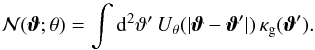 (10)We use the exponential filter function introduced by van Waerbeke (1998),
 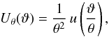 (11)with
 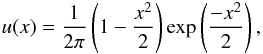 to make predictions for the third-order moments of the aperture mass and aperture number count at zero lag and with equal aperture sizes:
 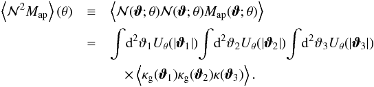 (12)For homogeneous random fields such as κ and κg, the ensemble average
  is independent of the position of the center of the aperture and can be calculated by angularly averaging the product
  . In our analysis we follow Saghiha et al. (2012) and calculate predictions for by averaging the product
  over the simulated area. Third-order aperture statistics can also be calculated from measurements of the lens-lens-shear correlator
  via integral transformations (Schneider & Watts 2005). We did this to obtain the CFHTLenS measurements.
3. Data
3.1. CFHTLenS galaxies
The multi-colour lensing survey CFHTLenS (Heymans et al. 2012; Erben et al. 2013; Miller et al. 2013), incorporates u∗g′r′i′z′ multi-band data from the CFHT Legacy Survey Wide Programme. It covers 154 deg2 of the sky and its accurate photometry has provided photometric redshifts of 7 × 10⁶ galaxies (Hildebrandt et al. 2012). The stellar masses of galaxies are estimated by fitting a model of the spectral energy distribution (SED) to the galaxy photometry. In this method, a set of synthetic SEDs are generated using a stellar population synthesis (SPS) model, and the maximum likelihood SED template that fits the observed photometry of a galaxy is obtained. Thus the SED fitting method relies on the assumptions of the SPS models, the star formation histories, the initial mass function (IMF), and the dust extinction models. The stellar masses of CFHTLenS galaxies are estimated using the SPS model of Bruzual & Charlot (2003) and assuming an IMF by Chabrier (2003). By taking into account the error on the photometric redshift estimates and the uncertainties in the SED fitting, Velander et al. (2014) estimate that the statistical uncertainties on the stellar mass estimates of CFHTLenS galaxies are about 0.3 dex.
In Simon et al. (2013), the G3L analysis of CFHTLenS data is presented in terms of aperture statistics for a sample of source galaxies with i′< 24.7 and mean redshift of z = 0.93, and lens galaxies brighter than i′< 22.5. The foreground sample is further subdivided into six stellar mass bins as given in Table 1. These stellar mass bins are then further split into two photometric redshift samples, 0.2 ≤ zph< 0.44 (“low-z”) and 0.44 ≤ zph< 0.6 (“high-z”). The redshift distribution of galaxies in these samples can be found in Fig. 5 of Simon et al. (2013). We utilize these for the predictions of the lensing statistics.
Binning by stellar mass of CFHTLenS galaxies for the low-z and high-z samples.
3.2. Mock galaxies
We use simulated lensing data that was obtained by a ray-tracing algorithm applied to the MS, which is an N-body simulation that traces the evolution of 21603 particles in a cubic region of comoving side length 500 h-1Mpc from redshift z = 127 to the present time (MS, Springel et al. 2005). The MS assumes a Λ −CDM cosmology with parameters based on 2dFGRS (Colless et al. 2001) and first-year WMAP data (Spergel et al. 2003). These parameters are summarized in Table 2.
Cosmological parameters for the assumed cosmology in the MS.
We use galaxy catalogs from B06, G11, L12, and H15 that were implemented on the MS1. All these four models use similar treatments for basic physical baryonic processes such as gas cooling, star formation, and feedback from supernovae and AGNs, but they differ in various details. We refer to some of these differences later in the paper.
The gravitational lensing in the MS is computed by using the multiple-lens-plane ray-tracing algorithm of Hilbert et al. (2009) in 64 fields-of-view of 4 × 4 deg2 each. The resulting synthetic data include the convergence and shear, on regular meshes of 40962 pixels, of sources at a set of redshifts given by the output times of the simulation snapshots. These are then combined into convergence and shear fields for the CFHTLenS redshift distribution. Furthermore, the data contain the image positions, redshifts, stellar masses, and various other galaxy properties of the galaxies computed by the SAMs. We generate mock galaxy samples that are similar to the lens samples observed in CFHTLenS by following three steps.
Firstly, we convert the SAM magnitudes to the Megacam AB magnitudes in CFHTLenS. We convert the SDSS AB magnitudes of Garching models to Megacam AB magnitude  by applying the conversion relation from Erben et al. (2013):
  (13)We convert the SDSS Vega magnitudes of Durham models to CFHTLenS AB magnitudes using2:
 ![Mathematical equation: \begin{equation} i_{\text{AB}}^{\prime} = (i_{\text{Vega}} + 0.401) - 0.085\left ( \left [r_{\text{Vega}} + 0.171\right ] - \left [i_{\text{Vega}} + 0.401 \right ] \right ). \end{equation}](/articles/aa/full_html/2017/05/aa29608-16/aa29608-16-eq80.png) (14)We then select lens galaxies brighter than
(14)We then select lens galaxies brighter than  . The redshift distribution of all flux-limited galaxies from the B06 model that fall into the stellar-mass bin sm2 is shown in Fig. 1.
Secondly, to emulate the CFHTLenS error of stellar masses, we randomly add Gaussian noise with RMS 0.3 dex to the stellar mass log M∗ in the mocks. The resulting redshift distribution of galaxies in B06 is also shown in Fig. 1.
Finally, as can be seen in Fig. 1 by comparing the dashed black curve to the red or blue curves, the redshift distribution of model galaxies differs from that of CFHTLenS. To select a realistic simulated sample, the mock samples must have the same redshift distributions as the corresponding CFHTLenS samples to produce the same lensing efficiency. Therefore, in the last step, we use a rejection method to reproduce the redshift distribution of galaxies in CFHTLenS. In this step, we randomly discard a galaxy at redshift z from the mock sample if  (15)is satisfied for a random number in the range zero to one. The distribution of selected galaxies in the low-z and high-z samples are not shown in Fig. 1 because they are practically identical to the corresponding CFHTLenS distributions.
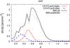 |
Fig. 1 Number density distribution per unit solid angle and redshift interval of flux-limited galaxies in sm2. The total area below each curve is the total number density of galaxies. The blue and red curves show the distribution of CFHTLenS galaxies in the low-z and high-z samples, respectively. The solid black curve represents all galaxies of the B06 model above the flux limit and with stellar mass in the sm2 bin. The dashed black curve shows the distribution when also applying a random error to the stellar masses of the B06 galaxies. |
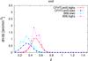 |
Fig. 2 Similar to Fig. 1, the blue and red curves show the distribution of CFHTLenS galaxies in the low-z and high-z samples, respectively. The curves labeled as “B06.lowz” (cyan) and “B06.highz” (magenta) correspond to a sample of galaxies selected from the distribution shown by the dashed black curve in Fig. 1 after adding the error of photometric redshifts in CFHTLenS to the mock redshifts. |
We note that in the method described above, we have not included the error in the photo-z estimation. However, including this kind of an uncertainty has no effect on the statistical properties of the SAM galaxy distributions. Indeed, Fig. 2 shows the true redshift distribution of B06 galaxies for low-z and high-z samples after including an emulated photo-z error, and after applying the same photo-z cuts as in CFHTLens. For this, we chose galaxies from the “B06.scattered” distribution, indicated by the dashed black curve in Fig. 1, and added a random Gaussian photo-z error with RMS 0.04(1 + z) (Hildebrandt et al. 2012). The PDF of the true redshifts of low-z and high-z samples are labeled “B06.lowz” and “B06.highz” in Fig. 2. Despite having slightly different amplitudes, these distributions have similar shapes as the “CFHTLenS.lowz” (blue) and “CFHTLenS.highz” (red) distributions, respectively. After applying the rejection method on those distributions, one obtains mock galaxy samples that have the same statistical properties of the mock galaxy samples that we produce following the three steps described previously.
4. Results
4.1. Galaxy-galaxy lensing
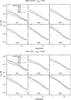 |
Fig. 3 GGL as a function of the projected separation for the six stellar mass samples according to Table 1. The top panel corresponds to the high-z sample and the bottom panel to the low-z sample. The data points with error bars, which indicate the standard error of the mean over 129 fields, show the CFHTLenS measurements, which are compared to the predictions by B06 (solid lines), G11 (dashed lines), L12 (double-dashed lines), and H15 (dashed-dotted lines). The B06 predictions for sm1 show the error of the mean over 64 fields. |
Figure 3 shows the azimuthally-averaged tangential shear ⟨γt⟩(θ) for an angular range of 0.5–35 arcmin as measured in CFHTLenS in comparison to the SAM predictions. The samples are split into stellar mass and redshift. For both CFHTLenS data and model galaxies, the amplitude of the GGL signal increases with stellar mass. For a given stellar mass bin, the amplitudes of the observed and simulated signals decrease when increasing the lens-source separation θ.
To quantify the significance of the difference between model predictions and CFHTLenS measurements of ⟨γt⟩, we compute 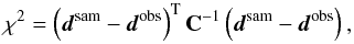 (16)where dsam and dobs are data vectors containing the SAMs predictions and CFHTLenS measurements, respectively. The covariance matrix C of the difference signal is Csam + Cobs because SAMs and CFHTLenS measurements are uncorrelated. Here Csam is the field-to-field covariance of SAMs estimated using 64 simulated fields, and Cobs is the jackknife covariance of CFHTLenS measurements using Nobs = 129 fields-of-view of 1 × 1 deg2 each. We construct Nobs jackknife samples and store the mean of the combined samples, excluding the ith field, in the data vector di. The vector d shall be the average of all di vectors. The jackknife covariance of the sample mean is then
 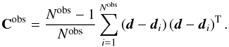 (17)For our χ2 test, we have C ≃ Cobs because the elements of the SAMs covariance matrix are negligible in comparison with the elements of the CFHTLenS covariance matrix. We apply the estimator of Hartlap et al. (2007) to obtain an estimator for the inverse of the covariance C-1 for Cobs,
 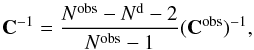 (18)when Nd<Nobs−2. The parameter Nd is the number of data points and Nobs = 129 is the number of jackknife realizations used for Cobs.
For Nd = 15 degrees of freedom, a tension between CFHTLenS and the SAM predictions with 95% confidence is given by values of χ2/ 15 > 1.67 (written in bold in Table 3). The results from Table 3 clearly show that the Durham models are in tension for all the stellar mass bins except for sm5 in the high-z sample and sm6. In comparison, the Garching models are consistent with the observations apart from possible tensions for sm3 and sm5 at low-z.
To quantify the overall difference in GGL between the SAMs and CFHTLenS, we combined the measurements of all stellar mass samples and tested for a vanishing difference signal consisting of Nd = 90 data points. Because data points between different stellar masses are correlated, we estimate a new 90 × 90 covariance by jackknifing the combined bins in 129 CFHTLenS and for the 64 mock fields. The results of the χ2 test are presented in Table 4. A tension between model and observation is now indicated by χ2/ 90 > 1.26 at the 95% confidence level. According to the χ2 test, only the predictions of H15 for the low-z sample are in agreement with the CFHTLenS. The Durham models show the strongest tension.
4.2. Galaxy-galaxy-galaxy lensing
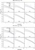 |
Fig. 4 Measurements of the G3L aperture statistics as a function of the aperture scale θ in CFHTLenS (blue symbols) and SAMs (black curves). Measurements are presented for various stellar mass and redshift, high-z and low-z, samples. Error bars indicate the standard error of the mean. The dotted vertical lines show the limits of the range used for our χ2 analysis. |
The  values measured in CFHTLenS for the low-z and high-z samples in all stellar mass bins are shown in Fig. 4. The predictions from the SAMs are also shown there. The observed
  signal is dominated by the “transformation bias” below 1 arcmin and above 10 arcmin (Simon et al. 2008). This bias is caused by galaxy blending and the finite size of the observed field, thus leading to insufficient sampling of the three-point correlation function (Kilbinger et al. 2006). Therefore, only data points between 1′<θ< 10′ are used for comparison, indicated by the dashed vertical lines in the top left panel. We retain Nd = 8 data points for each stellar mass and redshift bin.
Our measurements show that the Garching models predictions agree better with CFHTLenS than the Durham models predictions. The Durham models over-predict the signal in all but the highest stellar mass bin. In addition, the tension between Durham models and CFHTLenS is more prominent for G3L than in the GGL measurements as can be deduced from the χ2 values in Table 5. Model measurements with χ2/ 8 > 1.94 at the 95% confidence level, meaning those for which the SAM signal is inconsistent with CFHTLenS, are written in bold.
Values represent the mean satellite fraction and the mean halo mass over 64 simulated fields for the high-z and low-z samples.
Similar to GGL, we combine the G3L measurements, Nd = 48, of all stellar mass samples to quantify the overall difference between SAMs and CFHTLens. We estimate a new 48 × 48 covariance by jackknifing the combined bins in 129 CFHTLenS and for the 64 mock fields. The results of the χ2 test are presented in Table 6. A tension between model and observation is now indicated by χ2/ 48 > 1.35 at the 95% confidence level. According to the χ2 test, only the predictions of H15 for the low-z sample are in agreement with the CFHTLenS.
4.3. Stellar mass distribution
Given the foregoing results, we tested whether the stellar masses of galaxies are systematically different between the SAMs. For this purpose, we selected mock galaxies, as described in Sect. 3.2, for a broad stellar mass bin including M∗ from 5 × 10¹⁰–3.2 × 10¹¹M⊙, and plot the resulting distribution dN/ dlog M∗ in Fig. 5 for 63 bins in M∗. The number of galaxies N in a bin is normalized by the total number Ntot in the plotted range. The ratios of the model predictions and the CFHTLenS results are shown in the upper panel of each plot. For comparison, on top of the plot we indicate the labels corresponding to the stellar mass samples sm1-sm6. The SAMs results are lower than that of CFHTLenS in high stellar mass bins, and their distributions drop more quickly. In low stellar mass bins, there are differences between G11 and B06 compared to H15; for instance there is a dip for B06 in the range sm2 to sm4 compared to H15. The stellar mass distribution of H15 is the closest to CFHTLenS.
5. Discussion
In this work, we studied second- and third-order galaxy-mass correlation functions in terms of average tangential shear ⟨γt⟩ and aperture statistics  , respectively. We used mock galaxies from the Durham models B06 and L12, and the Garching models G11 and H15, which are SAMs implemented on the Millennium Simulation (MS). We compared our results with the observational results of CFHTLenS for galaxies binned in stellar mass within 0.6 <M∗/ 1010M⊙< 32 and redshift within 0.2 ≤ zph< 0.6. In addition, all lens galaxies are subject to a flux limit of .
Our results indicate that not all models can reproduce the GGL and G3L observations although there is an overall qualitative agreement between the models and CFHTLenS as visible in Figs. 3 and 4. All models best agree among each other and with CFHTLenS for sm6, meaning for stellar masses of ~2 × 10¹¹M⊙. However, the uncertainties of the CFHTLenS results are also largest here. At lower stellar masses, the Durham models clearly over-predict the amplitude of both GGL and G3L so that these models can be decisively excluded at the 95% confidence level, see Tables 3 and 5. The agreement between the Garching models and CFHTLenS, on the other hand, is good although the overall comparison to G3L still indicates some tension, see Table 6. The fit of the more recent H15 is slightly better compared to G11. We also find from our χ2 values that G3L has more discriminating power than GGL on the same data, as anticipated in Saghiha et al. (2012). This may be understood as G3L being more sensitive to the clustering amplitude of the lenses when compared to GGL. For a linear deterministic bias b of the lens number density, the G3L signal is proportional to b2 whereas the GGL signal is proportional to b.
A systematically high galaxy-matter correlation in the Durham models might indicate that the stellar masses of galaxies in these models are systematically higher compared to the Garching models. This kind of a bias could impact the matter environment, clustering, and hence GGL and G3L of stellar-mass-selected galaxies. However, this is probably not the case here for the following reason. Knebe et al. (2015) compare the stellar mass function (SMF) at z = 0 in fourteen various SAMs, including a model similar to B06 and an earlier version of H15, H13, by Henriques et al. (2013). They study whether the SMF variations could be due to the different initial mass functions (IMF) assumed in the models; B06 assumes a Kennicutt (1983) IMF whereas H15 and H13 use a Chabrier (2003) IMF. They transform the stellar masses of galaxies using Chabrier IMF, using the correction from Mitchell et al. (2013), for all the models and show that the scatter in SMF is only slightly changed by this transformation. Therefore, the specific IMFs of B06 and H15 or H13 are probably not the reason for the different lensing signals in our data. For our galaxy sample, we show the variations in the stellar mass distribution of galaxies between different SAMs (Fig. 5). We find that although both SMFs of the Durham models and G11 differ from that of H15, the GGL and G3L predictions of G11 and H15 are consistent, whereas there is a significant difference between the predictions of the Durham models and H15. This makes it unlikely that the discrepant predictions by the Durham models can be attributed to the somewhat different distribution of stellar masses.
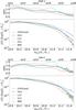 |
Fig. 5 Stellar mass function of galaxies normalized with the total number of galaxies in all three SAMs and CFHTLenS. We used a sample of sm1 to sm6 combined, and repeated the three-step selection in Sect. 3.2 to produce high-z (top) and low-z (bottom) subsamples. The top of each panel shows the ratio between the SAM and CFHTLenS stellar mass function. |
The discrepancies in model prediction of the lensing signals indicate model variations in the galaxy-matter correlations. They reflect the variations in the way galaxies are distributed among the dark matter halos. This argument is in agreement with the results presented in Kim et al. (2009) and Saghiha et al. (2012) who attributed this trend in B06 to the generation of too many satellite galaxies in massive halos. Indeed, the mean halo masses are higher in the Durham models than in the Garching models for all stellar masses but sm6 and the satellite fraction is somewhat higher for the Durham models (Table 7). One main general difference between the Durham and Garching models is the definition of independent halos and the way that descendants of the halos are identified in the merger trees. These differences have an impact on the treatment of some physical processes such as mergers which, in turn, influence the abundance of satellites in halos. Using a halo model description, Watts & Schneider (2005) show that the galaxy-matter power spectrum, and hence the GGL signal, increases in amplitude when the mean number of galaxies inside the halos of a specific mass scale is increased. Similarly, the galaxy-galaxy-matter bispectrum, hence G3L, increases in amplitude if the the number of galaxy pairs is increased for a mass scale. Therefore, an over-production of satellite galaxies in massive halos can explain the relatively high signals of GGL and G3L in the Durham models. This interpretation is supported by the higher mean mass of parent halos of galaxies in the Durham models compared to the Garching models as shown in Table 7.
One prominent improvement in H15 is that the simulations are rescaled to the Planck cosmology according to the method described in Angulo & White (2010) and Angulo & Hilbert (2015). However, here we use the H15 model adjusted to the original MS cosmology.
Acknowledgments
We thank Hendrik Hildebrandt, Douglas Applegate, and Reiko Nakajima for useful discussions. We also thank Violeta Gonzalez-Perez and the anonymous referee for fruitful comments. Hananeh Saghiha gratefully acknowledges financial support of the Deutsche Forschungsgemeinschaft through the project SI 1769/1-1. Stefan Hilbert acknowledges support by the DFG cluster of excellence “Origin and Structure of the Universe” (http://www.universe-cluster.de).
References
- Angulo, R. E., & Hilbert, S. 2015, MNRAS, 448, 364 [NASA ADS] [CrossRef] [Google Scholar]
- Angulo, R. E., & White, S. D. M. 2010, MNRAS, 405, 143 [NASA ADS] [Google Scholar]
- Angulo, R. E., Springel, V., White, S. D. M., et al. 2012, MNRAS, 426, 2046 [CrossRef] [Google Scholar]
- Bartelmann, M., & Schneider, P. 2001, Phys. Rep., 340, 291 [NASA ADS] [CrossRef] [Google Scholar]
- Baugh, C. M. 2006, Rep. Prog. Phys., 69, 3101 [NASA ADS] [CrossRef] [Google Scholar]
- Bower, R. G., Benson, A. J., Malbon, R., et al. 2006, MNRAS, 370, 645 [NASA ADS] [CrossRef] [Google Scholar]
- Brainerd, T. G., Blandford, R. D., & Smail, I. 1996, ApJ, 466, 623 [NASA ADS] [CrossRef] [Google Scholar]
- Bruzual, G., & Charlot, S. 2003, MNRAS, 344, 1000 [NASA ADS] [CrossRef] [Google Scholar]
- Chabrier, G. 2003, PASP, 115, 763 [NASA ADS] [CrossRef] [Google Scholar]
- Clampitt, J., Sánchez, C., Kwan, J., et al. 2017, MNRAS, 465, 4204 [NASA ADS] [CrossRef] [Google Scholar]
- Colless, M., Dalton, G., Maddox, S., et al. 2001, MNRAS, 328, 1039 [NASA ADS] [CrossRef] [Google Scholar]
- Erben, T., Hildebrandt, H., Miller, L., et al. 2013, MNRAS, 433, 2545 [NASA ADS] [CrossRef] [Google Scholar]
- Gladders, M. D., & Yee, H. K. C. 2005, ApJS, 157, 1 [NASA ADS] [CrossRef] [Google Scholar]
- Guo, Q., White, S., Boylan-Kolchin, M., et al. 2011, MNRAS, 413, 101 [NASA ADS] [CrossRef] [Google Scholar]
- Hartlap, J., Simon, P., & Schneider, P. 2007, A&A, 464, 399 [NASA ADS] [CrossRef] [EDP Sciences] [Google Scholar]
- Henriques, B. M. B., White, S. D. M., Thomas, P. A., et al. 2013, MNRAS, 431, 3373 [NASA ADS] [CrossRef] [Google Scholar]
- Henriques, B. M. B., White, S. D. M., Thomas, P. A., et al. 2015, MNRAS, 451, 2663 [NASA ADS] [CrossRef] [Google Scholar]
- Heymans, C., Van Waerbeke, L., Miller, L., et al. 2012, MNRAS, 427, 146 [NASA ADS] [CrossRef] [Google Scholar]
- Hilbert, S., Hartlap, J., White, S. D. M., & Schneider, P. 2009, A&A, 499, 31 [NASA ADS] [CrossRef] [EDP Sciences] [Google Scholar]
- Hildebrandt, H., Erben, T., Kuijken, K., et al. 2012, MNRAS, 421, 2355 [NASA ADS] [CrossRef] [Google Scholar]
- Hoekstra, H., van Waerbeke, L., Gladders, M. D., Mellier, Y., & Yee, H. K. C. 2002, ApJ, 577, 604 [NASA ADS] [CrossRef] [Google Scholar]
- Kauffmann, G., Colberg, J. M., Diaferio, A., & White, S. D. M. 1999, MNRAS, 303, 188 [NASA ADS] [CrossRef] [Google Scholar]
- Kennicutt, Jr., R. C. 1983, ApJ, 272, 54 [NASA ADS] [CrossRef] [EDP Sciences] [Google Scholar]
- Kilbinger, M., Schneider, P., & Eifler, T. 2006, A&A, 457, 15 [NASA ADS] [CrossRef] [EDP Sciences] [Google Scholar]
- Kim, H.-S., Baugh, C. M., Cole, S., Frenk, C. S., & Benson, A. J. 2009, MNRAS, 400, 1527 [NASA ADS] [CrossRef] [Google Scholar]
- Knebe, A., Pearce, F. R., Thomas, P. A., et al. 2015, MNRAS, 451, 4029 [NASA ADS] [CrossRef] [Google Scholar]
- Lagos, C. d. P., Bayet, E., Baugh, C. M., et al. 2012, MNRAS, 426, 2142 [NASA ADS] [CrossRef] [Google Scholar]
- Leauthaud, A., Tinker, J., Bundy, K., et al. 2012, ApJ, 744, 159 [NASA ADS] [CrossRef] [Google Scholar]
- Mandelbaum, R., Seljak, U., Kauffmann, G., Hirata, C. M., & Brinkmann, J. 2006, MNRAS, 368, 715 [Google Scholar]
- Miller, L., Heymans, C., Kitching, T. D., et al. 2013, MNRAS, 429, 2858 [Google Scholar]
- Mitchell, P. D., Lacey, C. G., Baugh, C. M., & Cole, S. 2013, MNRAS, 435, 87 [NASA ADS] [CrossRef] [Google Scholar]
- Saghiha, H., Hilbert, S., Schneider, P., & Simon, P. 2012, A&A, 547, A77 [NASA ADS] [CrossRef] [EDP Sciences] [Google Scholar]
- Schaye, J., Crain, R. A., Bower, R. G., et al. 2015, MNRAS, 446, 521 [Google Scholar]
- Schneider, P. 1996, MNRAS, 283, 837 [NASA ADS] [CrossRef] [Google Scholar]
- Schneider, P., & Watts, P. 2005, A&A, 432, 783 [NASA ADS] [CrossRef] [EDP Sciences] [Google Scholar]
- Schneider, P., Kochanek, C., & Wambsganss, J. 2006, Gravitational lensing: strong, weak and micro, Saas-Fee Advanced Course: Swiss Society for Astrophysics and Astronomy (Springer) [Google Scholar]
- Simon, P., Watts, P., Schneider, P., et al. 2008, A&A, 479, 655 [NASA ADS] [CrossRef] [EDP Sciences] [Google Scholar]
- Simon, P., Erben, T., Schneider, P., et al. 2013, MNRAS, 430, 2476 [NASA ADS] [CrossRef] [EDP Sciences] [Google Scholar]
- Spergel, D. N., Verde, L., Peiris, H. V., et al. 2003, ApJS, 148, 175 [NASA ADS] [CrossRef] [Google Scholar]
- Springel, V., White, S. D. M., Tormen, G., & Kauffmann, G. 2001, MNRAS, 328, 726 [Google Scholar]
- Springel, V., White, S. D. M., Jenkins, A., et al. 2005, Nature, 435, 629 [NASA ADS] [CrossRef] [PubMed] [Google Scholar]
- van Uitert, E., Hoekstra, H., Velander, M., et al. 2011, A&A, 534, A14 [NASA ADS] [CrossRef] [EDP Sciences] [Google Scholar]
- van Uitert, E., Cacciato, M., Hoekstra, H., et al. 2016, MNRAS, 459, 3251 [NASA ADS] [CrossRef] [Google Scholar]
- van Waerbeke, L. 1998, A&A, 334, 1 [NASA ADS] [Google Scholar]
- Velander, M., van Uitert, E., Hoekstra, H., et al. 2014, MNRAS, 437, 2111 [NASA ADS] [CrossRef] [Google Scholar]
- Viola, M., Cacciato, M., Brouwer, M., et al. 2015, MNRAS, 452, 3529 [CrossRef] [Google Scholar]
- Vogelsberger, M., Genel, S., Springel, V., et al. 2014, MNRAS, 444, 1518 [NASA ADS] [CrossRef] [Google Scholar]
- Watts, P., & Schneider, P. 2005, in Gravitational Lensing Impact on Cosmology, eds. Y. Mellier, & G. Meylan, IAU Symp., 225, 243 [Google Scholar]
- White, S. D. M., & Frenk, C. S. 1991, ApJ, 379, 52 [NASA ADS] [CrossRef] [Google Scholar]
All Tables
Values represent the mean satellite fraction and the mean halo mass over 64 simulated fields for the high-z and low-z samples.
All Figures
|
Fig. 1 Number density distribution per unit solid angle and redshift interval of flux-limited galaxies in sm2. The total area below each curve is the total number density of galaxies. The blue and red curves show the distribution of CFHTLenS galaxies in the low-z and high-z samples, respectively. The solid black curve represents all galaxies of the B06 model above the flux limit and with stellar mass in the sm2 bin. The dashed black curve shows the distribution when also applying a random error to the stellar masses of the B06 galaxies. |
| In the text | |
|
Fig. 2 Similar to Fig. 1, the blue and red curves show the distribution of CFHTLenS galaxies in the low-z and high-z samples, respectively. The curves labeled as “B06.lowz” (cyan) and “B06.highz” (magenta) correspond to a sample of galaxies selected from the distribution shown by the dashed black curve in Fig. 1 after adding the error of photometric redshifts in CFHTLenS to the mock redshifts. |
| In the text | |
|
Fig. 3 GGL as a function of the projected separation for the six stellar mass samples according to Table 1. The top panel corresponds to the high-z sample and the bottom panel to the low-z sample. The data points with error bars, which indicate the standard error of the mean over 129 fields, show the CFHTLenS measurements, which are compared to the predictions by B06 (solid lines), G11 (dashed lines), L12 (double-dashed lines), and H15 (dashed-dotted lines). The B06 predictions for sm1 show the error of the mean over 64 fields. |
| In the text | |
|
Fig. 4 Measurements of the G3L aperture statistics as a function of the aperture scale θ in CFHTLenS (blue symbols) and SAMs (black curves). Measurements are presented for various stellar mass and redshift, high-z and low-z, samples. Error bars indicate the standard error of the mean. The dotted vertical lines show the limits of the range used for our χ2 analysis. |
| In the text | |
|
Fig. 5 Stellar mass function of galaxies normalized with the total number of galaxies in all three SAMs and CFHTLenS. We used a sample of sm1 to sm6 combined, and repeated the three-step selection in Sect. 3.2 to produce high-z (top) and low-z (bottom) subsamples. The top of each panel shows the ratio between the SAM and CFHTLenS stellar mass function. |
| In the text | |
Current usage metrics show cumulative count of Article Views (full-text article views including HTML views, PDF and ePub downloads, according to the available data) and Abstracts Views on Vision4Press platform.
Data correspond to usage on the plateform after 2015. The current usage metrics is available 48-96 hours after online publication and is updated daily on week days.
Initial download of the metrics may take a while.