| Issue |
A&A
Volume 600, April 2017
|
|
|---|---|---|
| Article Number | A105 | |
| Number of page(s) | 15 | |
| Section | Interstellar and circumstellar matter | |
| DOI | https://doi.org/10.1051/0004-6361/201630285 | |
| Published online | 06 April 2017 | |
Accretion disk coronae of intermediate polar cataclysmic variables
3D magnetohydrodynamic modelling and thermal X-ray emission
1 Dip. di Fisica e Chimica, Specola Universitaria, Università degli Studi di Palermo, Piazza del Parlamento 1, 90134 Palermo, Italy
e-mail: This email address is being protected from spambots. You need JavaScript enabled to view it.
2 INAF–Osservatorio Astronomico di Palermo, Piazza del Parlamento 1, 90134 Palermo, Italy
Received: 19 December 2016
Accepted: 14 February 2017
Abstract
Context. Intermediate polar cataclysmic variables (IPCV) contain a magnetic, rotating white dwarf surrounded by a magnetically truncated accretion disk. To explain their strong flickering X-ray emission, accretion has been successfully taken into account. Nevertheless, observations suggest that accretion phenomena might not be the only process behind it. An intense flaring activity occurring on the surface of the disk may generate a corona, contribute to the thermal X-ray emission, and influence the system stability.
Aims. Our purposes are: investigating the formation of an extended corona above the accretion disk, due to an intense flaring activity occurring on the disk surface; studying the effects of flares on the disk and stellar magnetosphere; assessing its contribution to the observed thermal X-ray flux.
Methods. We have developed a 3D magnetohydrodynamic (MHD) model of a IPCV system. The model takes into account gravity, disk viscosity, thermal conduction, radiative losses, and coronal flare heating through heat injection at randomly chosen locations on the disk surface. To perform a parameter space exploration, several system conditions have been considered, with different magnetic field intensity and disk density values. From the results of the evolution of the model, we have synthesized the thermal X-ray emission.
Results. The simulations show the formation of an extended corona, linking disk and star. The flaring activity is capable of strongly influencing the disk configuration and possibly its stability, effectively deforming the magnetic field lines. Hot plasma evaporation phenomena occur in the layer immediately above the disk. The flaring activity gives rise to a thermal X-ray emission in both the [ 0.1−2.0 ] keV and the [ 2.0−10 ] keV X-ray bands.
Conclusions. An intense coronal activity occurring on the disk surface of an IPCV can affect the structure of the disk depending noticeably on the density of the disk and the magnetic field of the central object. Moreover, the synthesis of the thermal X-ray fluxes shows that this flaring activity may contribute to the observed flickering thermal X-ray emission.
Key words: novae, cataclysmic variables / stars: flare / magnetohydrodynamics (MHD) / accretion, accretion disks / stars: coronae / X-rays: stars
© ESO, 2017
1. Introduction
DQ Her stars, also known as intermediate polar cataclysmic variables (IPCVs), contain an accreting, magnetic, rapidly rotating white dwarf. The white dwarf in IPCVs typically has a magnetic field strength ranging between 0.1 and 10 MG (Hellier 2007), weaker than the field of other classes of cataclysmic variables (CVs), such as AM Her stars, also known as polar cataclysmic variables (PCVs). In particular, differently from AM Her stars, the field is not strong enough to prevent an accretion disk from forming, but it is capable of disrupting the inner part of the disk where the magnetosphere dominates the accretion. So, in IPCVs, accreting matter follows the magnetic field lines within the magnetosphere delimited by the truncation radius Rd, that is where the magnetic pressure is approximately equal to the total gas pressure.
IPCVs, with a medium-strength field, combine the characteristics of a non-magnetic system (in its outer regions) with those of a strongly magnetized object (in the region close to the white dwarf). Moreover, IPCV class stars are also strong X-ray emitters and the ratio between X-ray and visible flux (Fx/Fv) is greater than unity for this class of stars (Patterson 1994). These stars are indeed soft X-ray [ 0.1−2.0 ]keV and hard X-ray [ 2.0−10 ]keV sources with asynchronous changes of brightness. Nevertheless, while X-rays from IPCVs do exhibit aperiodic variability, this is not the most notable aspect of the X-ray timing properties of these objects. In fact, one of the defining characteristics of IPCVs is the strictly periodic and coherent X-ray spin modulation, that is, the presence of a rapid and stable periodicity in the lightcurve of the CV typically observed at optical or X-ray wavelengths with Pspin<Porb, although most stars have Pspin ≪ Porb. There is a large consensus in the literature that the origin for this X-ray emission is the mass accretion (Patterson 1994). The value of mass accretion rate Ṁ in IPCVs has been inferred from observations through various techniques based on different assumptions, and the expected value of Ṁ usually ranges between 10-11 and 10-8M⊙ yr-1 (Patterson 1984, 1994; Giovannelli et al. 2012). A significant amount of energy per particle is therefore released, due to shocks generated by the accreting plasma flowing along the field lines and impacting onto the white dwarf’s surface at, approximately, free fall velocity. According to the model of an accreting white dwarf, these impacts should cause a strong emission in the hard X-ray band [2−10keV] up to Lhx ≈ 1034ergs-1 (e.g. Patterson 1994).
Another intriguing feature shared by all the CV stars, including IPCVs, is the flickering, that is, a random, broad-band and short term modulation of luminosity. It appears as a sequence of overlapping flares and bursts apparently having no cycle or periodicity. This phenomenon has been observed in the X-ray lightcurves of CVs of all classes, and ranges from fluctuations lasting a few seconds to larger changes in brightness with rises and dips lasting for hours, with no pattern or period. The fact that flickering is a characteristic feature of all CVs immediately suggests that more than one mechanism must be involved. This is supported by the statistical properties of the flickering of the various type of CV (Bruch 2000). In fact, studies of the flickering in CV stars conducted by Fritz & Bruch (1998) suggest an origin of this phenomenon for magnetized CVs (such as IPCVs) leading to properties which are distinct from those of non-magnetic CVs. In particular, IPCVs show a strong flickering on short timescales with a high strength. Observations suggest that in some systems flickering may arise in the turbulent inner region of the disk, or from the bright spots on the surface of the white dwarf (Hellier 2001). Actually, the analysis of eclipsing lightcurves (Horne & Stiening 1985) demonstrated that the flickering source must be concentrated in the inner portion of the accretion disk but it is not necessarily confined to the immediate vicinity of the white dwarf, possibly spreading out in the inner part of the accretion disk (Bruch 2015).
The differentially rotating disk is thought to be a turbulent environment. The theoretical studies of Balbus & Hawley (1991) predicted that the turbulence in accretion disks may be driven by magneto-rotational instability (MRI) and this phenomenon has also been observed through numerical models (e.g. Hawley 1991; Stone et al. 1996). This may lead to magnetic reconnection phenomena. Regarding this, we should note that significant parts of the disk can be turbulent, therefore, reconnection is possible at different distances from the star. On the other hand, the studies of Galeev et al. (1979) showed that the differential rotation of the Keplerian disk is able to lead to the winding of the magnetic field lines, increasing the field and determining the phenomenon of the expulsion of the magnetic field from the disk in the form of loops. Through the magnetic energy release, due to magnetic reconnection, an extended magnetic corona can be built up and sustained (Beloborodov 1999; Malzac et al. 2001). Similar phenomenon has been observed in simulations of MRI disks, where the magnetic corona has been formed and expanded above and below the disk due to winding of the field lines and amplification of the magnetic field (Armitage 2002; Steinacker & Papaloizou 2002). The formation of an extended corona has also been observed in simulations of accretion onto magnetized stars from an MRI-driven disk (Romanova et al. 2011). Hence, the combination of a turbulent disk and its differential rotation may trigger an exponential amplification of a seed magnetic field (Beloborodov 1999; Galeev et al. 1979). The resulting magnetic field is sufficiently strong to cause magnetic reconnection close to the disk surface where the observations suggest that phenomena responsible for flickering may occur (Hellier 2001; Seward & Charles 2010).
In the light of these considerations, it is plausible that the X-ray emission observed in some of the IPCV stars may have a thermal component due to a flaring activity occurring on the surface of the accretion disk. This flaring activity is to some extent similar to the flares taking place in the corona of the Sun and solar-like stars, and may develop and sustain an extended corona.
It is worth noting that in the models cited above, the presence of the stellar magnetic field is not required for the formation of an extended corona in the disk; in fact, high-energy X-ray coronae are also observed in objects, where the stellar magnetic field is not present (e.g. black holes). In particular for CVs, there are no remarkable differences in the properties of extended coronae observed from magnetic (such as IPCVs) and non-magnetic CVs, since the main features differentiating these two types of CV are: the presence of circular polarization of the emission due to the interaction of accreting charged material with magnetic field; a spin period lower than orbital period Pspin ≪ Porb; HeII emission lines due to ionization of the accretion columns by the extreme ultraviolet (EUV) continuum of the radial accretion shock (Szkody et al. 2003); and the properties of flickering (Fritz & Bruch 1998), whose origin may be mainly related to accretion, that in magnetized objects is thought to occur via accretion columns or curtains (Romanova et al. 2002, 2003).
Here we perform 3D magnetohydrodynamic (MHD) simulations of the formation of accretion disk coronae in different prototypes of IPCVs through a hail of flares occurring on the surface of the disk. The flares are stocastically triggered injecting energy into the system by means of a heat pulse with random intensity. We consider a magnetized central object with different intensities of the magnetic field. Although this is not a requirement for the formation of the corona, in this way we may reproduce the formation of coronal loops linking star and disk. Similar structures have been predicted using MHD models (Orlando et al. 2011) and observed in young stellar objects (Favata et al. 2005).
2. Model and numerical setup
The model describes an intense flaring activity taking place on the surface of the accretion disk placed around a rotating magnetized compact object, a prototype of IPCV. The central compact object is surrounded by a structured atmosphere initially unperturbed and approximately in equilibrium. In order to study IPCVs, we adapted the model described in Orlando et al. (2011) developed for classical T-Tauri stars (CTTS).
2.1. MHD equations
The system evolution can be described through the four time-dependent classical MHD equations, extended to include gravitational force, viscosity, thermal conduction, radiative cooling, and plasma heating. These equations are defined in a 3D spherical coordinate system (r, θ, φ) and they are here reported in c.g.s. in the conservative form: 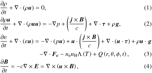 where p is the thermal pressure for a fully ionized plasma, and the total energy per unit volume (ε) is the sum of internal or thermal (εi) and kinetic energy (Ek), with γ = 5/3:
 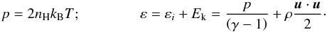 (5)The mass density is defined as ρ = μmHnH, where mH is the mass of hydrogen atom, nH is the number of hydrogen atoms per unit of volume, and μ = 1.28 (assuming metal abundances of 1, equal to solar ones) is the mean atomic mass (Anders & Grevesse 1989). The bulk velocity of the plasma is defined as u. Moreover, Eq. (4) has been taken into account in the ideal limit of high magnetic Reynolds number (Rm ≫ 1).
The viscosity is taken into account in MHD equations through the viscous tensor τ. The viscosity is assumed to be effective only in the circumstellar disk and negligible in the region of the extended corona (Orlando et al. 2011; Giovannelli et al. 2012). The technique used to track the disk material, where viscosity is effective, is based on the definition of a tracer following the same evolution of density (i.e. the tracer is passively advected similarly to the density). We defined the tracer Cd as the disk mass fraction inside each computational cell, initializing the disk material with Cd = 1 and the extended corona with Cd = 0. Then the viscosity is enabled only in the computational cells containing at least 99% of material of the disk (i.e. Cd> 0.99). The viscous stress tensor is defined as: ![Mathematical equation: \begin{equation} \vec{\tau} = \eta_{\rm v}\left[ \left( \nabla \vec{u} \right) + \left( \nabla \vec{u} \right)^{\rm T} - \frac{2}{3} \left( \nabla \cdot \vec{u} \right) \vec{I} \right], \label{eq:ViscTensor} \end{equation}](/articles/aa/full_html/2017/04/aa30285-16/aa30285-16-eq34.png) (6)where dynamic (or shear) viscosity ηv is proportional to kinematic viscosity νv and density as follows:
(6)where dynamic (or shear) viscosity ηv is proportional to kinematic viscosity νv and density as follows: 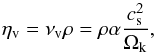 (7)where
  is the isothermal sound speed and Ωk is the angular velocity of the circumstellar disk in quasi-Keplerian rotation. In Eq. (7), α is a phenomenological dimensionless parameter defined in the Shakura & Sunyaev model taking into account the effect of anomalous viscosity (Shakura & Sunyaev 1973). In this model, α can be assumed to be a measure of the strength of the turbulent angular momentum transport and varies in the range 0.01−0.6 (Balbus 2003). In the simulations here presented, we assumed constant α = 0.02 (Romanova et al. 2002).
Thermal conduction appears in the energy Eq. (3) as minus the heat flux divergence (− ∇·Fc). In accordance with the standard formulation by Spitzer (Spitzer 1962), thermal conduction is highly anisotropic due to the presence of the magnetic field that drastically reduces the conductivity component transverse to the field. As a matter of fact, thermal flux can be locally split into two components, one along and the other across the magnetic field lines:  (8)The two components of thermal flux can therefore be written as
 ![Mathematical equation: \begin{eqnarray} \begin{split} &F_{\parallel} = \left[ q_{\rm spi} \right]_{\parallel} = -k_{\parallel} \left( \nabla_{\parallel}T \right) \approx -9.2 \times 10^{-7} T^{\frac{5}{2}} \left( \nabla_{\parallel}T \right) \\ &F_{\perp} = \left[ q_{\rm spi} \right]_{\perp} = -k_{\perp} \left( \nabla_{\perp}T \right) \approx -3.3 \times 10^{-16} \frac{n_{\rm H}^{2}}{T^{\frac{1}{2}}B^{2}} \left( \nabla_{\perp}T \right), \label{eq:ThermCond_q_spi} \end{split} \end{eqnarray}](/articles/aa/full_html/2017/04/aa30285-16/aa30285-16-eq45.png) (9)where k∥ and k⊥ are the thermal conduction coefficients along and across field lines (in units of erg s-1 K-1 cm-1). From Eq. (9) it is clear that, if the magnetic field is sufficiently strong, the ratio k⊥/k∥ ≪ 1 and thermal conduction behaves anisotropically working prevalently along field lines. Moreover, the classical theory of thermal conduction is based on the assumption that the mean free path λ is smaller than the temperature scale height LT, and when the requirement
(9)where k∥ and k⊥ are the thermal conduction coefficients along and across field lines (in units of erg s-1 K-1 cm-1). From Eq. (9) it is clear that, if the magnetic field is sufficiently strong, the ratio k⊥/k∥ ≪ 1 and thermal conduction behaves anisotropically working prevalently along field lines. Moreover, the classical theory of thermal conduction is based on the assumption that the mean free path λ is smaller than the temperature scale height LT, and when the requirement 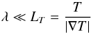 (10)is not fullfilled, Eq. (8) overestimates thermal flux. When fast phenomena occur, like flares in their early phases, it is well known that rapid transients, fast dynamics, and steep gradients develop (Reale & Orlando 2008). So, under these circumstances, Spitzer’s heat conduction formulation breaks down becoming flux limited, and therefore cannot be suitable (Brown et al. 1979). For this reason the two components of thermal conduction must be redefined as follows (Orlando et al. 2008):
 ![Mathematical equation: \begin{eqnarray} \begin{split} &F_{\parallel} = \left( \frac{1}{\left[ q_{\rm spi} \right]_{\parallel}} + \frac{1}{\left[ q_{\rm sat} \right]_{\parallel}} \right)^{-1} \\ &F_{\perp} = \left( \frac{1}{\left[ q_{\rm spi} \right]_{\perp}} + \frac{1}{\left[ q_{\rm sat} \right]_{\perp}} \right)^{-1}, \label{eq:ThermCond_F_spi_sat} \end{split} \end{eqnarray}](/articles/aa/full_html/2017/04/aa30285-16/aa30285-16-eq52.png) (11)where the saturated heat flux along and across field lines are (Cowie & McKee 1977)
(11)where the saturated heat flux along and across field lines are (Cowie & McKee 1977) ![Mathematical equation: \begin{eqnarray} \begin{split} &\left[ q_{\rm sat} \right]_{\parallel} = -\textrm{sign} \left( \nabla_{\parallel}T \right) \cdot 5\varphi\rho c_{\rm s}^{3} \\ &\left[ q_{\rm sat} \right]_{\perp} = -\textrm{sign} \left( \nabla_{\perp}T \right) \cdot 5\varphi\rho c_{\rm s}^{3}. \label{eq:ThermCond_q_sat} \end{split} \end{eqnarray}](/articles/aa/full_html/2017/04/aa30285-16/aa30285-16-eq53.png) (12)In Eq. (12), ϕ is a parameter we set equal to unity (Giuliani 1984; Borkowski et al. 1989; Fadeyev et al. 2002).
(12)In Eq. (12), ϕ is a parameter we set equal to unity (Giuliani 1984; Borkowski et al. 1989; Fadeyev et al. 2002).
The calculation were performed using PLUTO (Mignone et al. 2007), a modular Godunov-type code developed mainly for astrophysical plasmas involving high Mach number flows in multiple spatial dimensions. The code embeds different physics modules (allowing the treatment of hydrodynamics and magneto-hydrodynamics both relativistic and non-relativistic in Cartesian or curvilinear coordinates) and multiple algorithms particularly oriented toward the treatment of astrophysical flows in the presence of discontinuities. These features make PLUTO a flexible and versatile modular computational framework to solve the equations describing astrophysical plasma flows. PLUTO is entirely written in the C programming language and was designed to make efficient use of massive parallel computers using the message-passing interface (MPI) library for interprocessor communications. The MHD equations are solved using the available MHD module, configured to compute inter-cell fluxes with the Harten-Lax-Van Leer (HLL) approximate Riemann solver. In order to solve the equation versus time, we used a second order Runge-Kutta (RK) integration scheme. Moreover, a minmod limiter for the primitive variables has been used, in order to avoid spurious oscillations that could otherwise occur due to shocks, discontinuities, or sharp changes in the solution domain. As for magnetic field, its evolution is computed adopting the constrained transport approach (Balsara & Spicer 1999) that maintains the solenoidal condition (∇·B = 0) at machine accuracy. Moreover, we adopted the magnetic field-splitting technique (Tanaka 1994; Powell et al. 1999; Zanni & Ferreira 2009) by splitting the total magnetic field into a contribution coming from the background stellar magnetic field and a perturbation to this initial field. Then only the latter component is computed numerically. This approach is particularly useful when dealing with low-β plasma as is the case in the proximity of the stellar surface (Zanni & Ferreira 2009). PLUTO takes into account radiative losses from optically thin plasma. The radiative losses are computed as 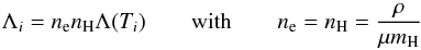 (13)at the temperature of interest, using a lookup-table and interpolation method1, where Λi = Λ(Ti) is available along with Ti as a sampling at a discrete point (see Fig. 1). The thermal conduction as well the viscosity is treated separately from advection terms through operator splitting. In particular we adopted the super-time-stepping technique (Alexiades et al. 1996) which has been proved to be very effective to speed up explicit time-stepping schemes for parabolic problems. This approach is crucial when high values of plasma temperature are reached (as during flares), the explicit scheme being subject to a rather restrictive stability condition (i.e. Δt< (Δx)2/ (2η), where η is the maximum diffusion coefficient), as the thermal conduction timescale τcond is typically shorter than the dynamical one τdyn (Hujeirat & Camenzind 2000; Hujeirat 2005; Orlando et al. 2005, 2008).
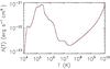 |
Fig. 1 Radiative losses per unit emission measure Λ(T) as a function of temperature. |
2.2. Initial and boundary conditions: barotropic stellar atmosphere
Most IPCVs have a 0.8−0.9 M⊙ white dwarf for which an appropriate radius is R∗ = 6.0 × 108 cm (i.e. 10-2R⊙). Nevertheless, being aware of this, we deliberately decided to consider a star more massive, with a mass at the limit of its class. This choice has been made in order to have a more rapidly evolving system, due to higher orbital velocity, thus reducing computational costs. After all, the mass of the central compact object has no other effect on the qualitative evolution of the system. For these reasons, we located a compact object of mass M∗ ≃ 1.4 M⊙ and spin period of 5.4 min (Patterson 1994; Norton et al. 1999; Putney 1999) at the origin of a 3D spherical coordinate system.
The magnetic field of the white dwarf is supposed to be in a force-free dipole-like initial configuration (Hellier 2007), with the magnetic dipole aligned with the rotation axis of the star. The dipolar magnetic field may be decomposed into two components in spherical coordinate as follows: 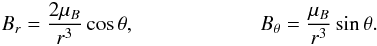 (14)The magnetic moment μB has been chosen so as to get the desired magnetic field intensity at the stellar surface Bsup, ranging between 1.5 × 10⁵ G and 107 G in the several configurations explored (see Table 1). The magnetosphere is defined as a quasi-cylindrical region of radius equal to the truncation radius Rd where the disk structure begins in the equatorial plane. This region, surrounding the central star, is assumed to rotate as a rigid body with the same angular velocity as the star (ω∗ = ωmag) (see Figs. 2a and 3b).
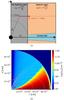 |
Fig. 2 a) Scheme of the cross section of the differentially rotating domain regions and definition of some physical quantities; b) colour-coded log scale of density distribution in the computational domain used in the preliminary 2.5D simulation. White lines represent projected magnetic field lines, whilst the magenta line (marked by arrows) is the β = 1 surface (run F4f1.00a). |
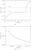 |
Fig. 3 Distribution of some physical quantities: a) density profile along a spherical surface for fixed radius (R = 1.7 × 1011 cm) and for θ between 0° (rotation axis) and 90° (equatorial plane), the horizontal dashed lines show the density of the disk (ρd) and the corona (ρc) at the contact layer; b) angular velocity of the disk in the equatorial plane, the vertical dashed line identifies the truncation radius (Rd) (run F4f1.00a). |
The accretion disk in our model consists of relatively cold (Td ≈ 5 × 10⁴ K) isothermal plasma rotating with angular velocity close to the Keplerian value (Orlando et al. 2011). Disk density is structured in order to follow the barotropic prescription (see below) and has been chosen in order to get an inner disk particle density nd ranging between ≈1010 cm-3 and ≈1014 cm-3 in the various system configurations considered (see Table 1). The disk is initially truncated by the stellar magnetosphere at the truncation radius Rd, where there is equilibrium between plasma and magnetic pressure and therefore the ratio of the plasma pressure to the magnetic pressure, β = 8π(p + ρv2) /B2, is close to unity. In accordance with the other parameters chosen, Rd has been placed at 2.7 × 1010 cm from the centre of the star (Hellier 1993). The co-rotation radius, where plasma rotates at the same angular velocity as the star, is imposed to be identical to the truncation radius, that is Rcor = Rd. This assumption is based on the belief that most intermediate polars are in a sort of rotational equilibrium (Warner 1996; Norton et al. 1999). Basically, the accretion disk is disrupted at the radius (Rd) where the Keplerian rotation of the disk is equal to that of the white dwarf, that is ω∗ = ωd(Rd).
The extended corona is a shell of optically thin and hot gas above the accretion disk (Giovannelli et al. 2012). In our model this region has a density following the barotropic prescription (see below), whilst temperature is imposed to be initially uniform and equal to Tcor = 107 K, defining an isothermal low density region extending above the surface of the disk and connecting it with the central star.
In order to define a circumstellar medium in a quiescent configuration, we adopted the barotropic conditions introduced by Romanova et al. (2002). These initial conditions satisfy mechanical equilibrium involving centrifugal, gravitational, and pressure gradient forces. Generalizing hydrostatic balance equation, we can consider different contributions to the force, beyond the gravitational one:  (15)The various contributions to the ℱ function are gravitational (φg), centrifugal (φc), and a non-Keplerian correction (φKep). They are defined as follows:
 ![Mathematical equation: % subequation 2057 0 \begin{eqnarray} &&\phi_{\rm Kep}=\left(k-1\right) \frac{GM_{*}}{R_{\rm d}};\\[10pt] &&\phi_{\rm g} =\frac{GM_{*}}{r};\\[10pt] &&\phi_{\rm c} = \begin{cases} -\int_{\infty}^{R_{\rm d}}\omega_{\rm d}^{2}r\ {\rm d}r &\!\!\!\!-\int_{R_{\rm d}}^{r}\omega_{\rm m}^{2}r\ {\rm d}r =\\& k\frac{GM_{*}}{R_{\rm d}}\left[ 1 + \frac{R_{\rm d}^2-r^{2}}{2R_{\rm d}^2} \right] \qquad (r\leq R_{\rm d}) \\ \\ -\int_{\infty}^{r}\omega_{\rm d}^{2}r\ {\rm d}r &\!\!\!\!\!= k\frac{GM_{*}}{r} \qquad\qquad\qquad\;\; (r\geq R_{\rm d}). \end{cases} \label{eq:Potentials} \end{eqnarray}](/articles/aa/full_html/2017/04/aa30285-16/aa30285-16-eq130.png) Here, r = Rsinθ is the cylindrical radius and k = 1.01 is a parameter taking into account that the disk is slightly non-Keplerian. Moreover, (see Figs. 2a and 3b) the angular velocity of the plasma is given by
Here, r = Rsinθ is the cylindrical radius and k = 1.01 is a parameter taking into account that the disk is slightly non-Keplerian. Moreover, (see Figs. 2a and 3b) the angular velocity of the plasma is given by 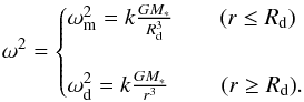 (17)In Eq. (17) we distinguish ωm, the angular velocity of the magnetosphere, where plasma is rotating as a rigid body, from ωd, the angular velocity of the quasi-Keplerian region. Using the perfect gas law
  , we can compute the pressure at the contact layer between the corona and disk:
 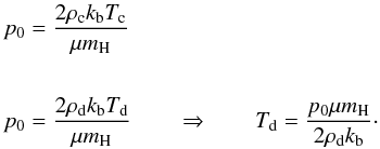 (18)Here we take as input parameters coronal temperature (Tc), coronal density (ρc), and disk density (ρd), for which the ratio ρd/ρc = 200 at disk surface (see Table 1). Finally, Eq. (15) yields pressure as a function of ℱ
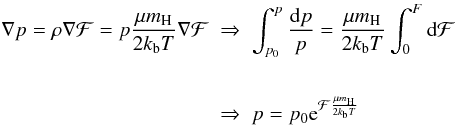 (19)and finally we get pressure and density as follows
 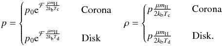 (20)From these values we obtain an analytic function describing density and pressure with the whole domain taken into account (see Figs. 2b and 3a).
It is important to note that barotropic initial conditions provide a smooth start-up for the evolution of the system and, in particular, of the magnetic field, threading the disk and the corona. In fact, the corona above the disk rotates with the same angular velocity as the disk, and there is no contact discontinuity which is expected otherwise, if the corona were not rotating (Romanova et al. 2002, 2003).
Barotropic initial conditions along with a dipole-like magnetic field configuration may be considered an useful analytic description of a quasi equilibrium system. Nevertheless, due to the interaction with the disk, where β> 1 and plasma dynamics dominate, the magnetic field is strongly influenced by the Keplerian rotation of the disk. Consequently, after a certain amount of time, the magnetic field is expected to be deformed and put into a coil shape due to the interaction with the disk. In order to get a configuration of the system as realistic as possible, we divided the numerical simulations into two distinct steps.
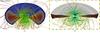 |
Fig. 4 Result of the simulation performed to generate the initial configuration of the 3D simulation: a) cutaway view of the simulations after ~2.5 h with a fully developed magnetic field. The yellow box contains the region mapped in 3D and used as the initial condition of the 3D simulations; b) rendering of the initial condition of 3D simulations, the borders of the figure are the same as those of the yellow box in the left panel (run F3f1.00c). |
As a first step, we ran several 2.5D simulations with a square computational domain of 114 × 64 cells in spherical coordinates  and initial conditions defined by Eqs. (15)–(20). The radial direction has been discretized on a grid with space steps increasing exponentially with R. The domain extends from Rmin ≈ 9 × 109 cm to Rmax ≈ 1.8 × 1012 cm. With this choice, the inner boundary does not coincide with the stellar surface and, therefore, the region closer to the star is not taken into account in our simulations. We made this choice for two main reasons: first, this region does not have a relevant impact on our study, which is rather focused on the evolution of the region above the disk surface; second, in this way we avoid computational cells having very small δθ mesh size, because they dramatically increase the computational time. The radial grid is made of nr = 114 points with a maximum resolution of ΔR = 4.2 × 108 cm, close to the star, and ΔR = 8.2 × 1010 cm, at the external end of the domain. The disk has been externally truncated at R = 9 × 1011 cm, that is, approximately at half radial domain. The boundary conditions at Rmin (i.e. at the end close to the star) are assumed so that infalling material follows field lines, passing through the surface of the boundary as an outflow (Romanova et al. 2002). At Rmax, a zero-gradient boundary condition is assumed. As for the angular coordinate θ, it ranges from 0° (rotation axis) to 90° (equatorial plane) and has been discretized uniformly using nθ = 64 points, giving a resolution of Δθ ~ 1.4°. For θ = 0° (i.e. rotation axis), axisymmetric boundary conditions are assumed; that is, we prescribe a sign change across the boundary of all vectorial components, except for components along the axis itself. For θ = 90° (i.e. equatorial plane), equatorial-symmetric boundary conditions are assumed; that is, we prescribe a sign change across the boundary of the normal component of velocity and of the component of the magnetic field tangential to the interface. We let the magnetic field interact with the disk for almost 2.5h of physical time so as to reach an almost steady state configuration. It is worth noting that, in this preliminary step of the implemented two-phase technique, the whole size of the domain and disk has been intentionally overestimated in order to avoid undesired boundary effects during the evolution of the system. In fact, several tests showed that the prescription of a zero-gradient boundary condition (i.e. an “outflow b. c.”) at the outer end of the disk might not reproduce correctly the dynamics of the plasma, resulting in an underestimate of the plasma inflow. To this end, in the following phase we take into account only the inner part of the 2.5D domain (see Fig. 4).
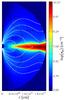 |
Fig. 5 Colour-coded log scale of density distribution in a slice of the computational domain used as initial condition in the 3D simulation (see Fig. 4b). White lines represent the magnetic field lines projected in the [ r,θ ] plane, whilst the black line is the β = 1 surface with the β< 1 region on the left (run F3f1.00c). |
As a second phase, we then use such a virtually relaxed and steady state as the initial conditions for our project. To this end we map the output of the 2.5D MHD simulations (namely the fully developed physical quantities: mass density, temperature, velocity, and magnetic field), performed in the first phase, onto a 3D domain in order to provide the initial condition of a 3D model describing the further evolution of the star-disk system (see Fig. 4). Due to the fact that the 2.5D domain covers only a slice of half hemisphere of the system, the 2.5D-into-3D mapping has been performed through a preliminary reflection across the equatorial plane followed by a rigid rotation about the z axis. We note that the 2.5D domain has been selected in order to describe in 3D only the inner part of the whole 2.5D domain, where flaring activity is expected to occur, thus reducing the computational cost. Moreover, no phenomena relevant for the present study involve the external region of the disk. In the initial configuration of the 3D simulations (see Figs. 4b and 5) the magnetic field lines appear still in a dipole-like form. This is particularly evident in the corona closer to the star (i.e. the magnetosphere), where β< 1 and the region is field-dominated. On the other hand, in the external corona and, especially, inside the disk, where β> 1, the dynamics are matter-dominated and the differential rotation of the plasma induces a noticeable deformation of the field lines. The 3D computational domain obtained in this way is defined in spherical coordinates (r,θ,φ) and consists of a computational cube of 1283 cells. The radial direction has been discretized on a grid with interval size exponentially increasing with R. The domain extends from Rmin ≈ 9 × 109 cm to Rmax ≈ 1.8 × 1011 cm. The radial grid is made of nr = 128 points with a maximum resolution of ΔR = 2.1 × 108 cm, close to the star, and ΔR = 4.2 × 109 cm, close to the external part of the disk. The boundary conditions at Rmin and Rmax are the same as those used in the 2.5D runs. As for the angular coordinate θ, the computational domain spans an angle from ~7° to ~173°, leaving two cones above the star poles as not modelled. Hence, the boundaries in θ do not coincide with the rotational axis of the star-disk system in order to avoid extremely small δφ values which cause a strongly increasing computational cost. On the other hand, the modelling of the whole computational domain, including the two cones above the star poles, has been performed in the studies of the magnetospheric accretion onto the surface of the star (Romanova et al. 2003, 2004; Kulkarni & Romanova 2013). Moreover, all events relevant for the present study do not involve any region close to the rotation axis. In fact, in our problem we concentrate on the disk-magnetosphere interaction and heating of the inner disk. The angular coordinate θ has been discretized uniformly using nθ = 128 points, giving a resolution of Δθ ~ 1.3°. Zero-gradient boundary conditions are assumed for θ at ~7° and ~173°. Finally, in the angular coordinate φ, the computational domain spans the angle from ~0° to ~180°, with an uniform resolution of Δφ ~ 1.4°. Thus the computational domain covers only half of the star-disk system. The boundary conditions for the coordinate φ are assumed to be periodic.
2.3. Coronal heating and flaring activity
The coronal heating has been prescribed as a phenomenological term, composed of two components. The first one works at temperature T ≤ 2 × 10⁴ K and balances exactly the local radiative losses. Nevertheless, several tests on the 3D simulations showed that increasing this value to T ≤ 1MK determines a much more stable calculation and significant reduction of computational costs, with comparable results in terms of the dynamics of the plasma and X-ray emission.
The second component is transient and consists of flares occurring on the surface of the disk. Every single flare is simulated and triggered injecting energy into the system through a heat pulse. We considered the release of several flares with a randomly generated timing in order to achieve a frequency ranging from approximately one flare every 2.5 s to one flare every 100 s (Tamburini et al. 2009). The location of every heat pulse is randomly chosen in an angular interval δθ ≈ 3° reckoned from the accretion disk surface. The area subject to flaring activity is the annular region between 5.4 × 1010 cm and 1.3 × 1011 cm. This assumption stems from an observation concerning the measurement of the size of accretion disk coronae, based on ingress and egress timing, in another but similar context (Church & Bałucińska-Church 2004). The 3D spatial distribution of each pulse is defined to be Gaussian with a width of σ = 5 × 108 cm. The total time duration of every pulse is set at 100 s, afterwards the pulse is completely switched off. The time evolution of pulse intensity is divided into three equally spaced parts: a linearly increasing ramp, a steady part, and a linearly decreasing ramp. The energy is injected with a maximum intensity of H0 = 2 × 10⁵ erg cm-3 s-1. This value of power per unit volume yields a maximum total energy of a single flare of Efmax ≈ 1034 erg. As a conservative choice, we have taken values typical of large solar flares (Priest 2014). Nevertheless, the effective intensity of flares has been randomly generated with a power law with α = −2.1 (Priest 2014), approximating the intensity distribution of flares on the Sun.
2.4. Synthesis of the thermal X-ray emission
From the model results we synthesize the thermal X-ray emission originating from the disk-corona system in different spectral bands of interest: [ 0.1−2.0 ]keV and [ 2.0−10 ]keV. We apply a method analogous to the one described by Orlando et al. (2009). The results of numerical simulations are the evolution of the various physical quantities of interest (density, temperature, velocity, and magnetic field) of the plasma in half of the spatial domain. In order to get the total emitted radiation, we reconstruct the 3D spatial distribution of these physical quantities in the whole spatial domain. We rotate the system around the x axis to explore different inclinations of the orbital plane relative to the sky plane. From the value of temperature and emission measure of the ith computational cell we synthesize the corresponding thermal X-ray emission, using the astrophysical plasma emission code (APEC; Smith et al. 2001) of hot collisionally ionized plasma. APEC models provide emissivity tables of both line and continuum emission which may be used to calculate predicted fluxes. These predicted fluxes may, in turn, be compared with observed spectral features. The predicted flux is given by: 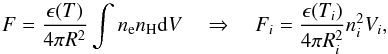 (21)where ϵ(T) is the emissivity in ergcm3/s, R is the distance to the source in cm, and the integral is the emission measure in cm-3. Therefore, defining i as the index of a cell of the computational domain, ϵ(Ti) is the emissivity of the cell at temperature Ti, whilst the emission measure is defined as
  , where ni is the proton number density in the cell and Vi is the volume of the cell where plasma is assumed to be fully ionized. The spectral synthesis takes into account the Doppler shift of emission lines due to the plasma velocity component along the line of sight (LoS). We assume the solar metal abundances of Anders & Grevesse (1989) for the circumstellar medium (CSM). The X-ray spectrum emitted by each computational cell is filtered through the CSM absorption column, going from the cell to the observer along the LoS. The CSM absorption is computed using the absorption cross-section as a function of wavelength from Balucinska-Church & McCammon (1992). The thermal X-ray emission, integrated along the LoS in the whole computational domain, defines an image describing the distribution of the thermal X-ray flux; the flux values are computed assuming a distance of 500 pc and no interstellar absorption. Then, through the integration of the fluxes of the images, we obtain the total emission at the selected time; the sequence of all these values at different times yields the lightcurve in the selected energy bands.
3. Results
The model described in Sect. 2 allows us to explore different configurations of the system, changing some main input parameters. In fact, once we set the truncation radius at Rd, where the β of plasma is imposed equal to unity, we can change the value of density at the surface of the disk and, consequently, obtain the surface magnetic field of the white dwarf needed to keep β = 1 at the truncation radius Rd. The various configurations of the system taken into account have been chosen in order to have a sampling as wide as possible of magnetic field strength found in this kind of system, that ranges between 0.1 and 10MG. We take as a reference model the one defined as F4f1.00a in Table 1, in which the surface magnetic field intensity is ≈5MG. Other parameters have been taken into account in our exploration of the parameter space. In particular we explored the maximum intensity of the flares and their frequency as well. Table 1 summarizes the various simulations and details the main parameters characteristic of each run: ρc and ρd are, respectively, coronal density and disk density at the layer between corona and disk; Tc is the initial uniform temperature of the corona; nd is the maximum density of particles in the bulk of the disk; Bsup is the magnetic field intensity at the surface of the star; FF is the frequency of flare release, and finally Imax is the maximum energy release of the flares.
3.1. System dynamics
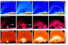 |
Fig. 6 Two following flaring loops during their evolution. The figure shows the distribution of density (upper panels), pressure (middle panels), and temperature (lower panels) in a slice in the [ r,θ ] plane passing through the middle of the loops. In the upper panels white lines represent magnetic field lines projected in the [ r,θ ] plane, while the black line shows the β = 1 surface. The slice encompasses an angular sector going from the rotation axis to the disk equatorial plane. The first flare occurs in a β> 1 region, surrounded with β< 1 region, and produces a magnetically confined loop linking star and disk. The second flare is also released in a β> 1 region, but at a larger distance from the star and at approximately the same angle φ, compared with the first flare. It appears a bit later in time, at time t = 93 s, and becomes bright at t = 155 s. Differently from the first flare, the hot plasma of the second flare is not magnetically confined (run F4f1.00a). |
For our reference case, F4f1.00a, the energy release of the intense flaring activity was followed for approximately 20 min. Each heat pulse is injected into the system through the parametric term Q(r,θ,φ,t) in Eq. (3) at randomly chosen locations on both the upper and lower surfaces of the disk, and triggers a MHD shock wave that develops above the disk, preferentially propagating away from the central star, in the region where β> 1. The abrupt release of energy determines a local increase of temperature and pressure, heating the dense plasma of the disk. While each flare develops, the heat pulse determines an overpressure in the region of the disk corresponding to the footpoint of the loop2. This overpressure travels as a pressure wave through the bulk of the disk, eventually reaching the opposite surface of the disk. The heated disk material expands in the magnetosphere propagating above the disk with a strong evaporation front moving at a speed of the order of 108 cm/s. The heated and expanding plasma interacts with the magnetic field, with mutual effects. As a matter of fact, during the evolution of the system, the field lines, in regions where β has high values, are dragged away and slowly deformed by the action of the flares, and, eventually, only the magnetosphere close to the star keeps an approximately dipolar shape. Analogously, the hot evaporation front triggered by each flare is strongly affected by the interaction with the magnetosphere, and, where β< 1, the hot plasma is channelled along the magnetic field lines toward the central white dwarf. A few minutes after each energy release, a hot (T ~ 109 K) magnetic loop of length of the order of 1010 cm is formed, linking the disk with the star. The loop continues to expand for almost eight minutes, and the temperature decreases by almost two orders of magnitude. The frames in Fig. 6 show the evolution of density, pressure and temperature distribution of two successive flares in a slice of the domain perpendicular to the equatorial plane and aligned with the symmetry axis. The first flare occurs in a low β region closer to the star, whereas the second one occurs in a high β region. Both flares are triggered at approximately the same angle φ. For the first flare, the magnetic field, due to a low β, produces the channelling of the hot plasma, forming a magnetic loop linking the star and disk, while the second one appears as not magnetically confined. The plasma starts cooling as soon as the heat deposition is over, as a result of the combined action of the efficient radiative cooling and thermal conduction. In particular, on one hand, thermal conduction from the outer layer of hot plasma sustains the disk evaporation that goes on even after the flare decays. On the other hand, thermal conduction, due to its high anisotropy in the presence of the magnetic field (see Eq. (9)), promotes the development of a hot magnetic tube (loop) linking star and disk, through the formation of a fast thermal front propagating along the magnetic field lines toward the star and reaching it in a timescale of ≈1min (lower panels of Fig. 6).
 |
Fig. 7 Effect of a hail of flares on the disk and on the circumstellar atmosphere. The cutaway views of the star-disk system show the mass density (blue) and the magnetic field lines (green) at different times. The 3D volume rendering of the plasma temperature is over-plotted, showing the flaring loops (red-yellow) linking the inner part of the disk with the central white dwarf (run F4f1.00a). |
 |
Fig. 8 Different effects of the same energy release at the same time (t = 311.50s) on different configurations of the system with progressively denser disks and stronger magnetic field, from top to bottom. The cutaway views of the star-disk system show the mass density (blue) and the magnetic field lines (green). The 3D volume rendering of the plasma temperature is over-plotted, showing the flaring loops (red-yellow). |
In Fig. 7 a 3D rendering of the evolution of the system is represented. During the system evolution, the combined effect of the storm of flares causes the formation of an extended corona between disk and star (see panels in Fig. 7). Nevertheless, most of the evaporated disk material, particularly in the external regions of the disk, is not completely confined by the magnetic field and is not efficiently channelled into the loops but it escapes upward and is ejected away into the outer regions, carrying away mass and angular momentum.
The main difference between the various models explored lies in the density of the circumstellar atmosphere and in the magnetic field intensity. It is worth noting that β must be always greater than unity inside the disk. This implies that, for example, in a low density disk the magnetic field intensity is correspondingly low, and the energy release during the reconnection process is also smaller. Therefore, a low-density disk could not be capable of generating strong flares. With an analogous reasoning, the reverse occurs in high density configurations. For this reason, in all the configurations explored we have always taken into account values of magnetic field intensity and disk density to keep β> 1 inside the disk. Keeping this crucial caution in mind, we explored disks with different densities, however, we kept the maximum energy released by flares the same, in order to obtain comparable simulations of the various configurations taken into account. Due mainly to a denser disk, the effects of the pressure wave moving across the disk caused by each flare are mild in configurations with a denser disk and a stronger magnetic field (i.e. runs F4f1.00a and F5f1.00a, see bottom panels in Fig. 8). In these two cases, the perturbation of the disk is limited to the surface of the disk and the field lines are slowly deformed by the action of the MHD shock. On the other hand, the flares cause a perturbation that is more evident in low density and weak field configurations (i.e. runs F3f1.00c and F6f1.00a, see top panels in Fig. 8). Moreover, in these configurations, the perturbation of the disk causes a fast and evident deformation of the field lines. So, due to a less dense disk, the flaring activity can strongly alter the configuration of the disk, potentially hampering its overall stability.
Another important element differentiating the various models is how often and how intense is the energy release associated to each flare. As expected, frequency and intensity of the flares have remarkable effects on the disk and on the magnetic field lines. In fact, a higher flare frequency or a more intense energy release produces a noticeable disk disruption along with a deeper dislocation of the magnetic field lines, compared to analogous models characterized by a less intense and less frequent flaring activity.
It is worth noting that we have simulated an intense flaring activity through randomly parametrized heat releases, thus flares do not develop as a result of the dynamics of the system, although their presence is justified by the magnetic interaction in a turbulent and differentially rotating disk. In our model, the seed magnetic field in the disk is due to the presence of a magnetized white dwarf. However, as mentioned in Sect. 1, a magnetized central object is not required for the formation of an extended disk corona. In the presence of a non-magnetized central object, we expect that loops may form as a consequence of the phenomenon of the expulsion of the magnetic field from the disk (Galeev et al. 1979), therefore linking different regions of the disk. We conclude, therefore, that the only significant difference between the cases explored here and those considering a non-magnetized central object is the presence of magnetic loops linking the disk to the star, as observed in our simulations.
3.2. Thermal X-ray emission
Since we are interested in investigating the thermal X-ray emission originating from the activity occurring on the surface of the disk, finally, we analyzed the emission measure (see Sect. 2.4) of the plasma at a temperature capable of producing thermal X-ray emission (T> 106 K). Figure 9 shows that, immediately after the beginning of the release of heat pulses, the amount of plasma at a temperature greater than 1MK, increases steadily reaching an almost steady-state condition after 100 s. The values of emission measure found indicate that the flaring activity leads to a strong thermal X-ray emission.
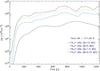 |
Fig. 9 Total emission measure vs. time of plasma hotter than 1 MK. After a few minutes, the value of emission measure approaches a virtually steady-state condition (run F4f1.00a). |
From the model results, we synthesized the thermal X-ray emission originating from the whole system along the whole interval of time considered in our simulations. The method applied is described in Sect. 2.4. The X-ray emission has been synthesized in two bands: the soft ([ 0.1−2.0 ]keV) and the hard ([ 2.0−10 ]keV). Figure 10 shows some of the synthesized X-ray images. Each image shows the simulated spatial distribution of X-ray flux observed at different times during the evolution of the system. The system is observed from a line of sight forming a 45° angle with the equatorial plane. From these X-ray images we can infer where the coronal emission is more conspicuous. We identify the feet of the coronal loops as the regions where the X-ray emission is concentrated. On the whole, the flaring activity seems to be capable of triggering the formation of a hot and tenuous layer of plasma extending on the disk surface. This layer is accountable for the bulk of the coronal X-ray emission, that is concentrated in the proximity of the disk surface.
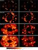 |
Fig. 10 X-ray images of the whole domain as seen by an observer with a line of sight of 45° with the equatorial plane. On the left column panels are soft X-ray [ 0.1−2.0 ]keV flux values, on the right hand side panels, hard X-ray [ 2.0−10 ]keV flux values. The flux values are computed assuming a distance of 500 pc and no interstellar absorption. The images refer to run F4f1.00a and are taken at the same times as those of Fig. 7. |
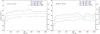 |
Fig. 11 Comparative plot of lightcurves relative to various configurations explored for different values of magnetic field. On the left panel, soft X-ray band [ 0.1−2.0 ]keV lightcurves; on the right panel, hard X-ray band [ 2.0−10 ]keV lightcurves. |
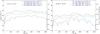 |
Fig. 12 Comparative plot of lightcurves relative to the reference model. The explored parameter is the frequency of the energy pulse (flares). On the left panel, soft X-ray band [ 0.1−2.0 ]keV lightcurves; on the right panel, hard X-ray band [ 2.0−10 ]keV lightcurves. |
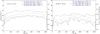 |
Fig. 13 Comparative plot of lightcurves relative to the reference model. The explored parameters are the frequency and the intensity of the energy pulse (flares). On the left panel, soft X-ray band [ 0.1−2.0 ]keV lightcurves; on the right panel, hard X-ray band [ 2.0−10 ]keV lightcurves. |
The flux values of the thermal X-ray emission have been used in order to obtain the lightcurves for each model. The flux is defined as the total energy per unit of surface and per unit of time and the corresponding luminosity is obtained from the flux values supposed to be measured at a distance of 500 pc. Figure 11 shows the comparison between the lightcurves of the various configurations studied imposing a frequency of a flare every five seconds (assumed as reference value). The luminosity, in every configuration explored, reaches in a few minutes the quasi-stationary condition and exhibits a clear oscillation. This effect is actually less noticeable in low field configurations (i.e. runs F3f1.00c and F6f1.00a) because these configurations are characterized by low density values. The density, through the term nenH (see Eq. (3)), strongly affects the radiative cooling. So, in low density configurations, the energy injected by each heat pulse is more slowly dissipated than in high density ones, and, when another pulse is released, the effect of the energy injected by the previous one has not been dissipated yet. In this case the effect of each flare is less evident in the global light curve.
Another key element, that we can infer from the lightcurves, is the maximum luminosity achieved: the denser the disk (and, consequently, given the way our model is devised, the stronger the magnetic field), the higher the luminosity. In fact, a denser plasma determines a higher value of emission measure, hence the contribution to the emission is greater. Comparing the lightcurves of the harder band with the corresponding ones of the softer band, we find a hardness ratio of the spectra, namely the ratio between hard and soft X-ray luminosity, approximately ≲0.1.
In the context of the reference model, we also explored the effect of the frequency and intensity of flares on the lightcurves. Figure 12 shows how the lightcurves are affected by different flare release frequencies. The difference between maximum and mean value ranges between a factor of five and eight of the mean value in high flare frequency configurations (run F4f1.00f, F4f1.00a and F4f10.00e), whilst, in low flare frequency ones (run F4f1.00g and F4f10.00g), this value rises up to 57 times the mean value. From this comparison, we can infer that the variability of X-ray emission strongly depends on the rate of triggered flares. Actually, as long as the period between two subsequent flares is shorter than the duration of each energy pulse (100 s), the variability of the luminosity value is less noticeable and the effect of each single flare is mixed and superimposed on the ones of the other neighbouring flares. We actually observe a background emission due to many small flares evolving simultaneously while higher peaks are due to the strongest flares. When the period between flares is the same as the duration of the energy pulse, the effect of each single pulse is easily identifiable. We can observe the fast rise and the subsequent slow decay of the thermal X-ray emission characteristic of each flare. Indeed, for high temperature plasma the conductive and the radiative cooling are more effective (see Fig. 1), causing a quicker decrease of emission. This feature determines a noticeable modulation of luminosity as a sequence of partially overlapping bursts. Furthermore, the variability of the luminosity is generally more evident in the hard than in the soft band, because the hotter plasma is the dominant source of the hard emission.
Figure 13 shows a comparison between lightcurves, taken in the context of the reference model with the same flare frequency but different maximum intensity. This comparison shows that the X-ray variability strongly depends on the flare frequency, while the main effect of a higher intensity of flares is to bring up the average luminosity keeping, at the same time, the modulated shape almost unchanged.
Finally, we note that modulation in X-ray, UV, and Vis lightcurves may be observed in IPCVs, due to the formation of a lighthouse beam, when the white dwarf’s spin and magnetic axes are not aligned, and the star magnetic field rotates with a tilted axis. This is due to the energy release of shocks generated by the accreting material impacting onto the star’s surface, creating an intense bright spot at one or both of the white dwarf’s magnetic poles. Hence, pulsations and additional periods can emerge when the rotating searchlight illuminates the various structures in the binary (e.g. Patterson 1994; Romanova et al. 2003; Kulkarni & Romanova 2008; Giovannelli et al. 2012; Romanova et al. 2013). Nevertheless, no pulsation of the coronal radiation has been observed so far (e.g. Venter & Meintjes 2007). In our work, the seed magnetic field in the disk is due to the presence of a magnetized central object. In particular we adopted the simplest magnetosphere configuration: a non-tilted dipole. Hence, our model cannot reproduce any rotational modulation of the coronal radiation. Although the search for a possible pulsation of the coronal radiation is out of the scope of the present paper, we note that the lack of observed modulation may be closely related to the fact that flares are not dependent on the large-scale configuration of the magnetic field (in fact the formation of an extended corona does not require a central magnetized object) and strongly depend on the local magnetic field configuration in the disk.
4. Conclusions
We investigated the effect of an intense flaring activity occurring on the surface of the accretion disk of various IPCV prototypes. The prototypes taken into account consider different values of density and magnetic field. We focused on different aspects: the formation of an extended corona above the disk; the contribution of the related coronal activity to the thermal X-ray emission from these objects; the conditions able to jeopardize the stability of the disk.
We have developed a 3D MHD model taking into account all the key physical processes: viscosity of the disk, magnetic-field-oriented thermal conduction, radiative cooling, and gravitational forces. In order to set up the initial conditions of the 3D simulations, we devised a two-step technique. As a first step, we ran 2.5D simulations in order to obtain a developed configuration of the magnetic field. From this we reconstructed a 3D initial condition where we then simulated a hail of flares distributed stochastically on the surface of the inner part of the accretion disk. Finally, we synthesized the thermal X-ray emission from each system all along the whole evolution.
In the light of our findings, we can draw the following main conclusions: (a) an intense flaring activity close to the surface of the accretion disk can build up an extended corona linking the star to the disk along the magnetic field lines; (b) the thermal X-ray emission from the corona is mainly emitted from a thin layer immediately above the surface of the disk; (c) the thermal X-ray luminosity due to the flaring activity may contribute to the emission observed from these objects; (d) this coronal activity can influence the disk configuration and its stability, effectively deforming the magnetic field lines, with effects strongly dependent on density and magnetic field intensity; (e) the radiative and conductive cooling has a crucial role in the modulation of luminosity due to the chain of flares, and it has a different impact on the lightcurves depending on the X-ray band considered and on the temperature of the emitting plasma, contributing efficaciously to the phenomenon of flickering originating from the inner region of the disk.
It is worth noting that the synthesized thermal X-ray emission exhibits luminosity values ranging between 1030 and 1032erg/s. These values, especially those for the high density configurations explored, are in general agreement with previous studies (Patterson et al. 1980; van der Woerd 1987; Eracleous et al. 1991; Choi et al. 1999; Venter & Meintjes 2007).
To summarize, the results presented above suggest that an intense flaring activity occurring on the surface of the accretion disk of IPCV stars may turn out to have an important effect on the structure of the system and its stability, and a key role in the formation of an extended corona, whose effects may contribute to the thermal X-ray emission observed from these objects.
The lookup table used was generated with Cloudy 90.01 for an optically thin plasma and solar abundances, thanks to T. Plewa.
The footpoint of a magnetic loop is the region at which tubes of magnetic field lines reach the surface of the disk to form coronal loops.
Acknowledgments
We wish to thank the anonymous referee for criticisms and helpful suggestions which have improved the paper. This work was supported in part by the Italian Ministry of University and Research (MIUR) and by Istituto Nazionale di Astrofisica (INAF). PLUTO is developed at the Turin Astronomical Observatory in collaboration with the Department of Physics of Turin University. We acknowledge also the CINECA Award HP10CSHHKL and the HPC facility (SCAN) of the INAF–Osservatorio Astronomico di Palermo, for the availability of high performance computing resources and support.
References
- Alexiades, V., Amiez, G., & Gremaud, P.-A. 1996, Communications in Numerical Methods in Engineering, 12, 31 [CrossRef] [Google Scholar]
- Anders, E., & Grevesse, N. 1989, Geochim. Cosmochim. Acta, 53, 197 [Google Scholar]
- Armitage, P. J. 2002, MNRAS, 330, 895 [NASA ADS] [CrossRef] [Google Scholar]
- Balbus, S. A. 2003, ARA&A, 41, 555 [NASA ADS] [CrossRef] [Google Scholar]
- Balbus, S. A., & Hawley, J. F. 1991, ApJ, 376, 214 [NASA ADS] [CrossRef] [Google Scholar]
- Balsara, D. S., & Spicer, D. S. 1999, J. Comput. Phys., 149, 270 [Google Scholar]
- Balucinska-Church, M., & McCammon, D. 1992, ApJ, 400, 699 [NASA ADS] [CrossRef] [Google Scholar]
- Beloborodov, A. M. 1999, ApJ, 510, L123 [NASA ADS] [CrossRef] [Google Scholar]
- Borkowski, K. J., Shull, J. M., & McKee, C. F. 1989, ApJ, 336, 979 [NASA ADS] [CrossRef] [Google Scholar]
- Brown, J. C., Spicer, D. S., & Melrose, D. B. 1979, ApJ, 228, 592 [NASA ADS] [CrossRef] [Google Scholar]
- Bruch, A. 2000, A&A, 359, 998 [NASA ADS] [Google Scholar]
- Bruch, A. 2015, A&A, 579, A50 [NASA ADS] [CrossRef] [EDP Sciences] [Google Scholar]
- Choi, C.-S., Dotani, T., & Agrawal, P. C. 1999, ApJ, 525, 399 [NASA ADS] [CrossRef] [Google Scholar]
- Church, M. J., & Bałucińska-Church, M. 2004, MNRAS, 348, 955 [NASA ADS] [CrossRef] [Google Scholar]
- Cowie, L. L., & McKee, C. F. 1977, ApJ, 211, 135 [NASA ADS] [CrossRef] [Google Scholar]
- Eracleous, M., Halpern, J., & Patterson, J. 1991, ApJ, 382, 290 [NASA ADS] [CrossRef] [Google Scholar]
- Fadeyev, Y. A., Le Coroller, H., & Gillet, D. 2002, A&A, 392, 735 [NASA ADS] [CrossRef] [EDP Sciences] [Google Scholar]
- Favata, F., Flaccomio, E., Reale, F., et al. 2005, ApJS, 160, 469 [NASA ADS] [CrossRef] [Google Scholar]
- Fritz, T., & Bruch, A. 1998, A&A, 332, 586 [NASA ADS] [Google Scholar]
- Galeev, A. A., Rosner, R., & Vaiana, G. S. 1979, ApJ, 229, 318 [NASA ADS] [CrossRef] [Google Scholar]
- Giovannelli, F., Sabau-Graziati, L., & VOID, V. 2012, Mem. Soc. Astron. It., 83, 446 [NASA ADS] [Google Scholar]
- Giuliani, Jr., J. L. 1984, ApJ, 277, 605 [NASA ADS] [CrossRef] [Google Scholar]
- Hawley, J. F. 1991, ApJ, 381, 496 [NASA ADS] [CrossRef] [Google Scholar]
- Hellier, C. 1993, PASP, 105, 966 [NASA ADS] [CrossRef] [Google Scholar]
- Hellier, C. 2001, Cataclysmic variable stars, Springer Praxis Books/Space Exploration (Springer) [Google Scholar]
- Hellier, C. 2007, in Star-Disk Interaction in Young Stars, eds. J. Bouvier, & I. Appenzeller, IAU Symp., 243, 325 [Google Scholar]
- Horne, K., & Stiening, R. F. 1985, MNRAS, 216, 933 [NASA ADS] [Google Scholar]
- Hujeirat, A. 2005, Comput. Phys. Commun., 168, 1 [NASA ADS] [CrossRef] [Google Scholar]
- Hujeirat, A., & Camenzind, M. 2000, A&A, 362, L41 [NASA ADS] [Google Scholar]
- Kulkarni, A. K., & Romanova, M. M. 2008, MNRAS, 386, 673 [NASA ADS] [CrossRef] [Google Scholar]
- Kulkarni, A. K., & Romanova, M. M. 2013, MNRAS, 433, 3048 [NASA ADS] [CrossRef] [Google Scholar]
- Malzac, J., Beloborodov, A. M., & Poutanen, J. 2001, MNRAS, 326, 417 [NASA ADS] [CrossRef] [Google Scholar]
- Mignone, A., Bodo, G., Massaglia, S., et al. 2007, ApJS, 170, 228 [Google Scholar]
- Norton, A. J., Beardmore, A. P., Allan, A., & Hellier, C. 1999, A&A, 347, 203 [NASA ADS] [Google Scholar]
- Orlando, S., Peres, G., Reale, F., et al. 2005, A&A, 444, 505 [NASA ADS] [CrossRef] [EDP Sciences] [Google Scholar]
- Orlando, S., Bocchino, F., Reale, F., Peres, G., & Pagano, P. 2008, ApJ, 678, 274 [NASA ADS] [CrossRef] [Google Scholar]
- Orlando, S., Drake, J. J., & Laming, J. M. 2009, A&A, 493, 1049 [NASA ADS] [CrossRef] [EDP Sciences] [Google Scholar]
- Orlando, S., Reale, F., Peres, G., & Mignone, A. 2011, MNRAS, 415, 3380 [NASA ADS] [CrossRef] [Google Scholar]
- Patterson, J. 1984, ApJS, 54, 443 [NASA ADS] [CrossRef] [Google Scholar]
- Patterson, J. 1994, PASP, 106, 209 [NASA ADS] [CrossRef] [Google Scholar]
- Patterson, J., Branch, D., Chincarini, G., & Robinson, E. L. 1980, ApJ, 240, L133 [NASA ADS] [CrossRef] [Google Scholar]
- Powell, K. G., Roe, P. L., Linde, T. J., Gombosi, T. I., & Zeeuw, D. L. D. 1999, J. Comput. Phys., 154, 284 [NASA ADS] [CrossRef] [Google Scholar]
- Priest, E. 2014, Magnetohydrodynamics of the Sun (Cambridge, UK: Cambridge University Press) [Google Scholar]
- Putney, A. 1999, in 11th European Workshop on White Dwarfs, eds. S.-E. Solheim, & E. G. Meistas, ASP Conf. Ser., 169, 195 [Google Scholar]
- Reale, F., & Orlando, S. 2008, ApJ, 684, 715 [NASA ADS] [CrossRef] [Google Scholar]
- Romanova, M. M., Ustyugova, G. V., Koldoba, A. V., & Lovelace, R. V. E. 2002, ApJ, 578, 420 [NASA ADS] [CrossRef] [Google Scholar]
- Romanova, M. M., Ustyugova, G. V., Koldoba, A. V., Wick, J. V., & Lovelace, R. V. E. 2003, ApJ, 595, 1009 [NASA ADS] [CrossRef] [Google Scholar]
- Romanova, M. M., Ustyugova, G. V., Koldoba, A. V., & Lovelace, R. V. E. 2004, ApJ, 610, 920 [NASA ADS] [CrossRef] [Google Scholar]
- Romanova, M. M., Ustyugova, G. V., Koldoba, A. V., & Lovelace, R. V. E. 2011, MNRAS, 416, 416 [NASA ADS] [Google Scholar]
- Romanova, M. M., Ustyugova, G. V., Koldoba, A. V., & Lovelace, R. V. E. 2013, MNRAS, 430, 699 [NASA ADS] [CrossRef] [Google Scholar]
- Seward, F. D., & Charles, P. A. 2010, Exploring the X-ray Universe (Cambridge University Press) [Google Scholar]
- Shakura, N. I., & Sunyaev, R. A. 1973, A&A, 24, 337 [NASA ADS] [Google Scholar]
- Smith, R. K., Brickhouse, N. S., Liedahl, D. A., & Raymond, J. C. 2001, ApJ, 556, L91 [NASA ADS] [CrossRef] [Google Scholar]
- Spitzer, L. 1962, Physics of Fully Ionized Gases (Interscience Publishers) [Google Scholar]
- Steinacker, A., & Papaloizou, J. C. B. 2002, ApJ, 571, 413 [NASA ADS] [CrossRef] [Google Scholar]
- Stone, J. M., Hawley, J. F., Gammie, C. F., & Balbus, S. A. 1996, ApJ, 463, 656 [NASA ADS] [CrossRef] [Google Scholar]
- Szkody, P., Fraser, O., Silvestri, N., et al. 2003, AJ, 126, 1499 [NASA ADS] [CrossRef] [Google Scholar]
- Tamburini, F., de Martino, D., & Bianchini, A. 2009, A&A, 502, 1 [NASA ADS] [CrossRef] [EDP Sciences] [Google Scholar]
- Tanaka, T. 1994, 111, 381 [Google Scholar]
- van der Woerd, H. 1987, Ap&SS, 130, 225 [NASA ADS] [CrossRef] [Google Scholar]
- Venter, L. A., & Meintjes, P. J. 2007, MNRAS, 378, 681 [NASA ADS] [CrossRef] [Google Scholar]
- Warner, B. 1996, Ap&SS, 241, 263 [Google Scholar]
- Zanni, C., & Ferreira, J. 2009, A&A, 508, 1117 [NASA ADS] [CrossRef] [EDP Sciences] [Google Scholar]
All Tables
All Figures
|
Fig. 1 Radiative losses per unit emission measure Λ(T) as a function of temperature. |
| In the text | |
|
Fig. 2 a) Scheme of the cross section of the differentially rotating domain regions and definition of some physical quantities; b) colour-coded log scale of density distribution in the computational domain used in the preliminary 2.5D simulation. White lines represent projected magnetic field lines, whilst the magenta line (marked by arrows) is the β = 1 surface (run F4f1.00a). |
| In the text | |
|
Fig. 3 Distribution of some physical quantities: a) density profile along a spherical surface for fixed radius (R = 1.7 × 1011 cm) and for θ between 0° (rotation axis) and 90° (equatorial plane), the horizontal dashed lines show the density of the disk (ρd) and the corona (ρc) at the contact layer; b) angular velocity of the disk in the equatorial plane, the vertical dashed line identifies the truncation radius (Rd) (run F4f1.00a). |
| In the text | |
|
Fig. 4 Result of the simulation performed to generate the initial configuration of the 3D simulation: a) cutaway view of the simulations after ~2.5 h with a fully developed magnetic field. The yellow box contains the region mapped in 3D and used as the initial condition of the 3D simulations; b) rendering of the initial condition of 3D simulations, the borders of the figure are the same as those of the yellow box in the left panel (run F3f1.00c). |
| In the text | |
|
Fig. 5 Colour-coded log scale of density distribution in a slice of the computational domain used as initial condition in the 3D simulation (see Fig. 4b). White lines represent the magnetic field lines projected in the [ r,θ ] plane, whilst the black line is the β = 1 surface with the β< 1 region on the left (run F3f1.00c). |
| In the text | |
|
Fig. 6 Two following flaring loops during their evolution. The figure shows the distribution of density (upper panels), pressure (middle panels), and temperature (lower panels) in a slice in the [ r,θ ] plane passing through the middle of the loops. In the upper panels white lines represent magnetic field lines projected in the [ r,θ ] plane, while the black line shows the β = 1 surface. The slice encompasses an angular sector going from the rotation axis to the disk equatorial plane. The first flare occurs in a β> 1 region, surrounded with β< 1 region, and produces a magnetically confined loop linking star and disk. The second flare is also released in a β> 1 region, but at a larger distance from the star and at approximately the same angle φ, compared with the first flare. It appears a bit later in time, at time t = 93 s, and becomes bright at t = 155 s. Differently from the first flare, the hot plasma of the second flare is not magnetically confined (run F4f1.00a). |
| In the text | |
|
Fig. 7 Effect of a hail of flares on the disk and on the circumstellar atmosphere. The cutaway views of the star-disk system show the mass density (blue) and the magnetic field lines (green) at different times. The 3D volume rendering of the plasma temperature is over-plotted, showing the flaring loops (red-yellow) linking the inner part of the disk with the central white dwarf (run F4f1.00a). |
| In the text | |
|
Fig. 8 Different effects of the same energy release at the same time (t = 311.50s) on different configurations of the system with progressively denser disks and stronger magnetic field, from top to bottom. The cutaway views of the star-disk system show the mass density (blue) and the magnetic field lines (green). The 3D volume rendering of the plasma temperature is over-plotted, showing the flaring loops (red-yellow). |
| In the text | |
|
Fig. 9 Total emission measure vs. time of plasma hotter than 1 MK. After a few minutes, the value of emission measure approaches a virtually steady-state condition (run F4f1.00a). |
| In the text | |
|
Fig. 10 X-ray images of the whole domain as seen by an observer with a line of sight of 45° with the equatorial plane. On the left column panels are soft X-ray [ 0.1−2.0 ]keV flux values, on the right hand side panels, hard X-ray [ 2.0−10 ]keV flux values. The flux values are computed assuming a distance of 500 pc and no interstellar absorption. The images refer to run F4f1.00a and are taken at the same times as those of Fig. 7. |
| In the text | |
|
Fig. 11 Comparative plot of lightcurves relative to various configurations explored for different values of magnetic field. On the left panel, soft X-ray band [ 0.1−2.0 ]keV lightcurves; on the right panel, hard X-ray band [ 2.0−10 ]keV lightcurves. |
| In the text | |
|
Fig. 12 Comparative plot of lightcurves relative to the reference model. The explored parameter is the frequency of the energy pulse (flares). On the left panel, soft X-ray band [ 0.1−2.0 ]keV lightcurves; on the right panel, hard X-ray band [ 2.0−10 ]keV lightcurves. |
| In the text | |
|
Fig. 13 Comparative plot of lightcurves relative to the reference model. The explored parameters are the frequency and the intensity of the energy pulse (flares). On the left panel, soft X-ray band [ 0.1−2.0 ]keV lightcurves; on the right panel, hard X-ray band [ 2.0−10 ]keV lightcurves. |
| In the text | |
Current usage metrics show cumulative count of Article Views (full-text article views including HTML views, PDF and ePub downloads, according to the available data) and Abstracts Views on Vision4Press platform.
Data correspond to usage on the plateform after 2015. The current usage metrics is available 48-96 hours after online publication and is updated daily on week days.
Initial download of the metrics may take a while.