| Issue |
A&A
Volume 600, April 2017
|
|
|---|---|---|
| Article Number | A118 | |
| Number of page(s) | 13 | |
| Section | Galactic structure, stellar clusters and populations | |
| DOI | https://doi.org/10.1051/0004-6361/201630004 | |
| Published online | 12 April 2017 | |
Chemical characterisation of the globular cluster NGC 5634 associated to the Sagittarius dwarf spheroidal galaxy⋆,⋆⋆
1 INAF–Osservatorio Astronomico di Bologna, via Ranzani 1, 40127 Bologna, Italy
e-mail: This email address is being protected from spambots. You need JavaScript enabled to view it.
2 INAF-Osservatorio Astronomico di Padova, Vicolo dell’Osservatorio 5, 35122 Padova, Italy
3 Department of Physics and Astronomy, Macquarie University, Sydney, NSW 2109, Australia
4 Monash Centre for Astrophysics, School of Physics and Astronomy, Monash University, Melbourne, VIC 3800, Australia
5 Dipartimento di Fisica e Astronomia, Università di Bologna, viale Berti Pichat 6, 40127 Bologna, Italy
6 Department of Astronomy and McDonald Observatory, The University of Texas, Austin, TX 78712, USA
Received: 3 November 2016
Accepted: 4 January 2017
Abstract
As part of our on-going project on the homogeneous chemical characterisation of multiple stellar populations in globular clusters (GCs), we studied NGC 5634, associated to the Sagittarius dwarf spheroidal galaxy, using high-resolution spectroscopy of red giant stars collected with VLT/FLAMES. We present here the radial velocity distribution of the 45 observed stars, 43 of which are cluster members, the detailed chemical abundance of 22 species for the seven stars observed with UVES-FLAMES, and the abundance of six elements for stars observed with GIRAFFE. On our homogeneous UVES metallicity scale, we derived a low-metallicity [Fe/H] =−1.867 ± 0.019 ± 0.065 dex (±statistical ±systematic error) with σ = 0.050 dex (7 stars). We found the normal anticorrelations between light elements (Na and O, Mg and Al), a signature of multiple populations typical of massive and old GCs. We confirm the associations of NGC 5634 to the Sgr dSph, from which the cluster was lost a few Gyr ago, on the basis of its velocity and position, and the abundance ratios of α and neutron capture elements.
Key words: stars: abundances / stars: atmospheres / stars: Population II / globular clusters: general / globular clusters: individual: NGC 5634
Based on observations collected at ESO telescopes under programme 093.B-0583.
Table 2 is only available at the CDS via anonymous ftp to cdsarc.u-strasbg.fr (130.79.128.5) or via http://cdsarc.u-strasbg.fr/viz-bin/qcat?J/A+A/600/A118
© ESO, 2017
1. Introduction
Once considered good examples of simple stellar populations, Galactic globular clusters (GCs) are currently thought to have formed in a complex chain of events, which left a fossil record in their chemical composition (see the review by Gratton et al. 2012). Our homogeneous FLAMES survey of more than 25 GCs (see updated references in Carretta 2015; and Bragaglia et al. 2015) combined with literature data, demonstrated that most, or perhaps all, GCs host multiple stellar populations that can be traced by the anti-correlated variations of Na and O abundances discovered by the Lick-Texas group (as reviewed by Kraft 1994; and Sneden 2000). Photometrically, GCs exhibit spread, split and even multiple sequences, especially when the right combination of filters is used. These variations can be explained in large part by different chemical compositions among cluster stars, in particular of light elements such as He, C, N and O (e.g. Sbordone et al. 2011; Milone et al. 2012).
Our large and homogeneous database allowed us, for the first time, to quantitatively study the Na-O anti-correlation. In all the analysed GCs, we found approximately one third of stars of primordial composition, similar to that of field stars of similar metallicity (only showing a trace of type II Supernovae nucleosynthesis, i.e. low Na and high O). According to the most widely accepted paradigm of GC formation (e.g. D’Ercole et al. 2008), these stars are believed to be the long-lived part of the first generation (FG) of stars formed in the cluster. The other two thirds have a modified composition (increased Na, depleted O) and belong to the second generation (SG) of stars, polluted by the most massive stars of the FG (Gratton et al. 2001) with ejecta from H burning at high temperature (Denisenkov & Denisenkova 1989; Langer et al. 1993). Unfortunately, the identification of the FG stars that produced the gas of modified composition is still unknown; we refer to Ventura et al. (2001), Decressin et al. (2007), de Mink et al. (2009), Maccarone & Zureck (2012), Denissenkov & Hartwick (2014), and Bastian et al. (2015) for example.
We found that the extension of the Na-O anticorrelation tends to be larger for higher-mass GCs and that, apparently, there is an observed minimum cluster mass for appearance of the Na-O anticorrelation (Carretta et al. 2010a). This is another important constraint for cluster-formation mechanisms because it indicates the mass at which we expect that a cluster is able to retain part of the ejecta of the FG and hence show the Na-O signature (the masses of the original clusters are expected to be much higher than the present ones, since the SG has to be formed by the ejecta of only part of the FG). It is important to understand if this limit is real or is due to the small statistics (fewer low-mass clusters have been studied, and only a few stars in each were observed). After studying the high-mass clusters, we begun a systematic study of low-mass GCs and high-mass and old open clusters (OCs) to empirically find the mass limit for the appearance of the Na-O anticorrelation and to understand if there are differences between high-mass and low-mass cluster properties, for example in the relative fraction of FG and SG stars (Bragaglia et al. 2012, 2014; Carretta et al. 2014a).
For a better understanding of multiple stellar populations in GCs, it is also fundamental to study clusters in other galaxies, a challenging task. While a promising approach seems to use abundance-sensitive colour indexes (see Larsen et al. 2014, for GCs in Fornax), only a few GCs (in Fornax and in the Magellanic Clouds) have their abundances derived using high-resolution spectroscopy (of course this does not include the known clusters associated with the Sgr dSph and now physically within the Milky Way). These GCs also seem to host two populations (Letarte et al. 2006, for Fornax; Johnson et al. 2006; and Mucciarelli et al. 2009, for old GCs in LMC) but the fractions of FG and SG stars in Fornax and LMC GCs seem to be different with respect to clusters of similar mass in the Milky Way (MW). Whether this is again a problem of low statistics or the galactic environment (a dwarf spheroidal and a dwarf irregular vs. a large spiral) influencing the GC formation mechanism remains to be seen.
To gain a deeper insight into this problem, we also included in our sample GCs commonly associated to the disrupting Sagittarius dwarf spheroidal to understand if there is a significant difference amongst GCs formed in different environments (the MW and dwarf galaxies). In fact, GCs born in a dSph may have retained a larger fraction of their original mass. After the very massive GCs, M54 (Carretta et al. 2010b) and NGC4590 (M 68: Carretta et al. 2009a,b; although this latter is not universally accepted as a member of the Sgr family), another Sgr GC of our project is Terzan 8. In this cluster we see some indication of a SG, at variance with other low-mass Sgr GCs (Ter7, Sbordone et al. 2007; Pal12, Cohen 2004). However, the SG seems to represent a small minority, contrary to what happens for high-mass GCs (Carretta et al. 2014a). In the present paper we focus on the chemical characterisation of NGC 5634, a poorly studied cluster considered to be associated to the Sgr dSph (Bellazzini et al. 2002, hereinafter B02). NGC 5634 is a relatively massive and metal-poor GC (MV = −7.69, [Fe/H] =−1.88; both values come from the 2010 web update of the Galactic GC catalogue, Harris 1996).
The paper is organised as follows: in Sect. 2, we present literature information on the cluster, in Sect. 3, we describe the photometric data, the spectroscopic observations and the derivation of atmospheric parameters. The abundance analysis is presented and discussed in Sect. 4, the connection with Sgr dSph is considered in Sect. 5 and a summary is presented in Sect. 6.
2. NGC 5634 in the literature
The main studies on NGC 5634 were essentially focussed on verifying whether or not this GC is associated to the Sagittarius galaxy, using either photometry (B02) or spectroscopy (Sbordone et al. 2015, hereinafter S15). NGC 5634 is also part of the study by Dias et al. (2016); they obtained VLT/FORS2 spectra of 51 MW GCs and determined metallicity and alpha elements (Mg, in particular) on a homogeneous scale.
B02 observed this cluster with broadband V,I Johnson filters, and, using the luminosity difference of the turnoff point with respect to the horizontal branch level, they concluded that NGC 5634 is as old as M 68 and Ter 8. The latter is still enclosed in the main body of Sgr and is considered one of the five confirmed GCs belonging with high probability to this dwarf galaxy (see e.g. Bellazzini et al. 2003; Law & Majewski 2010a). From the literature radial velocity and Galactocentric position, B02 suggested that NGC 5634 is a former member of the Sgr galaxy that became unbound more than 4 Gyr ago. This deduction stems from the large distance (151 kpc) from the main body of Sgr, a lag along the stream that implies a rather large interval since physical association.
Very recently, S15 analysed high resolution spectra of two cool giants in NGC 5634 taken with the HDS spectrograph at the Subaru telescope (Noguchi et al. 2002), obtaining the detailed abundances of approximately 20 species. They suggested the existence of multiple populations in the cluster from the anticorrelated abundances of O and Na in the two stars, since the observed differences exceed any spread due to the uncertainties associated to the abundance analysis. At the low metallicity they derived for NGC 5634 (approximately [Fe/H] =−1.98 dex), the overall chemical pattern of stars in dwarf galaxies is not so different from that of the field stars of the Milky Way at the same metallicity; the largest differences occurring at higher metallicity. Therefore, S15 were not able to provide a clear-cut chemical association of NGC 5634 to Sgr dSph, although they concluded that an origin of this cluster in the Sgr system is favoured by their data.
Finally, Dias et al. (2016) analysed spectra of nine stars in the wavelength range 4560–5860 Å, at a resolution approximately 2000. They measured radial velocities (RV) and found that eight of the stars are members of the cluster; they also determined atmospheric parameters, iron and Mg (or alpha) abundance ratios using a comparison with stellar libraries. They found an average RV of approximately − 30 km s-1, with a large dispersion (rms 39 km s-1), average metallicity [Fe/H] =−1.75 dex (rms = 0.13 dex), average [Mg/Fe] = 0.43 dex (rms = 0.02 dex) and average [α/Fe] = 0.20 dex (rms = 0.04) dex. They did not comment on anything peculiar for the cluster; they simply used it as part of their homogeneous sample.
3. Observations and analysis
We used the photometry by B02 to select our targets for FLAMES; the V,V−I CMD is shown in Fig. 1, lower panel. We converted the x,y positions given in the catalogue to RA and Dec using stars in the Two Micron All Sky Survey (2MASS, Skrutskie et al. 2006) for the astrometric conversion and the code cataxcorr, developed by Paolo Montegriffo at the INAF - Osservatorio Astronomico di Bologna1. We then selected stars on the red giant branch (RGB) and asymptotic giant branch (AGB) and allocated targets using the ESO positioner fposs. Given the crowded field and the limitations of the instrument, only 45 targets were observed; they are indicated on a cluster map in Fig. 1, upper panel.
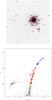 |
Fig. 1 Upper panel: a 15′ × 15′ DSS map of NGC 5634 with north up and east left. Our targets are colour-coded as observed with GIRAFFE (in red) and UVES (in blue). Non member stars are indicated in green. Lower panel: V,V−I CMD (from B02) with FLAMES targets indicated by larger, coloured symbols (subsample UVES: filled blue dots and subsample GIRAFFE filled and open red squares for RGB and AGB stars, respectively). Green crosses represent non member stars. |
3.1. FLAMES spectra
Log of FLAMES observations.
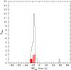 |
Fig. 2 Histogram of heliocentric RVs (the filled red histogram indicates the seven UVES stars). The cluster stars are easily identified, with RV near − 16 km s-1. |
NGC 5634 was observed with the multi-object spectrograph VLT/FLAMES (Pasquini et al. 2002) in the ESO program 093.B-0583 (PI A. Bragaglia). The observations, in priority B, were performed in service mode; a log is presented in Table 1. Unfortunately, only less than half of the planned observations were actually completed. We only have four exposures (out of the six requested) taken with the GIRAFFE high-resolution setup HR11 (R = 24 200), containing the 5682–88 Å Na i doublet; no exposures with the HR13 setup, containing the forbidden [O i] lines, are available. The GIRAFFE observations of 38 stars were coupled with the spectra of seven stars obtained with the high-resolution (R = 47 000) UVES (Dekker et al. 2000) 580 nm setup (λλ ≃ 4800−6800 Å). Information on the 45 stars (ID, coordinates, magnitudes and RVs) is given in Table 2.
The reduced GIRAFFE spectra were obtained from the ESO archive (request 168 411) as part of the Advanced Data Products (ADP). The UVES spectra were reduced by us using the ESO pipeline for UVES-FIBRE data, which takes care of bias and flat field correction, order tracing, extraction, fibre transmission, scattered light, and wavelength calibration. We then used IRAF2 routines on the 1d, wavelength-calibrated individual spectra to subtract the (average) sky, measure the heliocentric RV, shift to zero RV and combine all the exposures for each star.
In Fig. 2, we show the histogram of the RVs; the cluster signature is evident and we identitied 43 of the 45 observed targets as cluster members on the basis of their RV. One star has no measured RV and one has a discrepant RV and was labelled as a non-cluster member. Star 151, initially considered a member of the cluster due to its RV, was afterwards classified a non-member following the abundance analysis and then disregarded. The average, heliocentric RV for each star is given in Table 2, together with its rms. For member stars, we found an average RV of − 16.07 km s-1 (with σ = 3.98). This value is in excellent agreement with the average RV (− 16.7 km s-1, σ = 5.5) found by S15 from two stars, but not with the older literature value (− 45.1 km s-1) listed in Harris (1996, 2010 web update), as already discussed in S15, or with the value of − 29.6 (σ = 39.1) km s-1 in Dias et al. (2016), that was however obtained on much-lower-resolution spectra.
3.2. Atmospheric parameters
We retrieved the 2MASS magnitudes (Skrutskie et al. 2006) of the 43 RV-member stars; K magnitudes, 2MASS identification and quality flag are given in Table 2. Following our well tested procedure (for a detailed description, see Carretta et al. 2009a,b), effective temperatures Teff were derived using an average relation between apparent magnitudes and first-pass temperatures from V−K colours and the calibrations of Alonso et al. (1999, 2001). This method allowed us to decrease the star-to-star errors in abundances due to uncertainties in temperature. The adopted reddening E(B−V) = 0.05, distance modulus (m−M)V = 17.16, and input metallicity [Fe/H] =−1.88 are taken from Harris (1996, 2010 web update). Gravities were obtained from apparent magnitudes and distance modulus, assuming the bolometric corrections from Alonso et al. (1999). We adopted a mass of 0.85 M⊙ for all stars and Mbol, ⊙ = 4.75 as the bolometric magnitude for the Sun, as in our previous studies.
Since only one of the two requested GIRAFFE setups was done, only a limited number of Fe transitions from our homogeneous line list (from Gratton et al. 2003) were available for stars with GIRAFFE spectra, and this affected the abundance analysis. Fortunately, the seven stars with spectra taken with UVES were chosen among those in the brightest magnitude range, close to the RGB tip (see Fig. 1) and did not suffer excessively for the lack of all planned observations. The S/N values per pixel range from 90 to 40 from the brightest down to the faintest of our UVES sample stars. The median S/N for the 35 member stars with GIRAFFE spectra is 58 at λ ~ 5600 Å. Literature high-resolution spectra are available only for two stars in this cluster (S15), therefore even such a small sample represents a significant improvement.
We measured the equivalent widths (EW) of iron and other elements using the code ROSA (Gratton 1988) as described in detail in Bragaglia et al. (2001). We employed spectrum synthesis for a number of elements (see Sect. 4.3). For the UVES spectra, we eliminated trends in the relation between abundances from Fe i lines and expected line strength (Magain 1984) to obtain values of the microturbulent velocity vt. However, for the 35 member stars with GIRAFFE HR11 spectra too few Fe lines were available and we generally adopted a relation with the star’s gravity: vt = −0.31log g + 2.19, derived from our previous analyses, apart from a few cases. Finally, we interpolated within the Kurucz (1993) grid of model atmospheres (with overshooting on) to derive the final abundances, adopting, for each star, the model with the appropriate atmospheric parameters and whose abundances matched those derived from Fe i lines. The adopted atmospheric parameters (Teff, log g, [A/H], and vt) are listed in Table 3 together with iron abundances. Figure 3 shows the run of [Fe/H] from neutral and ionised transitions as a function of the effective temperature; no trend is visible in either case. We find, for NGC 5634, an average metallicity [Fe/H] =−1.867 ± 0.019 dex (rms = 0.050 dex) and − 1.903 ± 0.009 dex (rms = 0.025 dex) from the seven stars with UVES spectra for neutral and ionised lines, respectively. The average difference − 0.036 ± 0.015 dex (rms = 0.040) dex is not significant.
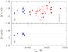 |
Fig. 3 Run of the iron abundances as a function of the effective temperature for the seven UVES stars (blue circles) and stars with GIRAFFE spectra (red circles). Abundances from singly ionised Fe lines are shown in the lower panel for UVES stars only. Internal error bars are also displayed (for the UVES sample on the left corner, for the GIRAFFE sample in the right corner). The dotted line is the average abundance derived from the UVES spectra. |
The average value is in very good agreement with the mean metallicity that we derived from the analysis of the 35 stars with GIRAFFE spectra: [Fe/H] =−1.869 ± 0.016 dex (σ = 0.093 dex). The larger dispersion is ultimately mostly due to the limited number of Fe lines available in the spectral range of the HR11 setup, hampering a better derivation of the parameters (see also Sect. 4).
Adopted atmospheric parameters and derived metallicity.
4. Abundances
Besides Fe, we present here abundances of O, Na, Mg, Al, Si, Ca, Sc, Ti (both from neutral and singly ionised transitions), V, Cr (from both Cr i and Cr ii lines), Mn, Co, Ni, Zn, Cu, Y, Zr, Ba, La, Ce, Nd and Eu obtained from UVES spectra. For stars in the GIRAFFE sample, we only derived abundances of one proton-capture element (Na), three α-capture elements (Mg, Si, and Ca), and three elements of the iron-group (Sc, V, and Ni). The abundances were derived using EWs for all species except Cu and neutron-capture elements. The atomic data for the lines and the solar reference values come from Gratton et al. (2003). The Na abundances were corrected for departure from local thermodynamical equilibrium according to Gratton et al. (1999), as in all the other papers of our FLAMES survey. Corrections to account for the hyperfine structure were applied to Sc, V, Mn (references are in Gratton et al. 2003) and Y.
To estimate the error budget, we closely followed the procedure described in Carretta et al. (2009a,b). Table 4 provides the sensitivities of abundance ratios to uncertainties in atmospheric parameters and EWs, and the internal and systematic errors relative to the abundances from UVES spectra. The same quantities are listed in Table 5 for abundances from GIRAFFE spectra. In this second case, to have a conservative estimate of the internal error in vt, we adopted the quadratic sum of the GIRAFFE internal errors for the metal-poor GCs in our FLAMES survey: NGC 4590, NGC 6397, NGC 6805, NGC 7078, NGC 7099 (Carretta et al. 2009a), NGC 6093 (Carretta et al. 2015) and NGC 4833 (Carretta et al. 2014b).
The sensitivities were obtained by repeating the abundance analysis for all stars, while changing one atmospheric parameter at a time, then taking the average. The amount of variation in the input parameters used in the sensitivity computations is given in the table headers.
On our UVES metallicity scale (see Carretta et al. 2009c), the average metal abundance for NGC 5634 is therefore [Fe/H] =−1.867 ± 0.019 ± 0.065 dex (σ = 0.050 dex, 7 stars), where the first and second error bars refer to statistical and systematic errors, respectively.
The abundance ratios for proton-capture elements are given in Table 6 for UVES spectra, together with the number of lines used and rms scatter. All O abundances are detections; no measure of O abundance in star 5634-13 was possible because the forbidden line [O I] 6300.31 Å was affected by sky contamination. For stars 5634-2 and 5634-9, only upper limits could be measured for Al.
Sensitivities of abundance ratios to variations in the atmospheric parameters and to errors in the equivalent widths, and errors in abundances for stars of NGC 5634 observed with UVES.
Sensitivities of abundance ratios to variations in the atmospheric parameters and to errors in the equivalent widths, and errors in abundances for stars of NGC 5634 observed with GIRAFFE.
Light element abundances.
α element abundances.
Iron-peak abundances.
Neutron-capture abundances.
Abundances from GIRAFFE spectra.
Mean abundances in NGC 5634.
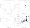 |
Fig. 4 Relations among proton-capture elements in stars of NGC 5634 observed with UVES (filled blue circles). Empty squares in the lower-right panel are stars in 24 GCs from Carretta et al. (2009a,b, 2010b,c, 2011, 2013, 2014b, 2015), and asterisks are stars in NGC 2808 from Carretta (2015). In each panel the error bars represent internal errors. |
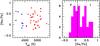 |
Fig. 5 Left-hand panel: [Na/Fe] ratios as a function of the temperature in stars observed with UVES (blue squares) and GIRAFFE (red circles). Right-hand panel: histogram of the [Na/Fe] ratios, where the line indicates the division between P and I stars, based on our usual separation at [Na/Fe]min + 0.3. |
Abundances of α-capture, iron-peak and neutron-capture elements for the individual stars are listed in Tables 7, and 8, and 9, respectively, for the seven stars with UVES spectra. Except for iron, all the abundances derived for stars observed with GIRAFFE are listed in Table 10. For these 35 stars, all the element ratios are in reference to the average iron abundance [Fe/H] =−1.87 dex. Finally, in Table 11, the mean abundances in NGC 5634 are summarised.
We cross-matched our stars with the nine objects in Dias et al. (2016) and found only three in common. Stars # 9, 54, and 87 in our sample are within 1′′ of stars # 11, 8 and 7 in their list and have reasonably similar V magnitudes (theirs are instrumental values) and atmospheric parameters. We do not dwell on the comparison since their results are based on lower-resolution spectra. However, their cluster average metallicity agrees with ours within the error bars and their Mg abundance and [α/Fe] are in very good agreement.
We also have three stars in common with the APOGEE survey (Holtzman et al. 2015); however parameters were presented only for two of the stars in DR12. Furthermore, a straightforward comparison is difficult because of different model atmospheres, spectral ranges and line list, and adopted methods.
Limiting the comparison to the optical range, ours is the second high-resolution optical spectroscopic study of this cluster. S15 used a full spectroscopic parameter determination for the two stars they analysed in NGC 5634. Had we used their atmospheric parameters for star 5634-2, in common with that study and observed with similar resolution and wavelength coverage, we would have obtained, on average, higher abundances by 0.003 ± 0.016 dex (σ = 0.060 dex) from 14 neutral species and lower by − 0.049 ± 0.022 dex (σ = 0.058 dex) from 7 singly ionised species, once our solar reference abundances from Gratton et al. (2003) are homogeneously adopted.
NGC 5634 seems to be a homogeneous cluster, as far as most elements are concerned. By comparing the expected observational uncertainty due to errors affecting the analysis (the internal errors in Table 4) with the observed dispersion (the standard deviation about the mean values in Table 11), we can evaluate whether or not there is an intrinsic or cosmic scatter for a given element among stars in NGC 5634. This exercise was made using the more accurate abundances from UVES spectra; it is essentially equivalent to compute the “spread ratio” introduced by Cohen (2004) and shows that there is only evidence for an intrinsic spread for O, Na, and Al, while Fe, Y, and Eu show only a “possible” spread.
However, we do not consider the spread in Fe to be real, since in this case the observational uncertainty is very small due to the large number of measured lines in UVES spectra. On the other extreme, when the abundance of a given species is based on a very limited number of lines, the spread ratio may be high due to bias (see Cohen 2004, for a discussion), as in the case of Y and Eu. Moreover, all five determinations of Eu abundances from the line at 6437 Å are upper limits. Had we considered only the detections (from the Eu 6645 Å line), the spread ratio would be <1, implying no intrinsic spread for Eu in NGC 5634.
In conclusion, the overall pattern of the chemical composition shows that NGC 5634 is a normal GC, where most elements do not present any intrinsic star-to-star variation, except for those involved in proton-capture reactions in H burning at a high temperature, such as O, Na, and Al, and as commonly observed in GCs (see Gratton et al. 2012).
4.1. The light elements
The relations among proton-capture elements in stars of NGC 5634 are summarised in Fig. 4 for the UVES sample. Abundances of Na are also anticorrelated with O abundances in NGC 5634 (upper left panel), confirming the findings by S15 with a sample three times larger. This cluster shares the typical Na-O anticorrelation, the widespread chemical signature of multiple stellar populations in MW GCs. Within the important limitations of small number statistics, two stars have distinctly larger Na content and lower O abundance than the other four stars.
According to the homogeneous criteria used by our group to define stellar generations in GCs (see Carretta et al. 2009a), the two stars with the highest Na abundance would be second generation stars of the intermediate I component, while the other four giants belong to the first generation in NGC 5634 and reflect the primordial P fraction, with the typical pure nucleosynthesis by type II SNe (the average abundances for these stars are [Na/Fe] = 0.017 dex, σ = 0.151 dex and [O/Fe] = 0.361 dex, σ = 0.102 dex). The star with only a Na abundance would also be classified as a first generation star, due to its low ratio [Na/Fe] = + 0.052 dex.
We note that the two stars analysed by S15 show (anticorrelated) spreads in O and Na exceeding the estimated observational uncertainties; evidence that prompted the authors to claim a Na-O anticorrelation in NGC 5634. Nevetheless, both stars would fall among our first generation stars, either if the original abundances or those corrected for different solar abundances are adopted. In our data, the observed spread in O for the stars of the P component is comparable with the expected uncertainty due to the analysis, whereas the spread in Na formally corresponds to 1.7σ. We cannot totally exclude a certain amount of intrinsic spread among proton-capture elements in the first generation stars in NGC 5634, supporting previous findings by S15 based on the Na abundances of their two stars, photometrically very similar.
The impression is supported by the upper-right and lower-left panels in Fig. 4: no significant star-to-star variation is observed for Mg, while the Al abundances cover a relatively large range, which is only a lower limit since for two P stars, only upper limits to the Al abundances could be measured.
The lack of any extreme abundance variation in Mg is strongly confirmed by the lower-right panel, where we compare abundances of Ca and Mg in NGC 5634 with the values found in our homogeneous survey of 25 GCs. The stars analysed in NGC 5634 follow the trend of cluster stars with no extreme Mg depletion (see also S15).
To gain a more robust estimate of the fraction of first and second generation stars in NGC 5634, we may resort to the large statistics provided by Na abundances of the combined UVES+GIRAFFE sample. We cannot distinguish between second generation stars with intermediate and extreme composition (this would require knowledge of O abundances also), but the definition of the primordial P fraction in a GC simply rests on Na abundances (Carretta et al. 2009a).
Using the total sample and separating at [Na/Fe]min+0.3 dex, the fraction of P stars in NGC 5634 is 38 ± 10%, while the fraction of the second generation stars is 62 ± 12%, where the associated errors are due to Poisson statistics. These fractions are not very different from the average of what is found in most GCs (see e.g. Carretta et al. 2009a, 2010a).
4.2. Elements up to iron peak
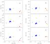 |
Fig. 6 Abundance ratios of α- and iron-peak elements derived from UVES spectra in NGC 5634 as a function of the metallicity (filled blue circles). Also plotted are the average values from Table 11 of Carretta et al. (2014a) relative to the Sgr nucleus (black asterisk, Carretta et al. 2010b), to M 54 (black empty circle, Carretta et al. 2010b), to Pal 12 (red filled square, Cohen 2004), to Terzan 7 (orange filled star, Sbordone et al. 2007), to Terzan 8 (filled light-blue triangle, Carretta et al. 2014a) and to Arp 2 (green empty square, Mottini et al. 2008). Internal error bars refer to our UVES sample. |
In Fig. 6, we summarise the chemical composition of NGC 5634 as far as α-elements and iron-peak elements are concerned, using the individual values derived for stars with UVES spectra, as a function of the metallicity. As a comparison, we also plot the average value relative to the Sgr nucleus ([Fe/H] =−0.74 dex, Carretta et al. 2010b) and to the five GCs confirmed members of the Sgr dwarf galaxy: M 54 ([Fe/H] =−1.51 dex, Carretta et al. 2010b), Terzan 8 ([Fe/H] =−2.27 dex, Carretta et al. 2014a), Arp 2 ([Fe/H] =−1.80 dex, Mottini et al. 2008), Pal 12 ([Fe/H] =−0.82 dex, Cohen 2004) and Terzan 7 ([Fe/H] =−0.61 dex, Sbordone et al. 2007). In the last three cases, the values were corrected to the scale of solar abundances presently used (Gratton et al. 2003).
Abundances of stars in NGC 5634 seem to be in good agreement with the metal-poor GCs associated to Sgr. Of course, by itself, this is not clear-cut proof of the membership of NGC 5634 to Sgr rather than to the Milky Way, since at this low metal abundance, the overall chemical pattern of the α- and iron-peak elements simply reflects the typical floor of elemental abundances established by the interplay of core-collapse and type Ia supernovae (see e.g. Wheeler et al. 1989). This pattern is also supported by the abundances derived from GIRAFFE spectra (Table 11). In Sect. 5, we discuss further elements to support the connection with Sgr dSph.
4.3. Neutron-capture elements
Abundances for six neutron-capture elements in the UVES sample are listed in Table 9 and their cluster means are in Table 11. Ba ii and Nd ii lines could be treated as single unblended absorbers, so they were treated with EW analyses. Transitions of the other four neutron-capture elements had complications due to blending, hyperfine, or isotopic substructure and so were subjected to synthetic spectrum analyses. The elemental means appear to be straightforward: the light n-capture elements Y and Zr are slightly under- and over-abundant, respectively, with respect to Fe, the traditional s-process rare-earth elements Ba and La have solar abundances, the r-process dominant Eu is overabundant by approximately a factor of four and the r-/s-transition element Nd is overabundant by almost a factor of three. Here, we comment on a number of aspects of our derived n-capture abundances.
Our derived Ba and Eu abundances are in reasonable agreement with those reported by S15. Barium is not the optimal element to assess the abundances of the low-Z end of the rare earths because all Ba ii lines are strong and thus less sensitive to abundance than are weaker lines. Fortunately, abundances derived from weak La ii transitions are not in severe disagreement with the Ba values.
We determined Y abundances for our UVES sample from the Y ii line at 5200.4 Å, for homogeneity with what we did for Ter 8 and other GCs in our sample (e.g. Carretta et al. 2014a). The cluster mean abundance from this transition is [Y/Fe] = − 0.083 (σ = 0.119, 7 stars; see Table 9). The star-to-star scatter is relatively large, but almost all stars have [Y/Fe] ≲ 0. Sbordone et al. (2015) reported much lower Y abundance in NGC 5634: [Y/Fe] =−0.40 from Star 2 and −0.33 from Star 3.
Star 2 in our study yielded [Y/Fe] = − 0.077 from the synthesis of the 5200 Å line. To investigate this +0.32 dex offset in [Y/Fe] with respect to S15, we synthesised other Y ii lines in Star 2 with the line analysis code MOOG (Sneden 1973). Using the transition probabilities of Hannaford et al. (1982) and Biémont et al. (2011), we used ten Y ii lines to derive ⟨ [ log ϵ(Y)]⟩=+0.25 ± 0.03 (σ = 0.08 dex). Adopting log ϵ(Y)⊙ = 2.21 (Asplund et al. 2009) leads to a mean value of [Y/H]=−1.96 or [Y/Fe]=−0.09 (with the cluster mean [Fe/H] =−1.87), in good agreement with the value derived from the 5200 Å line alone.
For Star 2, we display our synthetic/observed spectrum match in Fig. 7. From this line, our best estimate is log ϵ(Y)= + 0.30. We conclude that the spectrum synthesis of the line 5200 Å alone allows us to derive a relatively good estimate of the Y content. In general, we do not find substantial Y deficiencies for any of our UVES samples in NGC 5634.
As suggested by the referee, we used the line profile for each synthesised line of Y ii published by S15 for star 2 and fitted them with our code and linelist. We obtained very consistent abundances from these four lines (log ϵ = + 0.21 ± 0.04 dex, σ = 0.09 dex and log ϵ = + 0.28 ± 0.03 dex, σ = 0.06 dex, with and without continuum scattering). This exercise would give an offset 0.43–0.50 dex with respect to the value of S15. At present, we cannot provide an explanation for the difference.
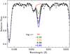 |
Fig. 7 Synthetic spectra for the Y ii line 5200.4 Å. Filled circles indicate the observed spectrum of star 5634-2. |
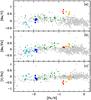 |
Fig. 8 Abundance ratios of neutron-capture elements Y and Ba as a function of metallicity. Grey filled circles are Galactic field stars from the compilation by Venn et al. (2004). The other symbols are as in Fig. 6: Pal 12 (red filled squares, Cohen 2004), Terzan 7 (orange filled stars, Sbordone et al. 2007), Terzan 8 (filled light-blue triangles, Carretta et al. 2014a) and Arp 2 (green empty squares, Mottini et al. 2008). |
Derived Ba and Y abundances in NGC 5634 are in good agreement with the trend defined by Galactic field stars of similar (low) metal abundances, as shown in Fig. 8. Again, the metal-rich GCs associated to the Sgr dwarf stand out with respect to the Galactic field stars, while NGC 5634 cannot be distinguished from its chemical composition alone, as also occurs for Terzan 8, the classical metal-poor globular cluster of the family of GCs in Sgr.
Here we are comparing our NGC 5634 abundance ratios with those of other Sgr clusters. In the following section we consider the kinematics of this cluster in order to more firmly establish its membership in the Sgr family.
5. Connection with the Sagittarius dSph and internal kinematics
As introduced in Sect. 1, NGC 5634 is suggested to have formed in the Sgr dSph and then accreted by the Milky Way during the subsequent tidal disruption of its host galaxy (Bellazzini et al. 2002; Law & Majewski 2010a). In this scenario, this GC is expected to follow an orbit similar to that of its parent galaxy and to be embedded in its stream. We checked this hypothesis by comparing the position and systemic motion of NGC 5634 with the prediction of the Sagittarius model by Law & Majewski (2010b). Among the three models presented in that paper, we used the one assuming a prolate (q = 1.25) Galactic halo, which provides a better fit to the observational constraints on the location and kinematics of the Sagittarius stream stars. The distribution in the heliocentric distance-radial velocity plane of particles within 5deg from the present-day position of NGC 5634 is shown in Fig. 9. It is apparent that in this diagram, NGC 5634 lies well within a clump of Sagittarius particles. These particles belong to the trailing arm of its stream and have been lost by the satellite between 3 and 7 Gyr ago. This is consistent with what was found by B02 and Law & Majewski (2010a), even if they used a slightly different systemic radial velocity for this cluster (–44.4 km s-1).
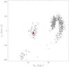 |
Fig. 9 Position and velocity of NGC 5634 (large filled red dot) compared to a Sgr model (see text for details). |
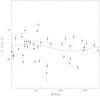 |
Fig. 10 Systemic rotation of NGC 5634: the best-fit solution is compatible with negligible rotation. |
5.1. Internal kinematics
The present data represent the most extensive set of radial velocities for NGC 5634 and could be useful for studying the internal kinematics of this cluster. As a first step, we test the presence of systemic rotation. For this purpose, in Fig. 10, the RVs of the 42 bona fide members are plotted against their position angles. The best-fit sinusoidal curve indicates a rotation amplitude of Arot sini = 1.08 ± 1.34 km s-1, compatible with no significant rotation.
We then used our RV dataset to estimate the dynamical mass of the system. For this purpose, we fitted the distribution of RVs with a set of single and multimass King-Michie models (King 1966; Gunn & Griffin 1979). In particular, for each model, we tuned the model mass to maximize the log-likelihood  (1)where N(=42) is the number of available RVs, vi and ϵi are the radial velocity of the ith star and its associated uncertainty and σi is the line-of-sight velocity dispersion predicted by the model at the distance from the cluster centre of the ith star. The best-fit single mass model provides a total mass of 1.64 × 10⁵M⊙. This quantity, however, needs to be considered a lower limit to the actual total mass because of the effect of two-body relaxation affecting this estimate. Indeed, RGB stars (i.e. those for which RVs are available) are, on average, more massive than typical cluster stars and are therefore expected to become kinematically colder and more concentrated than the latter after a timescale comparable to the half-mass relaxation time. To account for this effect, we performed the same analysis adopting a set of multimass models with various choices of the present-day mass function. In particular, we adopted a power-law mass function with indices ranging from –2.35 (i.e. Salpeter 1955) to 0. We adopted the prescriptions for dark remnants and binaries of Sollima et al. (2012) assuming a binary fraction of 10% and a flat distribution of mass-ratios. The derived masses turn out to be 1.72, 1.82, 2.04 and 1.93 × 10⁵M⊙ for mass function slopes of α = 0,−1,−2 and − 2.35, respectively, with a typical uncertainty of ~ 4.5 × 10⁴M⊙. By assuming the absolute magnitude MV = −7.69 listed for this cluster in the Harris catalog (1996, 2010 edition), the corresponding M/L ratios are 1.68, 1.79, 2.01 and 1.90, respectively. Significantly larger M/L ratios (by a factor 1.24) are instead obtained if the integrated magnitude by McLaughlin & van der Marel (2005) is adopted.
6. Summary and conclusions
As part of our homogeneous study of GCs, we obtained FLAMES spectra of 42 member stars in the cluster NGC 5634, associated to the Sgr dSph, in particular to one of the arms of the Sgr stream. We measured elemental abundances for many elements in the UVES spectra of seven RGB stars and of several elements in the GIRAFFE spectra of 35 (mainly) RGB and AGB stars (see Fig. 1).
We found clear evidence of multiple stellar populations in this cluster, indicated by the classical (anti)correlations between light elements (O, Na; Mg and Al). Although we could not completely characterise these anticorrelations due to a lack of oxygen abundance for all GIRAFFE targets, we can divide the observed stars into primordial P and Intermediate I fractions (Carretta et al. 2009a,b) simply using their Na abundance. Apparently, for this Sgr cluster, the fraction of first and second generation stars is not dramatically different from typical values found in MW GCs from spectroscopy (e.g. Carretta et al. 2009a, 2010a; Johnson & Pilachowski 2012).
We support the connection between NGC 5634 and the Sgr dSph (B02, Law & Majewski 2010a) both on the basis of the cluster RV and position and on the chemical abundances. The second piece of evidence is not, however, clearcut, since NGC 5634 resembles both MW and low-metallicity Sgr GCs in α and neutron-capture elements. We do not confirm the very low Y ii abundance found by S15.
This study adds yet another confirmation of the ubiquitous presence of light-element anticorrelations, that is, multiple populations, among old and massive GCs, independent of their formation place. Metal-poor GCs apparently formed following the same chain of events regardless of their birth environment was the central Galaxy (Milky Way) or its most prominent disrupting dwarf satellite (Sgr).
IRAF is distributed by the National Optical Astronomical Observatory, which are operated by the Association of Universities for Research in Astronomy, under contract with the National Science Foundation.
Acknowledgments
We thank P. Montegriffo for his software CataPack, Michele Bellazzini for useful comments, and the referee Luca Sbordone for his thoughful review. Support for this work has come in part from the US NSF grant AST-1211585. This research has made use of Vizier and SIMBAD, operated at CDS, Strasbourg, France, and NASA’s Astrophysical Data System. The Guide Star Catalogue-II is a joint project of the Space Telescope Science Institute and the Osservatorio Astronomico di Torino. Space Telescope Science Institute is operated by the Association of Universities for Research in Astronomy, for the National Aeronautics and Space Administration under contract NAS5-26555. The participation of the Osservatorio Astronomico di Torino is supported by the Italian Council for Research in Astronomy. Additional support is provided by European Southern Observatory, Space Telescope European Coordinating Facility, the International GEMINI project and the European Space Agency Astrophysics Division.This publication makes use of data products from the Two Micron All Sky Survey, which is a joint project of the University of Massachusetts and the Infrared Processing and Analysis Center/California Institute of Technology, funded by the National Aeronautics and Space Administration and the National Science Foundation.
References
- Alonso, A., Arribas, S., & Martínez-Roger, C. 1999, A&AS, 140, 261 [NASA ADS] [CrossRef] [EDP Sciences] [Google Scholar]
- Alonso, A., Arribas, S., & Martínez-Roger, C. 2001, A&A, 376, 1039 [NASA ADS] [CrossRef] [EDP Sciences] [Google Scholar]
- Asplund, M., Grevesse, N., Sauval, A. J., & Scott, P. 2009, ARA&A, 47, 481 [NASA ADS] [CrossRef] [Google Scholar]
- Bastian, N., Cabrera-Ziri, I., & Salaris, M. 2015, MNRAS, 449, 3333 [NASA ADS] [CrossRef] [Google Scholar]
- Bellazzini, M., Ferraro, F. R., & Ibata, R. 2002, AJ, 124, 915 (B02) [NASA ADS] [CrossRef] [Google Scholar]
- Bellazzini, M., Ferraro, F. R., & Ibata, R. 2003, AJ, 125, 188 [NASA ADS] [CrossRef] [Google Scholar]
- Biémont, É., Blagoev, K., Engström, L., et al. 2011, MNRAS, 414, 3350 [NASA ADS] [CrossRef] [Google Scholar]
- Bragaglia, A., Carretta, E., Gratton, R. G., et al. 2001, AJ, 121, 327 [NASA ADS] [CrossRef] [Google Scholar]
- Bragaglia, A., Gratton, R. G., Carretta, E., et al. 2012, A&A, 548, A122 [NASA ADS] [CrossRef] [EDP Sciences] [Google Scholar]
- Bragaglia, A., Sneden, C., Carretta, E., et al. 2014, ApJ, 796, 68 [NASA ADS] [CrossRef] [Google Scholar]
- Bragaglia, A., Carretta, E., Sollima, A., et al. 2015, A&A, 583, A69 [NASA ADS] [CrossRef] [EDP Sciences] [Google Scholar]
- Carretta, E. 2015, ApJ, 810, 148 [NASA ADS] [CrossRef] [Google Scholar]
- Carretta, E., Bragaglia, A., Gratton, R. G., et al. 2009a, A&A, 505, 117 [NASA ADS] [CrossRef] [EDP Sciences] [Google Scholar]
- Carretta, E., Bragaglia, A., Gratton, R. G., & Lucatello, S. 2009b, A&A, 505, 139 [NASA ADS] [CrossRef] [EDP Sciences] [Google Scholar]
- Carretta, E., Bragaglia, A., Gratton, R. G., D’Orazi, V., & Lucatello, S. 2009c, A&A, 508, 695 [NASA ADS] [CrossRef] [EDP Sciences] [Google Scholar]
- Carretta, E., Bragaglia, A., Gratton, R. G., et al. 2010a, A&A, 516, 55 [NASA ADS] [CrossRef] [EDP Sciences] [Google Scholar]
- Carretta, E., Bragaglia, A., Gratton, R. G., et al. 2010b, A&A, 520, 95 [Google Scholar]
- Carretta, E., Gratton, R. G., Lucatello, S., et al. 2010c, ApJ, 722, L1 [NASA ADS] [CrossRef] [Google Scholar]
- Carretta, E., Lucatello, S., Gratton, R. G., Bragaglia, A., & D’Orazi, V. 2011, A&A, 533, 69 [NASA ADS] [CrossRef] [EDP Sciences] [Google Scholar]
- Carretta, E., Bragaglia, A., Gratton, R. G., et al. 2013, A&A, 557, A138 [NASA ADS] [CrossRef] [EDP Sciences] [Google Scholar]
- Carretta, E., Bragaglia, A., Gratton, R. G., et al. 2014a, A&A, 561, A87 [NASA ADS] [CrossRef] [EDP Sciences] [Google Scholar]
- Carretta, E., Bragaglia, A., Gratton, R. G., et al. 2014b, A&A, 564, A60 [NASA ADS] [CrossRef] [EDP Sciences] [Google Scholar]
- Carretta, E., Bragaglia, A., Gratton, R. G., et al. 2015, A&A, 578, A116 [NASA ADS] [CrossRef] [EDP Sciences] [Google Scholar]
- Cohen, J. G. 2004, AJ, 127, 1545 [NASA ADS] [CrossRef] [Google Scholar]
- Decressin, T., Meynet, G., Charbonnel, C., Prantzos, N., & Ekstrom, S. 2007, A&A, 464, 1029 [NASA ADS] [CrossRef] [EDP Sciences] [Google Scholar]
- Dekker, H., D’Odorico, S., Kaufer, A., Delabre, B., & Kotzlowski, H. 2000, Proc. SPIE, 4008, 534 [Google Scholar]
- de Mink, S. E., Pols, O. R., Langer, N., & Izzard, R. G. 2009, A&A, 507, L1 [NASA ADS] [CrossRef] [EDP Sciences] [Google Scholar]
- Denisenkov, P. A., & Denisenkova, S. N. 1989, Astron. Tsirkulyar, 1538, 11 [Google Scholar]
- Denissenkov, P. A., & Hartwick, F. D. A. 2014, MNRAS, 437, L21 [NASA ADS] [CrossRef] [Google Scholar]
- Dias, B., Barbuy, B., Saviane, I., et al. 2016, A&A, 590, A9 [NASA ADS] [CrossRef] [EDP Sciences] [Google Scholar]
- Gratton, R. G. 1988, Rome Obs. Preprint Ser., 29 [Google Scholar]
- Gratton, R. G., Carretta, E., Eriksson, K., & Gustafsson, B. 1999, A&A, 350, 955 [NASA ADS] [Google Scholar]
- Gratton, R. G., Bonifacio, P., Bragaglia, A., et al. 2001,A&A, 369, 87 [Google Scholar]
- Gratton, R. G., Carretta, E., Claudi, R., Lucatello, S., & Barbieri, M. 2003, A&A, 404, 187 [NASA ADS] [CrossRef] [EDP Sciences] [Google Scholar]
- Gratton, R. G., Carretta, E., & Bragaglia, A. 2012, A&ARv, 20, 50 [CrossRef] [Google Scholar]
- Gunn, J. E., & Griffin, R. F. 1979, AJ, 84, 752 [NASA ADS] [CrossRef] [Google Scholar]
- Hannaford, P., Lowe, R. M., Grevesse, N., Biemont, E., & Whaling, W. 1982, ApJ, 261, 736 [NASA ADS] [CrossRef] [Google Scholar]
- Harris, W. E. 1996, AJ, 112, 1487 [NASA ADS] [CrossRef] [Google Scholar]
- Holtzman, J. A., Shetrone, M., Johnson, J. A., et al. 2015, AJ, 150, 148 [NASA ADS] [CrossRef] [Google Scholar]
- Johnson, C. I., & Pilachowski, C. A. 2012, ApJ, 754, L38 [NASA ADS] [CrossRef] [Google Scholar]
- Johnson, J. A., Ivans, I. I., & Stetson, P. B. 2006, ApJ, 640, 801 [NASA ADS] [CrossRef] [Google Scholar]
- Kraft, R. P. 1994, PASP, 106, 553 [NASA ADS] [CrossRef] [Google Scholar]
- King, I. R. 1966, AJ, 71, 64 [Google Scholar]
- Kurucz, R. L. 1993, CD-ROM 13, Smithsonian Astrophysical Observatory, Cambridge [Google Scholar]
- Langer, G. E., Hoffman, R., & Sneden, C. 1993, PASP, 105, 301 [NASA ADS] [CrossRef] [Google Scholar]
- Larsen, S. S., Brodie, J. P., Grundahl, F., & Strader, J. 2014,ApJ, 797, 15 [Google Scholar]
- Law, D. R., & Majewski, S. R. 2010a, ApJ, 718, 1128 [NASA ADS] [CrossRef] [Google Scholar]
- Law, D. R., & Majewski, S. R. 2010b, ApJ, 714, 229 [NASA ADS] [CrossRef] [Google Scholar]
- Letarte, B., Hill, V., Jablonka, P., et al. 2006, A&A, 453, 547 [NASA ADS] [CrossRef] [EDP Sciences] [Google Scholar]
- Maccarone, T. J., & Zurek, D. R. 2012, MNRAS, 423, 2 [NASA ADS] [CrossRef] [Google Scholar]
- Magain, P. 1984, A&A, 134, 189 [NASA ADS] [Google Scholar]
- McLaughlin, D. E., & van der Marel, R. P. 2005, ApJS, 161, 304 [NASA ADS] [CrossRef] [Google Scholar]
- Milone, A., Piotto, G., Bedin, L., et al. 2012, ApJ, 744, 58 [NASA ADS] [CrossRef] [Google Scholar]
- Mottini, M., Wallerstein, G., & McWilliam, A. 2008, AJ, 136, 614 [NASA ADS] [CrossRef] [Google Scholar]
- Mucciarelli, A., Origlia, L., Ferraro, F. R., & Pancino, E. 2009, ApJ, 695, L134 [NASA ADS] [CrossRef] [Google Scholar]
- Noguchi, K., Aoki, W., Kawanomoto, S., et al. 2002, PASJ, 54, 855 [NASA ADS] [CrossRef] [Google Scholar]
- Pasquini, L., Avila, G., Blecha, A., et al. 2002, The Messenger, 110, 1 [NASA ADS] [Google Scholar]
- Prantzos, N., Charbonnel, C., & Iliadis, C. 2007, A&A, 470, 179 [NASA ADS] [CrossRef] [EDP Sciences] [Google Scholar]
- Salpeter, E. E. 1955, ApJ, 121, 161 [Google Scholar]
- Sbordone, L., Bonifacio, P., Buonanno, R., et al. 2007, A&A, 465, 815 [NASA ADS] [CrossRef] [EDP Sciences] [Google Scholar]
- Sbordone, L., Salaris, M., Weiss, A., & Cassisi, S. 2011, A&A, 534, A9 [NASA ADS] [CrossRef] [EDP Sciences] [Google Scholar]
- Sbordone, L., Monaco, L., Moni Bidin, C., et al. 2015, A&A, 579, A104 (S15) [NASA ADS] [CrossRef] [EDP Sciences] [Google Scholar]
- Skrutskie, M. F., et al. 2006, AJ, 131, 1163 [NASA ADS] [CrossRef] [Google Scholar]
- Sneden, C. 1973, ApJ, 184, 839 [NASA ADS] [CrossRef] [Google Scholar]
- Sneden, C. 2000, in The Galactic Halo: From Globular Cluster to Field Stars, Proc. 35th Liege Int. Astrophys. Colloquium, 1999, eds. A. Noels, P. Magain, D. Caro, et al., Liege, Belgium, 159 [Google Scholar]
- Sollima, A., Bellazzini, M., & Lee, J.-W. 2012, ApJ, 755, 156 [NASA ADS] [CrossRef] [Google Scholar]
- Venn, K. A, Irwin, M., Shetrone, M. D., et al. 2004, AJ, 128, 1177 [NASA ADS] [CrossRef] [Google Scholar]
- Ventura, P., D’ Antona, F., Mazzitelli, I., & Gratton, R. 2001, ApJ, 550, L65 [NASA ADS] [CrossRef] [Google Scholar]
- Wheeler, J. C., Sneden, C., & Truran, J. W. Jr 1989, ARA&A, 27, 279 [NASA ADS] [CrossRef] [Google Scholar]
All Tables
Sensitivities of abundance ratios to variations in the atmospheric parameters and to errors in the equivalent widths, and errors in abundances for stars of NGC 5634 observed with UVES.
Sensitivities of abundance ratios to variations in the atmospheric parameters and to errors in the equivalent widths, and errors in abundances for stars of NGC 5634 observed with GIRAFFE.
All Figures
|
Fig. 1 Upper panel: a 15′ × 15′ DSS map of NGC 5634 with north up and east left. Our targets are colour-coded as observed with GIRAFFE (in red) and UVES (in blue). Non member stars are indicated in green. Lower panel: V,V−I CMD (from B02) with FLAMES targets indicated by larger, coloured symbols (subsample UVES: filled blue dots and subsample GIRAFFE filled and open red squares for RGB and AGB stars, respectively). Green crosses represent non member stars. |
| In the text | |
|
Fig. 2 Histogram of heliocentric RVs (the filled red histogram indicates the seven UVES stars). The cluster stars are easily identified, with RV near − 16 km s-1. |
| In the text | |
|
Fig. 3 Run of the iron abundances as a function of the effective temperature for the seven UVES stars (blue circles) and stars with GIRAFFE spectra (red circles). Abundances from singly ionised Fe lines are shown in the lower panel for UVES stars only. Internal error bars are also displayed (for the UVES sample on the left corner, for the GIRAFFE sample in the right corner). The dotted line is the average abundance derived from the UVES spectra. |
| In the text | |
|
Fig. 4 Relations among proton-capture elements in stars of NGC 5634 observed with UVES (filled blue circles). Empty squares in the lower-right panel are stars in 24 GCs from Carretta et al. (2009a,b, 2010b,c, 2011, 2013, 2014b, 2015), and asterisks are stars in NGC 2808 from Carretta (2015). In each panel the error bars represent internal errors. |
| In the text | |
|
Fig. 5 Left-hand panel: [Na/Fe] ratios as a function of the temperature in stars observed with UVES (blue squares) and GIRAFFE (red circles). Right-hand panel: histogram of the [Na/Fe] ratios, where the line indicates the division between P and I stars, based on our usual separation at [Na/Fe]min + 0.3. |
| In the text | |
|
Fig. 6 Abundance ratios of α- and iron-peak elements derived from UVES spectra in NGC 5634 as a function of the metallicity (filled blue circles). Also plotted are the average values from Table 11 of Carretta et al. (2014a) relative to the Sgr nucleus (black asterisk, Carretta et al. 2010b), to M 54 (black empty circle, Carretta et al. 2010b), to Pal 12 (red filled square, Cohen 2004), to Terzan 7 (orange filled star, Sbordone et al. 2007), to Terzan 8 (filled light-blue triangle, Carretta et al. 2014a) and to Arp 2 (green empty square, Mottini et al. 2008). Internal error bars refer to our UVES sample. |
| In the text | |
|
Fig. 7 Synthetic spectra for the Y ii line 5200.4 Å. Filled circles indicate the observed spectrum of star 5634-2. |
| In the text | |
|
Fig. 8 Abundance ratios of neutron-capture elements Y and Ba as a function of metallicity. Grey filled circles are Galactic field stars from the compilation by Venn et al. (2004). The other symbols are as in Fig. 6: Pal 12 (red filled squares, Cohen 2004), Terzan 7 (orange filled stars, Sbordone et al. 2007), Terzan 8 (filled light-blue triangles, Carretta et al. 2014a) and Arp 2 (green empty squares, Mottini et al. 2008). |
| In the text | |
|
Fig. 9 Position and velocity of NGC 5634 (large filled red dot) compared to a Sgr model (see text for details). |
| In the text | |
|
Fig. 10 Systemic rotation of NGC 5634: the best-fit solution is compatible with negligible rotation. |
| In the text | |
Current usage metrics show cumulative count of Article Views (full-text article views including HTML views, PDF and ePub downloads, according to the available data) and Abstracts Views on Vision4Press platform.
Data correspond to usage on the plateform after 2015. The current usage metrics is available 48-96 hours after online publication and is updated daily on week days.
Initial download of the metrics may take a while.