| Issue |
A&A
Volume 600, April 2017
|
|
|---|---|---|
| Article Number | A69 | |
| Number of page(s) | 12 | |
| Section | Numerical methods and codes | |
| DOI | https://doi.org/10.1051/0004-6361/201629967 | |
| Published online | 03 April 2017 | |
SWEET-Cat update and FASMA
A new minimization procedure for stellar parameters using high-quality spectra⋆,⋆⋆
1 Instituto de Astrofísica e Ciências do Espaço, Universidade do Porto, CAUP, Rua das Estrelas, 4150-762 Porto, Portugal
e-mail: This email address is being protected from spambots. You need JavaScript enabled to view it.
2 Departamento de Física e Astronomia, Faculdade de Ciências, Universidade do Porto, Rua Campo Alegre, 4169-007 Porto, Portugal
3 Instituto de Radioastronomía y Astrofísica, IRyA, UNAM, Campus Morelia, A.P. 3-72, 58089 Michoacán, Mexico
4 Centre for Exoplanet Science, SUPA, School of Physics and Astronomy, University of St Andrews, St Andrews KY16 9SS, UKSUPA, School of Physics and Astronomy, University of St Andrews, St Andrews KY16 9SS, UK
5 Depto. Astrofísica, Universidad de La Laguna (ULL), 38206 La Laguna, Tenerife, Spain
6 Instituto de Astrofísica de Canarias, 38205 La Laguna, Tenerife, Spain
Received: 27 October 2016
Accepted: 17 January 2017
Abstract
Context. Thanks to the importance that the star-planet relation has to our understanding of the planet formation process, the precise determination of stellar parameters for the ever increasing number of discovered extrasolar planets is of great relevance. Furthermore, precise stellar parameters are needed to fully characterize the planet properties. It is thus important to continue the efforts to determine, in the most uniform way possible, the parameters for stars with planets as new discoveries are announced.
Aims. In this paper we present new precise atmospheric parameters for a sample of 50 stars with planets. The results are presented in the catalogue: SWEET-Cat.
Methods. Stellar atmospheric parameters and masses for the 50 stars were derived assuming local thermodynamic equilibrium and using high-resolution and high signal-to-noise spectra. The methodology used is based on the measurement of equivalent widths with ARES2 for a list of iron lines. The line abundances were derived using MOOG. We then used the curve of growth analysis to determine the parameters. We implemented a new minimization procedure which significantly improves the computational time.
Results. The stellar parameters for the 50 stars are presented and compared with previously determined literature values. For SWEET-Cat, we compile values for the effective temperature, surface gravity, metallicity, and stellar mass for almost all the planet host stars listed in the Extrasolar Planets Encyclopaedia. This data will be updated on a continuous basis. The data can be used for statistical studies of the star-planet correlation, and for the derivation of consistent properties for known planets.
Key words: techniques: spectroscopic / stars: atmospheres / planets and satellites: fundamental parameters
Based on observations collected at the La Silla Observatory, ESO (Chile), with FEROS/2.2 m (run 2014B/020), with UVES/VLT at the Cerro Paranal Observatory (runs ID 092.C-0695, 093.C-0219, 094.C-0367, 095.C-0324, and 096.C-0092), and with FIES/NOT at Roque de los Muchachos (Spain; runs ID 14AF14 and 53-202).
The compiled SWEET-Cat is available online, https://www.astro.up.pt/resources/sweet-cat/
© ESO, 2017
1. Introduction
The study of extrasolar planetary systems is an established field of research. To date, more than 3500 extrasolar planets have been discovered around more than 2500 solar-type stars1. Most of these planets have been found thanks to the incredible precision achieved in photometric transit and radial velocity methods. Not only do we have intriguing new types of planetary systems that challenge current theories, but the increasing number of exoplanets also allows us to do statistical studies of the new-found worlds by analysing their atmospheric composition, internal structure, and planetary composition.
Precise and accurate planetary parameters (mass, radius, and mean density) are needed to distinguish between solid rocky, water rich, gaseous, or otherwise composed planets. A key aspect to this progress is the characterization of the planet host stars. For instance, precise and accurate stellar radii are critical if we want to measure precise and accurate values of the radius of a transiting planet (see e.g. Torres et al. 2012; Mortier et al. 2013). The determination of the stellar radius is in turn dependent on the quality of the derived stellar atmospheric parameters such as the effective temperature.
We continue the work of Santos et al. (2013) by deriving atmospheric parameters, namely the effective temperature (Teff), surface gravity (log g), metallicity ([Fe/H], where iron often is used as a proxy for the total metallicity), and the micro turbulence (ξmicro) for a sample of planet host stars. This, in turn, allows us to study new correlations between planets and their hosts in a homogeneous way or to gain higher statistical certainty on the already discovered correlations.
The analysis of high-quality spectra, i.e. spectra with high spectral resolution and a high signal-to-noise ratio (S/N), plays an important role in the derivation of stellar atmospheric parameters. Nevertheless, spectral analysis is a time consuming method. There has been an increase in the number of optical high-resolution spectrographs available and, additionally, a number of near-IR spectrographs are either planned or are already available making the task of analysing the increasing amount of spectra even more crucial.
In the era of large data sets, computation time has to be decreased as much as possible without compromising the quality of the results. In the light of this we have developed a tool, FASMA, for deriving atmospheric parameters in a fast and robust way using standard spectroscopic methods. We made this tool available as a web interface2. This works well for optical spectra, which we demonstrate in Sect. 2.4 using the line list from Sousa et al. (2008) and Tsantaki et al. (2013). This tool also ships with a line list for near-IR spectra using the line list presented recently in Andreasen et al. (2016). The tool is provided to the community as an easy to use web tool to avoid any problems with installations. The tool is described in detail in Sect. 2. In Sect. 3.2 we present the new parameters for SWEET-Cat.
2. FASMA
Fast Analysis of Spectra Made Automatically (FASMA) is a web tool3 for analysing spectra. FASMA is written in Python and works as a wrapper around ARES2 (hereafter just ARES; Sousa et al. 2015) and MOOG (Sneden 1973, version 2014), for an all-in-one tool. ARES is a tool used to automatically measure equivalent widths (EW) from a spectrum given a line list. MOOG is a radiative transfer code under the assumption of local thermodynamic equilibrium (LTE).
FASMA has three different drivers: i) measuring EWs using ARES; ii) deriving stellar parameters from a set of measured Fe i and Fe ii line EWs (tested extensively on FGK dwarf and subgiant stars); and iii) deriving abundances for 15 elements, all described below. The model atmospheres are formatted in a grid of Kurucz Atlas 9 plane-parallel, 1D static model atmospheres (Kurucz 1993). FASMA can also manage the new grid of Atlas models calculated by Mészáros et al. (2012) for the APOGEE survey and the MARCS models (Gustafsson et al. 2008). The interpolation from the grid is calculated from a geometric mean for effective temperature, surface gravity, and metallicity.
We do not consider hyper-fine structure (HFS) when deriving abundances since it has little or no effect on the derivation of iron abundances, so the derived parameters are trustworthy. If necessary, we might implement this in the future for elements where HFS is important.
2.1. Equivalent width measurements
The EWs are strongly correlated with the atmospheric parameters. Measurements of the EW can be done manually using a tool like splot in IRAF, but often when dealing with a large sample of stars this is not a suitable way to deal with the task. Therefore, there are several tools like ARES which can measure the EWs of spectral lines automatically. To use this mode of FASMA, a line list4 and a spectrum (the format should be 1D fits for ARES to read it) are needed. FASMA is shipped with some line lists ready to use. The output will be a line list with the newly measured EWs in the format required for MOOG. The output can be used for either stellar parameter derivation or the abundance method, both described below. ARES iterates over all the lines to be measured. For each line a small window is selected, where a local normalization of the spectrum is made automatically. The normalization is made based on a range of settings described in Sousa et al. (2007, 2015). All of these settings can be changed in the driver. Most important is the rejt parameter, which we recommend measuring using the S/N of the spectrum. We note that for late K dwarfs and cooler, ARES starts to have difficulties placing the continuum. If the user wants EWs that are as accurate as possible, we recommend measuring by hand for these stars. The rejt parameter is a number between 0 and 1. When the value is closer to 1, which means higher quality of the spectrum, the normalization will use the higher points in the spectrum. By using the S/N, the rejt is simply, rejt = 1−1 /S/N.
The line lists shipped with FASMA are presented in Table 1. These line lists are all calibrated for the Sun, i.e. the oscillator strengths for each absorption line are changed so the line with the measured EW from a solar spectrum return solar abundance for the given element.
Line lists provided with FASMA.
2.2. Stellar parameter derivation
The standard determination of spectroscopic parameters for solar-type stars starts by measuring the EW of selected and well-defined absorption lines. Then we translate these measurements into individual line abundances, assuming a given atmospheric model. We obtain the correct stellar parameters by imposing excitation and ionization balance for the iron species. This is a classical curve-of-growth analysis using the Boltzmann and Saha equations, 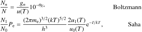 where N is the number of particles per unit volume, Nn is the fraction of atoms/ions excited to the nth state, gn is the statistical weight, θ = 5040 /T, T is the temperature, u(T) are the so-called partition functions, me is the electron mass, Pe is the electron pressure, and I is the ionization potential. More details can be found in e.g. Gray (2005). We note that the abundance determination are calculated through the MOOG code:
-
The effective temperature has a strong influence on thecorrelation of iron abundance with the excitation potential(excitation balance). We obtain the Teff when Fe i abundance shows no dependence on the excitation potential, i.e. the slope of abundance versus excitation potential is zero.
-
Surface gravity is derived from the ionization balance of Fe i and Fe ii abundances. Therefore, the abundance of neutral iron should be equal to the abundance of ionized iron and consistent with that of the input model atmosphere.
-
Microturbulence is connected with the saturation of the stronger iron lines. However, the abundances for weak and strong lines of a certain species (in our case iron) should be the same independent of the value of ξmicro. Iron abundances should show no dependence on the reduced EW (log (EW/λ)), i.e. the slope of abundance versus the reduced EW is zero.
Lastly, we change the input [Fe /H ] to match that of the average output [Fe /H ]. Hence we have four criteria to minimize simultaneously:
-
1.
The slope between abundance and excitation potential(aEP) has to be lower than 0.001.
-
2.
The slope between abundance and reduced EW (aRW) has to be lower than 0.003. We use 0.003 rather than 0.001 since this slope varies more rapidly with small changes in atmospheric parameters.
-
3.
The difference between the average abundances of Fe i and Fe ii (ΔFe ) should be less than 0.01.
-
4.
Input and output metallicity should be equal.
These criteria are used as indicators for the physical parameters we are trying to minimize. The constraints on the first three indicators are empirically defined.
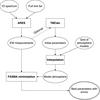 |
Fig. 1 General overview of FASMA from spectrum to parameters. |
There are many minimization routines available in Python. The ones from the SciPy ecosystem5 are the most commonly used. There are some advantages and disadvantages to using proprietary minimization routines. The advantages are that it is already written, and there is usually good documentation for libraries such as SciPy. The disadvantage in this situation is that most minimization routines do not work well with vector functions returning another vector: ![Mathematical equation: \begin{eqnarray} f(\{T_\mathrm{eff}, \log g, \textrm{[Fe/H]}, \xi_\mathrm{micro}\}) = \{a_\mathrm{EP}, a_\mathrm{RW}, \Delta\ion{Fe}, \ion{Fe}{I}\}. \label{eq:vector} \end{eqnarray}](/articles/aa/full_html/2017/04/aa29967-16/aa29967-16-eq21.png) (1)A workaround to this is to combine the criteria into one single criterion, for example by adding them quadratically and minimizing that expression instead. Thus, we have a vector function returning a scalar:
(1)A workaround to this is to combine the criteria into one single criterion, for example by adding them quadratically and minimizing that expression instead. Thus, we have a vector function returning a scalar: ![Mathematical equation: \begin{eqnarray} f(\{T_\mathrm{eff}, \log g, \textrm{[Fe/H]}, \xi_\mathrm{micro}\}) &= \sqrt{a_\mathrm{EP}^2 + a_\mathrm{RW}^2 + \Delta\ion{Fe}{}^2}. \label{eq:scalar} \end{eqnarray}](/articles/aa/full_html/2017/04/aa29967-16/aa29967-16-eq22.png) (2)The minimization routines are also not physical in the sense that they are not written for the problem. These two disadvantages encouraged us to write a specific minimization routine for the problem at hand. This also allowed us to minimize the more complicated expression in Eq. (1). Here is how it works:
(2)The minimization routines are also not physical in the sense that they are not written for the problem. These two disadvantages encouraged us to write a specific minimization routine for the problem at hand. This also allowed us to minimize the more complicated expression in Eq. (1). Here is how it works:
-
1.
Run MOOG once with user defined initial parameters (defaultis solar) and calculate aEP, aRW, and ΔFe .
-
2.
Change the atmospheric parameters (Teff, log g, [Fe /H ], ξmicro) according to the size of the indicator. A parameter is only changed if it is not fixed.
-
aEP: indicator for Teff. If this value is positive, then increase Teff. Decrease Teff if aEP is negative.
-
aRW: same as above, but for ξmicro.
-
ΔFe: positive ΔFe means log g should be decreased and vice versa.
-
[Fe /H] is changed to the output [Fe /H] in each iteration.
-
-
3.
If the new set of parameters have already been used in a previousiteration, then change them slightly. This is done by drawing arandom number from a Gaussian distribution with a mean at thecurrent value and a sigma equal to the absolute value of theindicator. For Teff the new value would be a random draw from
 and similar for the other atmospheric parameters using the appropriate indicators.
 -
4.
Calculate a new atmospheric model by interpolating a grid of models so we have the requested parameters and run MOOG once again.
-
5.
For each iteration save the parameters used and the quadratic sum of the indicators.
-
6.
Check for convergence, i.e. if the indicators are below or equal to the empirical constraints chosen. If we do not reach convergence, then return the best found parameters. The best found parameters, when convergence is not reached, are chosen when the quadratic sum of the indicators are smallest.
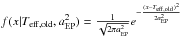
This whole process is shown schematically in Fig. 1, and the minimization routine itself in Fig. 2. By minimizing Eq. (1) rather than Eq. (2) we can reach convergence more quickly since we know in which direction we must change the atmospheric parameters. The stepping in parameters follows these simple empirical equations where we add the right side (sign change according to the sign of the indicator) to the left side: 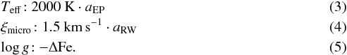 The metallicity is corrected at each step so the input metallicity matches that of the output metallicity of the previous iteration. The functional form (linear) for changing the parameters were found by changing one parameter, e.g. Teff, while keeping the other parameters fixed at their convergence values using the Sun as an example. A linear fit was applied to Teff−Teff,0 versus aEP in order to get the slope (2000 K for Teff). Since we ignore all interdependencies between the parameters, we slightly lowered the slopes found and arrived at the very simple equations above. By empirically determining how the atmospheric parameters should be changed in each iteration, we are able to swiftly approach the convergence value. The error estimates are based on the same method presented in Gonzalez & Laws (2000), which is also described in detail in Santos et al. (2003) and Andreasen et al. (2016).
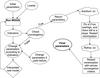 |
Fig. 2 Overview of the minimization for FASMA with the EW method. |
By using the indicators like this, we can reach convergence quickly. The typical calculation time for an FGK dwarf with a high-quality spectrum is around 2 min.
It is possible to run the EW method with a set of different options which are described here.
-
fixteff: this option fixes Teff and derives the other parameters. The same is available for log g (fixlogg), [Fe /H ] (fixfeh), and ξmicro (fixvt). One or more parameters can be fixed. When one or more parameters are fixed, the corresponding indicator will be ignored for each iteration, thus the parameter itself will not be changed.
-
outlier: remove a spectral line (or lines) after the minimization is done if the abundance of this spectral line is more than 3σ away from the average abundance of all the lines. After the removal of outlier(s) the minimization routine restarts. The options are to remove all outliers above 3σ once or iteratively, or to remove one outlier above 3σ once or iteratively.
-
autofixvt: if the minimization routine does not converge and ξmicro is close to 0 or 10 with a significant aRW (numerically bigger than 0.05), then fix ξmicro. This option was added since we saw this behaviour in some cases. The solution was typically to restart the minimization manually with ξmicro fixed. If ξmicro is fixed it is changed at each iteration according to an empirical relation. For dwarfs it follows the one presented in Tsantaki et al. (2013) and for giants it follows the one presented in Adibekyan et al. (2015b).
-
refine: after the minimization is done, run it again from the best found parameters but with stricter criteria. If this option is set, it will always be the last step (after removal of outliers). The convergence criteria can be changed by the user, but we recommend using the defaults provided above.
-
tmcalc: use TMCalc (Sousa et al. 2012) to quickly estimate the Teff and [Fe /H ] using the raw output from ARES. We then assume solar surface gravity (4.44 dex) and estimate ξmicro based on an empirical relation (see above).
For the optical we used the line list presented in Sousa et al. (2008). However, this line list does not work well for cool stars. This was fixed in Tsantaki et al. (2013) by removing some lines from Sousa et al. (2008). For stars cooler than 5200 K we automatically rederived the atmospheric parameters after removing lines so the line list resembled that of Tsantaki et al. (2013). The line list for the near-IR is also available (Andreasen et al. 2016).
All restarts of the minimization routine are done using the most recently found best parameters as initial conditions.
2.3. Abundance method
FASMA calculates element abundances for 12 different elements (Na , Mg , Al , Si , Ca , Ti , Cr , Ni , Co , Sc , Mn , and V ) from spectral lines determined in Neves et al. (2009) and Adibekyan et al. (2012). It also includes three ionized elements: Cr ii, Sc 2, and Ti ii. The abundances are derived using MOOG in the same way as described above for Fe . The atomic data were calibrated with the Sun as reference and solar abundances from Anders & Grevesse (1989). The EWs are measured automatically with the ARES driver of FASMA. The element abundance of each line is derived using the atmospheric parameters of the stars obtained from the previous step. The final element abundance is calculated from the weighted mean of the abundances produced by all lines detected for a given element as described in Adibekyan et al. (2015a).
2.4. Testing FASMA
To test the derivation of stellar parameters implemented in FASMA we derived parameters from the 582 sample by Sousa et al. (2011). We used ARES to measure the EWs. ARES can give an estimate of the S/N by analysing the continuum in certain intervals. For solar-type stars the following intervals worked well: 5764–5766 Å, 6047–6053 Å, and 6068–6076 Å. From the estimated S/N, ARES can give an estimate on the very important rejt parameters (see Sousa et al. 2015, for more information). After measuring the EWs with ARES, we used the FASMA minimization routine described in Sect. 2.2 to determine the stellar atmospheric parameters. The results are presented in Fig. 3 which shows Teff, log g, [Fe /H ], and ξmicro for FASMA against those of Sousa et al. (2011).
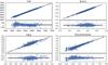 |
Fig. 3 Stellar atmospheric parameters derived by FASMA compared to the sample by Sousa et al. (2011). The x-axis in all plots shows the results from FASMA, while the y-axis shows the parameters derived by Sousa et al. (2011). |
The sample contains stars with Teff too cold for the line list used. As described in Sect. 2.2 we should then convert the line list by Sousa et al. (2008) to the line list presented in Tsantaki et al. (2013). However, since this line list was not available when Sousa et al. (2011) derived parameters, we did not make this change in order to make a fair comparison for FASMA.
The mean of the difference between parameters from Sousa et al. (2011) and those by FASMA are presented in Table 2.
Difference in derived parameters by Sousa et al. (2011) and FASMA.
The comparison is very consistent, as expected, and the small offsets are within the errors except for metallicity. This can be due to different versions of MOOG, measured line lists (i.e. using slightly different settings/version of ARES to measure the EWs), interpolation of atmosphere grid, and minimization routine. Most likely the difference will be due to the different rejt parameters used in ARES, which can alter the EWs systematically and hence the metallicity. We therefore randomly selected 20 stars with different Teff and used the EWs directly from Sousa et al. (2011) to derive parameters. The results are presented in the last column of Table 2. We note that the log gf values from the original line lists by Sousa et al. (2011), which used the MOOG 2002 version, were not changed for the 2014 version of MOOG. This might lead to some errors as well. However, the offsets are very small and are compatible with the errors on parameters normally obtained from high-quality spectra.
2.5. Web interface
We provide a web interface for FASMA. In the web interface it is possible to use the line list provided with FASMA to measure the EWs of a spectrum. The spectrum is expected to be in a 1D format with the wavelength information stored in the header keys, CRVAL1 for the minimum wavelength, CDELT1 for the stepping in wavelengths, and NAXIS1 for the number of points. This can be used for all the available FASMA methods described above. ARES does the normalization, but the best results are found when the spectrum is properly reduced (by removal of cosmic rays, normalization, etc.).
The web interface can be found online6, where more information is available on each of the drivers. The user must provide an email. This is only used to send the results after the calculations.
3. SWEET-Cat update
3.1. Data
In this paper we derived parameters for a sample of 50 stars, 43 were observed by our team using the UVES/VLT (Dekker et al. 2000), FEROS/2.2 m telescope in La Silla (Kaufer et al. 1999), and FIES/NOT (Frandsen & Lindberg 1999) spectrographs. The remaining spectra (23) were found in various archives. We use spectra from the HARPS/3.6 m telescope in La Silla (Mayor et al. 2003) and ESPaDOnS/CFHT (Donati 2003). Some characteristics of the spectrographs are presented in Table 3 with the mean S/N for the spectra used. The S/N for each star can be seen in Table A.1 along with the atmospheric parameters of the stars. The S/N is measured automatically by ARES, but we note that ARES smoothes the spectra before measuring the S/N, hence it is listed higher than the actual S/N. These 50 stars are confirmed exoplanet hosts listed in SWEET-Cat. However, they belonged to the list of stars that have not been analysed by our team. We therefore increase the number of stars analysed in a homogeneous way, which is the goal of SWEET-Cat.
We obtain the spectra with the highest possible resolution for a given spectrograph, and in cases with multiple observations, we include all the observations unless a spectrum is close to the saturation limit for a given spectrograph. For multiple spectra, we combine them after first correcting the radial velocity (RV) and using a sigma clipper to remove cosmic rays. The individual spectra are then combined to a single spectrum for a given star to increase the S/N. This single spectrum is used in the analysis described below. For most of the spectra in the archive included here, several spectra were combined as described above, while for the observations dedicated to this work, the spectrum would be a single spectrum, or in cases of faint stars, it would be observed a few times to reach the desired S/N. This is mostly due to the difference in science cases behind the observations; for example, the HARPS spectra were used for RV monitoring or follow-up of the exoplanet(s), while the UVES spectra were used to characterize stellar parameters.
Spectrographs used for this paper with their spectral resolution, wavelength coverage, and mean S/N from the spectra used.
3.2. Analysis
Here we present the sample of 50 stars. We were unable to derive parameters for 16 of our targets (not included in the 50). For example, HD 77065 is a spectroscopic binary according to Pourbaix et al. (2004), and the spectrum is contaminated by the companion star. This make EW measurement very difficult, hence we exclude it from the sample of collected spectra.
Moreover, we were not able to successfully derive parameters with this method for Aldebaran, a well-known red giant star. Even though spectra of good quality are available for a bright star like Aldebaran, this spectral type is intrinsically difficult to analyse, due to the molecular absorption that arises in the optical region at low Teff (4055 K is listed in SWEET-Cat as measured by Hatzes et al. 2015). The fact that we are not able to derive parameters for Aldebaran is not a big concern since it has been well studied with other techniques, and we can trust the parameters already listed in SWEET-Cat.
In total, we removed 16 stars from our sample because the parameters for these stars did not converge during the minimization procedure. The Teff for these stars is either too hot, above 7500 K, or too cold, below 4000 K, for the EW method to work.
The remaining 50 stars are presented in Table A.1. We note that we apply a correction to the spectroscopic log g based on asteroseismology as found by Mortier et al. (2014). We only use this correction for FGK dwarf stars, i.e. between 4800 K≤ Teff ≤6500 K and log g ≥ 4.2. For stars with a log g lower than this limit we do not apply the corrections, and if the log g changes to below this limit after the correction, we go back to using the spectroscopic log g again. The correction for log g depends on both Teff and log g. The correction can be up to 0.5 dex, depending on the Teff.
We present a Hertzprung-Russel diagram (HRD) of our sample in Fig. 4, which is made with a tool for post-processing the results saved to a table by FASMA.
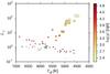 |
Fig. 4 Hertzprung-Russel diagram of our sample with the Sun as a green star. The size of the points represents the log g, with bigger points being smaller log g (giants), and vice versa. Red points are the dwarfs, while yellow points are the giants. |
The new atmospheric parameters are presented in Fig. 5 against the literature values that we listed previously in SWEET-Cat. The red points showing the location of the outliers as discussed below are mainly visible outliers for log g at the low end, i.e. for the sub-giant to giant stars. The old parameters are listed in Table A.2. Out of 2437 stars discovered to be a planet hosts, 21% have been analysed in the homogeneous way as described in this work. We note that currently the limiting factor for increasing the sample of stars analysed in the homogeneous way is the magnitude of the planet hosts. Many planet hosts have been found through space missions such as Kepler and CoRoT using the transiting method. Most of these stars are faint and thus make them observationally expensive for the spectroscopic analysis required here. For stars brighter than magnitude 12 the completeness (i.e. the stars analysed in a homogeneous way compared to the ones we have not analysed yet) is now up to 77%, while it is at 85% for exoplanet hosts brighter than magnitude 10.
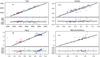 |
Fig. 5 Atmospheric parameters of the updated planet host stars. The x-axis shows the previous values in SWEET-Cat (see Table A.2), while the y-axis indicates the new updated values. In the upper left corner of each of the four plots we show the typical error on the parameters. The red points are outliers, as discussed in Sect. 3.3. |
Understanding the metallicity distribution for all the planet host stars is important in order to understand planet formation, for example. We present a distribution in Fig. 6. The sample is divided in two, for all planet hosts in SWEET-Cat and for stars brighter than 12 V magnitude. Dimmer stars are mainly observed with the Kepler space mission. These dim stars are very time consuming, and hence expensive to observe. Out of the 2437 stars in SWEET-Cat, 664 are brighter than 12 V magnitude. We note that more than 1500 of the stars do not have a V magnitude. The majority are stars observed with Kepler. Our group have analysed 563 stars in SWEET-Cat including the 50 stars presented in this work.
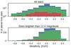 |
Fig. 6 Metallicity distribution. Top: all stars (logarithmic scale) in SWEET-Cat, divided in three groups: blue (the largest distribution) are all stars available in SWEET-Cat; green (the middle distribution) are the stars with homogeneity flag 1, i.e. analysed using the method described in this paper; and red (the smallest distribution) are all new stars added from this paper. Bottom: 12 V magnitude cut to exclude stars which are currently unavailable spectroscopically. |
3.3. Discussion
We compute radius and mass of all the 50 new stars updated in SWEET-Cat (even the ones whose parameters may not be reliable, in order to be complete) using the empirical formula presented in Torres et al. (2010). Some of the stars have radii derived from different methods, usually from isochrones. These radii generally show a good correlation with radii derived from Torres et al. (2010) if the literature parameters of Teff, log g, and [ Fe / H ] are used. However, if we make a comparison with the new radius derived using the parameters presented here, the results can differ by up to 65%. We show in Fig. 7 how the radius calculated from Torres et al. (2010) differs between the literature atmospheric parameters and the new homogeneous atmospheric parameters presented here. We note that stellar radii are provided by many of the authors from different discovery papers, but we chose to compare the atmospheric parameters via the derivation of the stellar radius, as described above, rather than comparing the stellar radii from different methods.
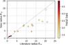 |
Fig. 7 Stellar radius on both axes calculated based on Torres et al. (2010). The x-axis shows the stellar radius based on the atmospheric parameters from the literature, while the y-axis indicates the new homogeneous parameters presented here. The colour and size indicate the surface gravity. This clearly shows that the disagreement is biggest for more evolved stars. |
In the sections below we discuss the systems (seven stars, eight exoplanets) where the radius or mass of the stars changes more than 25% and how this influences the planetary parameters. The changes in radius for a star is primarily due to changes in log g, which can be used as an indicator of the evolutionary stage of a star.
We rederive the planetary radius, mass, and semi-major axis when possible following the three simple scaling relations based on Newton’s law of gravity (Newton 1687) for deriving mass and distance and simple geometry for radius (see e.g. Torres et al. 2008) 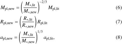 where the subscript “lit” denotes the value from the literature used in the comparison, the subscript “new” indicates the new computed values, the subscript “pl” is short for planet, and the subscript “∗” is short for star; M, R, and a are mass, radius, and semi-major axis, respectively. We note that for the literature values, we use the values reported directly from the literature and not the derived radius and mass from Torres et al. (2010). To identify outliers, we compare radii and masses derived from Torres et al. (2010) since this is a measure of how the atmospheric parameters have changed.
3.3.1. HAT-P-46
HAT-P-46 has two known exoplanets according to Hartman et al. (2014a). The outer planet HAT-P-46 c is not transiting, hence we do not have a radius for this planet. The results we present in this paper for this star come from UVES/VLT data with a S/N of 208. Hartman et al. (2014a) derives the following spectroscopic parameters: Teff =6120(100) K, log g = 4.25 ± 0.11, and [Fe /H ] = 0.30 ± 0.10. We note that for this star the asteroseismic correction we apply (see Sect. 3.2) results in a corrected log g below 4.2 dex, so we used the spectroscopic log g for this star.
If we derive the mass and radius of HAT-P-46 b with our new parameters, we obtain Rpl = 0.93 RJ, while Hartman et al. (2014a) derived Rpl = 1.28 RJ. We see no change in mass (Hartman et al. 2014a found Mpl = 0.49 MJ); however, there is a decrease in the radius, and we end up with a more dense planet, ρpl =0.76 g/cm3 from ρpl = 0.28 ± 0.10 g/cm3.
As the secondary companion does not transit we only have a limit on the minimum mass for this planet. Here we get Msinipl = 1.97 MJ and Hartman et al. (2014a) presented Msinipl = 2.00 MJ, so a very small change, as expected.
3.3.2. HD 120084
The exoplanet orbiting this star with a period of 2082 days and a quite eccentric orbit at 0.66 was discovered by Sato et al. (2013a). The atmospheric parameters were derived by Takeda et al. (2008) using a similar method to that described in this paper. The quality of the spectra they analysed, however, were not as high as those used here. Using the HIDES spectrograph at the 188 cm reflector at NAOJ, Takeda et al. (2008) reported an average S/N for their sample of 100–300 objects at a resolving power of 67 000. We used data from ESPaDOnS with a resolving power of 81 000, and with a S/N for this star of 850. With our new parameters we obtain a slightly lower stellar mass for the star at 1.93 M⊙ compared to 2.39 M⊙ obtained by Takeda et al. (2008), hence the minimum planetary mass is also slightly lower, from mplsini = 4.5 MJ to mplsini = 3.9 MJ. We see a 28% decrease in the stellar radius, from 9.12 R⊙ to 7.81 R⊙. Since there are no observations of the planet transiting, the planetary radius has not been computed.
3.3.3. HD 233604
HD 233604 b was discovered by Nowak et al. (2013), while the atmospheric parameters of the star were derived by Zieliński et al. (2012), who used the same method as described in this paper using the HRS spectrograph at HET with a resolving power of 60 000 with a typical S/N at 200–250. We obtained the spectrum for this star using the FIES spectrograph with a slightly higher resolution at 67 000, and similar but also slightly higher S/N at 320 for this star.
This planet is in a very close orbit with a semi-major axis of ~15 R∗ (R∗ is the stellar radius) using the parameters from Nowak et al. (2013). Using the updated parameters presented in this paper we see a slight increase in the stellar mass from 1.5 M⊙ to 1.9 M⊙, and a decrease in stellar radius from 10.5 R⊙ to 8.6 R⊙. This increases the semi-major axis to ~21 R∗. We note that the correct stellar radii are used to describe the semi-major axis in both cases. The increase in stellar mass leads to an increase in the minimum planetary mass, from mplsini = 6.58 MJ to mplsini = 7.79 MJ.
Nowak et al. (2013) found a high Li abundance at A(Li )LTE = 1.400 ± 0.042 for this star and speculated that this star might have engulfed a planet. A more likely explanation is that this star has not yet reached the first dredge-up process (Nowak et al. 2013). We found a much lower value, A(Li )LTE = 0.92, and hence do not find the star to be Li rich. The Li abundance we find is in excellent agreement with Adamów et al. (2014). Even applying a NLTE correction, as was done in Adamów et al. (2014) (A(Li )NLTE = 1.08), this star is not Li rich.
3.3.4. HD 5583
This exoplanet was discovered by Niedzielski et al. (2016) with an orbital period of 139 days around a K giant. This exoplanet was discovered with the radial velocity technique, and we do not have a planetary radius. The stellar parameters were derived in a similar manner to that presented here (see Niedzielski et al. 2016, and references therein); our biggest disagreement is in the surface gravity. We derive a log g that is higher by 0.34 dex, which gives a stellar radius that is smaller by 37%. The derived mass is 15% higher, which in turn increases the minimum planetary mass from mplsini = 5.78 MJ to mplsini = 8.63 MJ. Even with the increase in mass, it is still within the planetary regime for most inclinations, as was noted by Niedzielski et al. (2016).
3.3.5. HD 81688
This exoplanet was discovered by Sato et al. (2008) with the RV method. The host star is a metal-poor K giant. The atmospheric parameters presented in Sato et al. (2008) are obtained via the same method as presented in this paper, and the agreement is quite good. Once again the big disagreement is in the surface gravity: ours is 0.48 dex higher. Even though the stellar parameters, and hence the planetary parameters, do change, the radius and mass we derive are not far from the values presented in the paper by Sato et al. (2008). This is a case where the star was marked as an outlier, due to the comparison between the radius and mass derived from Torres et al. (2010).
The new stellar mass is the same as before, 2.1 M⊙. The stellar radius changed from 13.0 R⊙ to 10.8 R⊙. Since a transit of this star has not been observed and the stellar mass remains the same, we do not see any change in the planetary parameters.
We note that this system is in an interesting configuration with a very close orbit around an evolved star. This system, among others, has been the subject of work on planet engulfment (see e.g. Kunitomo et al. 2011).
3.3.6. HIP 107773
The planetary companion was presented in Jones et al. (2015) as an exoplanet around an intermediate-mass evolved star. The stellar parameters were obtained from the analysis by Jones et al. (2011) using the same method as presented here, but with a different line list, which might lead to some disagreements. For this star we derive a higher log g (2.83 dex compared to 2.60 dex), thus we derive a slightly smaller star with 11.6 R⊙ to 9.2 R⊙ and 2.4 M⊙ to 2.1 M⊙ for radius and mass of the star, respectively. The other atmospheric parameters are very similar to those derived by Jones et al. (2011). This leads to a reduced minimum mass of the planetary companion from msini = 1.98 MJ to msini = 1.78 MJ. The planetary radius has not been measured.
3.3.7. WASP-97
The exoplanet orbiting WASP-97 was discovered by Hellier et al. (2014). The host star parameters were derived using a similar method to that described in this paper after co-adding several spectra from the CORALIE spectrograph. They reach a S/N of 100 with a spectral resolution of 50 000. The parameters presented here come from the UVES spectrograph with a S/N of more than 200.
The parameters do not change much for this planet. The planetary mass changes from mplsini = 1.32 MJ to mplsini = 1.37 MJ and the radius from 1.13 RJ to 1.42 RJ. This affects the density quite strongly; it changes from 1.13 g/cm3 to 0.59 g/cm3. This exoplanet is then in the same category as Saturn; its density is lower than water, but it is slightly larger than Jupiter.
3.3.8. ω Serpentis (ome Ser)
The exoplanet orbiting this star with a period of 277 days and an eccentric orbit at 0.11 was also presented by Sato et al. (2013a). The atmospheric parameters were derived in the same way as for HD 120084. We used data from FIES with a resolving power of 67 000, and with a S/N for this star of 1168. With our new parameters we obtain a slightly higher stellar mass for the star at 2.19 M⊙ compared to the value of 2.17 M⊙ obtained by Takeda et al. (2008). This change is not significant enough to change the minimum planetary mass at mplsini = 1.7 MJ. The stellar radius decreases by more than one solar radius, from 12.3 R⊙ to 11.1 R⊙. However, since there are no observations of transiting exoplanets, we cannot see the change in the planetary radius.
3.3.9. o Ursa Major (omi UMa)
omi UMa b was discovered by Sato et al. (2012) using the RV method. The stellar parameters are from Takeda et al. (2008), as discussed above. The spectrum used for this star is from ESPaDOnS with a S/N of more than 500 compared to the value of 100–300 reached for the large sample presented in Takeda et al. (2008). The luminosity and mass for omi UMa were obtained from theoretical evolutionary tracks (see Sato et al. 2012, and references therein). The radius was then estimated using the Stefan-Boltzmann relationship, using the measured luminosity and Teff.
The parameters presented here mainly differ in the surface gravity: ours is 0.72 dex higher at log g = 3.36. This leads to a big change in stellar mass and radius from 3.1 M⊙ to 1.6 M⊙ and 14.1 R⊙ to 4.5 R⊙, respectively. Sato et al. (2012) have reported that omi UMa b is the first planet candidate around a star more massive than 3 M⊙. With these updated results, the minimum mass of the planet is now msini = 2.7 MJ, whereas previously it was msini = 4.1 MJ (Sato et al. 2012). The exoplanet is not reported to transit, as seen from Earth, so we do not have a radius for this exoplanet, which would have changed a great deal with these new results.
4. Conclusion
With this update we bring the completeness of SWEET-Cat for stars brighter than magnitude 10 (V band) up to 85% (77% for stars brighter than 12). The parameters are continuously updated and are available for the public in an easily accessibly form7. The importance of the homogeneous analysis which we keep striving for is shown in Fig. 7 where we see quite different derived stellar radii when the atmospheric parameters are obtained via different methods. Even using the same method but with a different setup (different line list, minimization routine, atmospheric models, etc.), we can arrive at different results. This again shows the importance of analysing the stars in a homogeneous way. As has been discussed in Sect. 3.3 this has a direct impact on the planetary parameters. It is of great importance to know the planetary parameters very well, for individual systems and also for an ensemble. With accurate and precise planetary parameters we will be able to distinguish the different possible compositions, whether gas giants, water worlds, or rocky planets.
Finally we also provide an online tool for deriving the stellar atmospheric parameters using FASMA. We recommend this tool only for spectra and stars where this method is working, i.e. high-resolution spectra with a high S/N. The stars can be FGK dwarfs and FGK subgiants/giants. We are working on applying this method to the near-IR in order to include the cool solar-type stars.
For an updated table we refer to http://www.exoplanet.eu
ARES, in principle, just needs a list of wavelengths in order to run, but is often used with a line list with characteristics of the atomic absorption line.
Acknowledgments
This work was supported by Fundação para a Ciência e a Tecnologia (FCT) through national funds and by FEDER through COMPETE2020 by these grants UID/FIS/0Q4434/2013 & POCI-01-0145-FEDER-007672, PTDC/FIS-AST/7073/2014 & POCI-01-0145-FEDER-016880 and PTDC/FIS-AST/1526/2014 & POCI-01-0145-FEDER-016886. S.G.S. and N.C.S. acknowledge the support from FCT through the Investigador FCT Contracts of reference IF/00028/2014/CP1215/CT0002 and IF/00169/2012/CP0150/CT0002, respectively, and POPH/FSE (EC) by FEDER funding through the program “Programa Operacional de Factores de Competitividade – COMPETE”. G.D.C.T. was supported by the PhD fellowship PD/BD/113478/2015funded by FCT (Portugal) and POPH/FSE (EC). E.D.M. acknowledge the support by the fellowship SFRH/BPD/76606/2011funded by FCT (Portugal) and POPH/FSE (EC). A.C.S.F. was supported by grant 234989/2014-9 from CNPq (Brazil). A.M. received funding from the European Union Seventh Framework Programme (FP7/2007–2013) under grant agreement number 313014 (ETAEARTH). This research has made use of the SIMBAD database operated at CDS, Strasbourg (France). We thank the anonymous referee for the useful comments and suggestions which helped clarify the manuscript.
References
- Adamów, M., Niedzielski, A., Villaver, E., Wolszczan, A., & Nowak, G. 2014, A&A, 569, A55 [NASA ADS] [CrossRef] [EDP Sciences] [Google Scholar]
- Adibekyan, V. Z., Sousa, S. G., Santos, N. C., et al. 2012, A&A, 545, A32 [NASA ADS] [CrossRef] [EDP Sciences] [Google Scholar]
- Adibekyan, V., Figueira, P., Santos, N. C., et al. 2015a, A&A, 583, A94 [NASA ADS] [CrossRef] [EDP Sciences] [Google Scholar]
- Adibekyan, V. Z., Benamati, L., Santos, N. C., et al. 2015b, MNRAS, 450, 1900 [NASA ADS] [CrossRef] [Google Scholar]
- Anders, E., & Grevesse, N. 1989, Geochim. Cosmochim. Acta, 53, 197 [Google Scholar]
- Anderson, D. R., Collier Cameron, A., Gillon, M., et al. 2012, MNRAS, 422, 1988 [NASA ADS] [CrossRef] [Google Scholar]
- Andreasen, D. T., Sousa, S. G., Delgado Mena, E., et al. 2016, A&A, 585, A143 [NASA ADS] [CrossRef] [EDP Sciences] [Google Scholar]
- Barclay, T., Rowe, J. F., Lissauer, J. J., et al. 2013, Nature, 494, 452 [NASA ADS] [CrossRef] [Google Scholar]
- Bedell, M., Meléndez, J., Bean, J. L., et al. 2015, A&A, 581, A34 [NASA ADS] [CrossRef] [EDP Sciences] [Google Scholar]
- Boisse, I., Hartman, J. D., Bakos, G. Á., et al. 2013, A&A, 558, A86 [NASA ADS] [CrossRef] [EDP Sciences] [Google Scholar]
- Brucalassi, A., Pasquini, L., Saglia, R., et al. 2014, A&A, 561, L9 [NASA ADS] [CrossRef] [EDP Sciences] [Google Scholar]
- Bryan, M. L., Alsubai, K. A., Latham, D. W., et al. 2012, ApJ, 750, 84 [NASA ADS] [CrossRef] [Google Scholar]
- Campante, T. L., Barclay, T., Swift, J. J., et al. 2015, ApJ, 799, 170 [NASA ADS] [CrossRef] [Google Scholar]
- Collins, K. A., Eastman, J. D., Beatty, T. G., et al. 2014, AJ, 147, 39 [NASA ADS] [CrossRef] [Google Scholar]
- Dekker, H., D’Odorico, S., Kaufer, A., Delabre, B., & Kotzlowski, H. 2000, in Optical and IR Telescope Instrumentation and Detectors, eds. M. Iye, & A. F. Moorwood, Proc. SPIE, 4008, 534 [Google Scholar]
- Delrez, L., Van Grootel, V., Anderson, D. R., et al. 2014, A&A, 563, A143 [NASA ADS] [CrossRef] [EDP Sciences] [Google Scholar]
- Donati, J.-F. 2003, in Solar Polarization, eds. J. Trujillo-Bueno, & J. Sanchez Almeida, ASP Conf. Ser., 307, 41 [Google Scholar]
- Frandsen, S., & Lindberg, B. 1999, in Astrophysics with the NOT, eds. H. Karttunen, & V. Piirola, 71 [Google Scholar]
- Gillon, M., Anderson, D. R., Collier-Cameron, A., et al. 2013, A&A, 552, A82 [NASA ADS] [CrossRef] [EDP Sciences] [Google Scholar]
- Gómez Maqueo Chew, Y., Faedi, F., Pollacco, D., et al. 2013, A&A, 559, A36 [NASA ADS] [CrossRef] [EDP Sciences] [Google Scholar]
- Gonzalez, G., & Laws, C. 2000, AJ, 119, 390 [NASA ADS] [CrossRef] [Google Scholar]
- Gray, D. F. 2005, The Observation and Analysis of Stellar Photospheres, 3rd ed. (Cambridge: Cambridge University Press) [Google Scholar]
- Gustafsson, B., Edvardsson, B., Eriksson, K., et al. 2008, A&A, 486, 951 [NASA ADS] [CrossRef] [EDP Sciences] [Google Scholar]
- Hartman, J. D., Bakos, G. Á., Béky, B., et al. 2012, AJ, 144, 139 [NASA ADS] [CrossRef] [Google Scholar]
- Hartman, J. D., Bakos, G. Á., Torres, G., et al. 2014a, AJ, 147, 128 [NASA ADS] [CrossRef] [Google Scholar]
- Hartman, J. D., Bakos, G. Á., Torres, G., et al. 2014b, AJ, 147, 128 [NASA ADS] [CrossRef] [Google Scholar]
- Hatzes, A. P., Cochran, W. D., Endl, M., et al. 2015, A&A, 580, A31 [NASA ADS] [CrossRef] [EDP Sciences] [Google Scholar]
- Hébrard, G., Collier Cameron, A., Brown, D. J. A., et al. 2013, A&A, 549, A134 [NASA ADS] [CrossRef] [EDP Sciences] [Google Scholar]
- Hébrard, G., Arnold, L., Forveille, T., et al. 2016, A&A, 588, A145 [NASA ADS] [CrossRef] [EDP Sciences] [Google Scholar]
- Hellier, C., Anderson, D. R., Collier Cameron, A., et al. 2012, MNRAS, 426, 739 [NASA ADS] [CrossRef] [Google Scholar]
- Hellier, C., Anderson, D. R., Cameron, A. C., et al. 2014, MNRAS, 440, 1982 [NASA ADS] [CrossRef] [Google Scholar]
- Howard, A. W., Johnson, J. A., Marcy, G. W., et al. 2011, ApJ, 730, 10 [NASA ADS] [CrossRef] [Google Scholar]
- Johnson, J. A., Clanton, C., Howard, A. W., et al. 2011, ApJS, 197, 26 [NASA ADS] [CrossRef] [Google Scholar]
- Jones, M. I., Jenkins, J. S., Rojo, P., & Melo, C. H. F. 2011, A&A, 536, A71 [NASA ADS] [CrossRef] [EDP Sciences] [Google Scholar]
- Jones, M. I., Jenkins, J. S., Rojo, P., Olivares, F., & Melo, C. H. F. 2015, A&A, 580, A14 [NASA ADS] [CrossRef] [EDP Sciences] [Google Scholar]
- Kaufer, A., Stahl, O., Tubbesing, S., et al. 1999, The Messenger, 95, 8 [Google Scholar]
- Kipping, D. M., Bakos, G. Á., Hartman, J., et al. 2010, ApJ, 725, 2017 [NASA ADS] [CrossRef] [Google Scholar]
- Kunitomo, M., Ikoma, M., Sato, B., Katsuta, Y., & Ida, S. 2011, ApJ, 737, 66 [NASA ADS] [CrossRef] [Google Scholar]
- Kurucz, R. 1993, ATLAS9 Stellar Atmosphere Programs and 2 km s-1 grid. Kurucz CD-ROM No. 13. (Cambridge, Mass.: Smithsonian Astrophysical Observatory) [Google Scholar]
- Lee, B.-C., Han, I., & Park, M.-G. 2013, A&A, 549, A2 [NASA ADS] [CrossRef] [EDP Sciences] [Google Scholar]
- Lee, B.-C., Han, I., Park, M.-G., et al. 2014, A&A, 566, A67 [NASA ADS] [CrossRef] [EDP Sciences] [Google Scholar]
- Mayor, M., Pepe, F., Queloz, D., et al. 2003, The Messenger, 114, 20 [NASA ADS] [Google Scholar]
- Mészáros, S., Allen de Prieto, C., Edvardsson, B., et al. 2012, AJ, 144, 120 [NASA ADS] [CrossRef] [Google Scholar]
- Mortier, A., Santos, N. C., Sousa, S., et al. 2013, A&A, 551, A112 [NASA ADS] [CrossRef] [EDP Sciences] [Google Scholar]
- Mortier, A., Sousa, S. G., Adibekyan, V. Z., Brandão, I. M., & Santos, N. C. 2014, A&A, 572, A95 [NASA ADS] [CrossRef] [EDP Sciences] [Google Scholar]
- Motalebi, F., Udry, S., Gillon, M., et al. 2015, A&A, 584, A72 [NASA ADS] [CrossRef] [EDP Sciences] [Google Scholar]
- Moutou, C., Lo Curto, G., Mayor, M., et al. 2015, A&A, 576, A48 [NASA ADS] [CrossRef] [EDP Sciences] [Google Scholar]
- Neves, V., Santos, N. C., Sousa, S. G., Correia, A. C. M., & Israelian, G. 2009, A&A, 497, 563 [NASA ADS] [CrossRef] [EDP Sciences] [Google Scholar]
- Neveu-VanMalle, M., Queloz, D., Anderson, D. R., et al. 2014, A&A, 572, A49 [NASA ADS] [CrossRef] [EDP Sciences] [Google Scholar]
- Newton, I. 1687, Philosophiae Naturalis Principia Mathematica. Auctore Js. Newton [Google Scholar]
- Niedzielski, A., Villaver, E., Wolszczan, A., et al. 2015a, A&A, 573, A36 [NASA ADS] [CrossRef] [EDP Sciences] [Google Scholar]
- Niedzielski, A., Wolszczan, A., Nowak, G., et al. 2015b, ApJ, 803, 1 [Google Scholar]
- Niedzielski, A., Villaver, E., Nowak, G., et al. 2016, A&A, 588, A62 [NASA ADS] [CrossRef] [EDP Sciences] [Google Scholar]
- Nowak, G., Niedzielski, A., Wolszczan, A., Adamów, M., & Maciejewski, G. 2013, ApJ, 770, 53 [Google Scholar]
- Penev, K., Bakos, G. Á., Bayliss, D., et al. 2013, AJ, 145, 5 [NASA ADS] [CrossRef] [Google Scholar]
- Pourbaix, D., Tokovinin, A. A., Batten, A. H., et al. 2004, A&A, 424, 727 [NASA ADS] [CrossRef] [EDP Sciences] [Google Scholar]
- Quinn, S. N., White, R. J., Latham, D. W., et al. 2014, ApJ, 787, 27 [NASA ADS] [CrossRef] [Google Scholar]
- Santos, N. C., Israelian, G., Mayor, M., Rebolo, R., & Udry, S. 2003, A&A, 398, 363 [NASA ADS] [CrossRef] [EDP Sciences] [Google Scholar]
- Santos, N. C., Sousa, S. G., Mortier, A., et al. 2013, A&A, 556, A150 [NASA ADS] [CrossRef] [EDP Sciences] [Google Scholar]
- Sato, B., Izumiura, H., Toyota, E., et al. 2008, PASJ, 60, 539 [NASA ADS] [Google Scholar]
- Sato, B., Omiya, M., Harakawa, H., et al. 2012, PASJ, 64, 135 [NASA ADS] [CrossRef] [Google Scholar]
- Sato, B., Omiya, M., Harakawa, H., et al. 2013a, PASJ, 65, 85 [NASA ADS] [Google Scholar]
- Sato, B., Omiya, M., Wittenmyer, R. A., et al. 2013b, ApJ, 762, 9 [NASA ADS] [CrossRef] [Google Scholar]
- Simpson, E. K., Faedi, F., Barros, S. C. C., et al. 2011, AJ, 141, 8 [NASA ADS] [CrossRef] [Google Scholar]
- Sneden, C. A. 1973, Ph.D. Thesis, The University of Texas at Austin [Google Scholar]
- Sousa, S. G., Santos, N. C., Israelian, G., Mayor, M., & Monteiro, M. J. P. F. G. 2007, A&A, 469, 783 [NASA ADS] [CrossRef] [EDP Sciences] [Google Scholar]
- Sousa, S. G., Santos, N. C., Mayor, M., et al. 2008, A&A, 487, 373 [NASA ADS] [CrossRef] [EDP Sciences] [MathSciNet] [Google Scholar]
- Sousa, S. G., Santos, N. C., Israelian, G., Mayor, M., & Udry, S. 2011, A&A, 533, A141 [NASA ADS] [CrossRef] [EDP Sciences] [Google Scholar]
- Sousa, S. G., Santos, N. C., & Israelian, G. 2012, A&A, 544, A122 [NASA ADS] [CrossRef] [EDP Sciences] [Google Scholar]
- Sousa, S. G., Santos, N. C., Adibekyan, V., Delgado-Mena, E., & Israelian, G. 2015, A&A, 577, A67 [NASA ADS] [CrossRef] [EDP Sciences] [Google Scholar]
- Takeda, Y., Sato, B., & Murata, D. 2008, PASJ, 60, 781 [NASA ADS] [CrossRef] [Google Scholar]
- Torres, G., Winn, J. N., & Holman, M. J. 2008, ApJ, 677, 1324 [NASA ADS] [CrossRef] [Google Scholar]
- Torres, G., Andersen, J., & Giménez, A. 2010, A&ARv, 18, 67 [Google Scholar]
- Torres, G., Fischer, D. A., Sozzetti, A., et al. 2012, ApJ, 757, 161 [NASA ADS] [CrossRef] [Google Scholar]
- Tsantaki, M., Sousa, S. G., Adibekyan, V. Z., et al. 2013, A&A, 555, A150 [NASA ADS] [CrossRef] [EDP Sciences] [Google Scholar]
- Valenti, J. A., & Fischer, D. A. 2005, ApJS, 159, 141 [NASA ADS] [CrossRef] [MathSciNet] [Google Scholar]
- Vanderburg, A., Montet, B. T., Johnson, J. A., et al. 2015, ApJ, 800, 59 [NASA ADS] [CrossRef] [Google Scholar]
- West, R. G., Hellier, C., Almenara, J.-M., et al. 2016, A&A, 585, A126 [NASA ADS] [CrossRef] [EDP Sciences] [Google Scholar]
- Wilson, P. A., Hébrard, G., Santos, N. C., et al. 2016, A&A, 588, A144 [NASA ADS] [CrossRef] [EDP Sciences] [Google Scholar]
- Zhou, G., Bayliss, D., Penev, K., et al. 2014, AJ, 147, 144 [NASA ADS] [CrossRef] [Google Scholar]
- Zieliński, P., Niedzielski, A., Wolszczan, A., Adamów, M., & Nowak, G. 2012, A&A, 547, A91 [NASA ADS] [CrossRef] [EDP Sciences] [Google Scholar]
Appendix A: Updated parameters of 50 planet hosts
Derived parameters for the 50 stars in our sample.
Previous parameters from SWEET-Cat.
All Tables
Spectrographs used for this paper with their spectral resolution, wavelength coverage, and mean S/N from the spectra used.
All Figures
|
Fig. 1 General overview of FASMA from spectrum to parameters. |
| In the text | |
|
Fig. 2 Overview of the minimization for FASMA with the EW method. |
| In the text | |
|
Fig. 3 Stellar atmospheric parameters derived by FASMA compared to the sample by Sousa et al. (2011). The x-axis in all plots shows the results from FASMA, while the y-axis shows the parameters derived by Sousa et al. (2011). |
| In the text | |
|
Fig. 4 Hertzprung-Russel diagram of our sample with the Sun as a green star. The size of the points represents the log g, with bigger points being smaller log g (giants), and vice versa. Red points are the dwarfs, while yellow points are the giants. |
| In the text | |
|
Fig. 5 Atmospheric parameters of the updated planet host stars. The x-axis shows the previous values in SWEET-Cat (see Table A.2), while the y-axis indicates the new updated values. In the upper left corner of each of the four plots we show the typical error on the parameters. The red points are outliers, as discussed in Sect. 3.3. |
| In the text | |
|
Fig. 6 Metallicity distribution. Top: all stars (logarithmic scale) in SWEET-Cat, divided in three groups: blue (the largest distribution) are all stars available in SWEET-Cat; green (the middle distribution) are the stars with homogeneity flag 1, i.e. analysed using the method described in this paper; and red (the smallest distribution) are all new stars added from this paper. Bottom: 12 V magnitude cut to exclude stars which are currently unavailable spectroscopically. |
| In the text | |
|
Fig. 7 Stellar radius on both axes calculated based on Torres et al. (2010). The x-axis shows the stellar radius based on the atmospheric parameters from the literature, while the y-axis indicates the new homogeneous parameters presented here. The colour and size indicate the surface gravity. This clearly shows that the disagreement is biggest for more evolved stars. |
| In the text | |
Current usage metrics show cumulative count of Article Views (full-text article views including HTML views, PDF and ePub downloads, according to the available data) and Abstracts Views on Vision4Press platform.
Data correspond to usage on the plateform after 2015. The current usage metrics is available 48-96 hours after online publication and is updated daily on week days.
Initial download of the metrics may take a while.