| Issue |
A&A
Volume 600, April 2017
|
|
|---|---|---|
| Article Number | A97 | |
| Number of page(s) | 15 | |
| Section | Extragalactic astronomy | |
| DOI | https://doi.org/10.1051/0004-6361/201526433 | |
| Published online | 06 April 2017 | |
Probing the radio loud/quiet AGN dichotomy with quasar clustering
Leiden Observatory, Leiden University, PO Box 9513, 2300 RA Leiden, The Netherlands
e-mail: This email address is being protected from spambots. You need JavaScript enabled to view it.
Received: 28 April 2015
Accepted: 2 November 2016
Abstract
We investigate the clustering properties of 45 441 radio-quiet quasars (RQQs) and 3493 radio-loud quasars (RLQs) drawn from a joint use of the Sloan Digital Sky Survey (SDSS) and Faint Images of the Radio Sky at 20 cm (FIRST) surveys in the range 0.3 < z < 2.3. This large spectroscopic quasar sample allow us to investigate the clustering signal dependence on radio-loudness and black hole (BH) virial mass. We find that RLQs are clustered more strongly than RQQs in all the redshift bins considered. We find a real-space correlation length of r0 = 6.59-0.24+0.33 h-1 Mpc and r0 = 10.95-1.58+1.22 h-1 Mpc for RQQs and RLQs, respectively, for the full redshift range. This implies that RLQs are found in more massive host haloes than RQQs in our samples, with mean host halo masses of ~ 4.9 × 10¹³h-1M⊙ and ~ 1.9 × 10¹²h-1M⊙, respectively. Comparison with clustering studies of different radio source samples indicates that this mass scale of ≳ 1 × 10¹³h-1M⊙ is characteristic for the bright radio-population, which corresponds to the typical mass of galaxy groups and galaxy clusters. The similarity we find in correlation lengths and host halo masses for RLQs, radio galaxies and flat-spectrum radio quasars agrees with orientation-driven unification models. Additionally, the clustering signal shows a dependence on BH mass, with the quasars powered by the most massive BHs clustering more strongly than quasars having less massive BHs. We suggest that the current virial BH mass estimates may be a valid BH proxies for studying quasar clustering. We compare our results to a previous theoretical model that assumes that quasar activity is driven by cold accretion via mergers of gas-rich galaxies. While the model can explain the bias and halo masses for RQQs, it cannot reproduce the higher bias and host halo masses for RLQs. We argue that other BH properties such as BH spin, environment, magnetic field configuration, and accretion physics must be considered to fully understand the origin of radio-emission in quasars and its relation to the higher clustering.
Key words: quasars: general / quasars: supermassive black holes / radio continuum: galaxies / galaxies: high-redshift
© ESO, 2017
1. Introduction
Quasars are luminous active galactic nuclei (AGN) powered by supermassive black holes (SMBHs; Salpeter 1964; Lynden-Bell 1969). The role of AGN activity in galaxy formation and evolution processes is still not well understood. Evidence for a co-evolution scenario is provided by the empirical relationship between the host galaxy velocity dispersion and the mass of their central black holes (BHs; Ferrarese & Merritt 2000; Gebhardt et al. 2000). At low-z, the analysis of stars and gas dynamics in the nucleus of nearby galaxies (Davies et al. 2006; de Francesco et al. 2006, 2008; Pastorini et al. 2007; Siopis et al. 2009; Walsh et al. 2013) and the reverberation mapping technique (Peterson 1988; Peterson et al. 2004; Doroshenko et al. 2012; Grier et al. 2012) have found that the most massive galaxies harbour the most massive BHs. At high-z, virial BH mass (MBH) estimations based on single-epoch spectra employing empirical scaling relations (e.g. Kaspi et al. 2000; McLure & Dunlop 2004; Shen et al. 2008) suggest that SMBHs with masses > 109M⊙ were already in place at z≳5 (Willott et al. 2003; Jiang et al. 2007b; Mortlock et al. 2011; Yi et al. 2014).
Because of their high-luminosity, quasars are excellent tracers of the large-scale structure up to z ~ 6. Recent large optical surveys using wide field integral spectrographs, such as the Sloan Digital Sky Survey (SDSS, York et al. 2000) and the 2dF QSO Redshift Survey (2QZ, Croom et al. 2004) have revealed thousands of previously unknown quasars. These newly detected quasars can be used to construct large statistical samples to study quasar clustering in detail across cosmic time. Several authors have found that quasars have correlation lengths of r0 = 5 h-1−8.5 h-1 Mpc at 0.8 < z < 2.0, indicating that they reside in massive dark matter haloes (DMH) with masses of ~ 1012−1013M⊙ (e.g. Porciani et al. 2004; Myers et al. 2006; da Ângela et al. 2008; Ross et al. 2009; Shen et al. 2009).
Such clustering measurements provide a means to probe the outcome of any cosmological galaxy formation model (Springel et al. 2005; Hopkins et al. 2008), to understand how SMBH growth takes place (Di Matteo et al. 2005; Bonoli et al. 2009; Shankar et al. 2010b), to define the quasar host galaxies characteristic masses (Shankar et al. 2010a; Fanidakis et al. 2013b), and to comprehend the interplay between its environment and the accretion modes (Fanidakis et al. 2013a).
Recently, galaxy clustering studies at intermediate and high redshift (Brown et al. 2000; Daddi et al. 2003; Coil et al. 2006; Meneux et al. 2009; Barone-Nugent et al. 2014; Skibba et al. 2014) have confirmed a strong correlation between galaxy luminosity and clustering amplitude, previously found at lower redshifts (Guzzo et al. 1997; Zehavi et al. 2005, 2011; Loh et al. 2010). This suggests that most the luminous galaxies reside in more overdense regions than less luminous ones. For quasar clustering, the picture is less clear. Several authors have found a weak clustering dependency on optical luminosity (e.g., Adelberger et al. 2005; Croom et al. 2005; Porciani & Norberg 2006; Myers et al. 2006; da Ângela et al. 2008; Shanks et al. 2011; Shen et al. 2013; Eftekharzadeh et al. 2015). These clustering results are in disagreement with the biased halo clustering idea, in which more luminous quasars reside in the most massive haloes, and therefore should have larger correlation lengths. A weak dependency on the luminosity could imply that host halo mass and quasar luminosity are not tightly correlated, and both luminous and faint quasars reside in a broad range of host DMH masses. However, these conclusions can be affected because the quasar samples are flux-limited, and therefore often have small dynamical range in luminosity. In addition, the intrinsic scatter for the different observables, such as the luminosity, emission line width, and stars velocity dispersion, leads to uncertainties in derivables such as halo, galaxy, and BH masses, which in turn could mask any potential correlation between the observables and derivables. For instance, Croom (2011) assigned aleatory quasar velocity widths to different objects and re-determined their BH masses. They found that the differences between the randomized and original BH masses are marginal. This implies that the low dispersion in broad-line velocity widths provides little additional information to virial BH mass estimations.
Shen et al. (2009) divided their SDSS sample into bins corresponding to different quasar properties: optical luminosity, virial BH mass, quasar color, and radio-loudness. They found that the clustering strength depends weakly on the optical luminosity and virial BH masses, with the 10% most luminous and massive quasars being more clustered than the rest of the sample. Additionally, their radio-loud sample shows a larger clustering amplitude than their radio-quiet sources. Previous observations at low and intermediate redshift of the environments of radio galaxies and radio-loud AGNs suggest that these reside in denser regions compared with control fields (e.g., Miley et al. 2006; Wylezalek et al. 2013). At z≳1.5, Mpc-sized dense regions have not yet virialized within a single cluster-sized DMH and are consider to be the progenitors of present day galaxy clusters (Kurk et al. 2004; Miley & De Breuck 2008). These results suggest that there is a relationship between radio-loud AGNs and the environment in which these sources reside (see Miley & De Breuck 2008 for a review).
Although the first known quasars were discovered as radio sources, only a fraction of ~ 10% are radio-loud (Sandage 1965). Radio-loud quasars (RLQs) and Radio-quiet quasars (RQQs) share similar properties over a wide wavelength range of the electromagnetic spectrum, from 100 μm to the X-ray bands. The main difference between both categories is the presence of powerful jets in RLQs (e.g. Bridle et al. 1994; Mullin et al. 2008). However, there is evidence that RQQs have weak radio jets (Ulvestad et al. 2005; Leipski et al. 2006). How these jets form is still a matter of debate and their physics is not yet completely understood. Several factors such as accretion rate (Lin et al. 2010; Fernandes et al. 2011), BH spin (Blandford & Znajek 1977; Sikora et al. 2007; Fernandes et al. 2011; van Velzen & Falcke 2013), BH mass (Laor 2000; Dunlop et al. 2003; Chiaberge & Marconi 2011), and quasar environment (Fan et al. 2001; Ramos Almeida et al. 2013), but most probably a combination of them, may be responsible for the conversion of accreted material into well-collimated jets. This division into RLQs and RQQs still remains a point of discussion. Some authors advocate the idea that radio-loudness (R, radio-to-optical flux ratio) distribution for optical-selected quasars is bimodal (Kellermann et al. 1989; Miller et al. 1990; Ivezić et al. 2002; Jiang et al. 2007a), while others have confirmed a very broad range for the radio-loudness parameter, questioning its bimodality nature (Cirasuolo et al. 2003; Singal et al. 2011, 2013).
An important question in the study of the bimodality for the quasar population is which physics sets the characteristic mass scale of quasar host halos and the BHs that power them. Specifically, studying the threshold for BH mass associated with the onset of significant radio activity is crucial for addressing basic questions about the physical process involved. According to the spectral analysis of homogeneous quasar samples, RLQs are associated to massive BHs with MBH ≳ 109, while RQQs are linked to BHs with MBH ≲ 108 (Laor 2000; Jarvis & McLure 2002; Metcalf & Magliocchetti 2006). Other studies found that there is no such upper cutoff in the masses for RQQs and they stretch across the full range of BH masses (Oshlack et al. 2002; Woo & Urry 2002; McLure & Jarvis 2004).
An alternative way to indirectly infer BH masses for radio-selected samples is to use spatial clustering measurements. Most previous clustering analyses for radio selected sources have found they are strongly clustered with correlation lengths r0 ~ 11 h-1 Mpc (Peacock & Nicholson 1991; Magliocchetti et al. 1998; Overzier et al. 2003). Magliocchetti et al. (2004) studied the clustering properties for a sample of radio galaxies drawn from the Faint Images of the Radio Sky at 20 cm (FIRST, Becker et al. 1995) and 2dF Galaxy Redshift surveys (2dFGRS, Colless et al. 2001) and found that they reside in typical DMH mass of MDMH ~ 1013.4M⊙, with a BH mass of ~ 109M⊙, a value consistent with BH mass estimations using composite spectra. A comparable limit for the BH mass was found by Best et al. (2005) analyzing a SDSS radio-AGN sample at low-z. Clustering measurements of the two-point correlation function for RLQs (e.g. Croom et al. 2005; Shen et al. 2009) obtained r0 values consistent with those of radio galaxies. On the other hand, Donoso et al. (2010) found that RLQs are less clustered than radio galaxies, however, their sample was relative smaller.
Clustering statistics offer an efficient way to explore the connections between AGN types, including radio, X-ray, and infrared selected AGNs (Hickox et al. 2009); obscured and unobscured quasars (Hickox et al. 2011; Allevato et al. 2014b; DiPompeo et al. 2016); radio galaxies (Magliocchetti et al. 2002; Wake et al. 2008; Fine et al. 2011); blazars (Allevato et al. 2014a); and AGNs and galaxy populations: Seyferts and normal galaxies; and optical quasars and submillimeter galaxies (Hickox et al. 2012). These findings open up the possibility to explain the validity and simplicity of unification schemes (e.g. Antonucci 1993; Urry & Padovani 1995) for radio AGNs with clustering.
The purpose of the present study is to measure the quasar clustering signal, study its dependency on radio-loudness and BH virial mass, and derive the typical masses for the host haloes and the SMBHs that power these quasars. We use a sample of approximately 48 000 uniformly selected spectroscopic quasars drawn from the SDSS DR7 (Shen et al. 2011) at 0.3 ≤ z ≤ 2.2. In Sect. 2, we present our sample obtained from the joint use of the SDSS DR7 and FIRST surveys. The methods used for the clustering measurement are introduced in Sect. 3. We discuss our results for the measurement of the two-point correlation function for both RLQs and RQQs in Sect. 4. In addition, we compare our findings with previous results from the literature. Finally, in Sect. 5, we summarize our conclusions. Throughout this paper, we adopt a lambda cold dark matter cosmological model with the matter density Ωm = 0.30, the cosmological constant ΩΛ = 0.70, the Hubble constant H0 = 70 km s-1 Mpc-1, and the rms mass fluctuation amplitude in spheres of size 8 h-1 Mpc σ8 = 0.84.
2. Data
2.1. Sloan Digital Sky Survey
The SDSS I/II was a photometric and spectroscopic survey of approximately one-fourth of the sky using a dedicated wide-field 2.5 m telescope (Gunn et al. 1998). The resulting imaging provides photometric observations in five bands: u, g, r, i, and z (Fukugita et al. 1996). The selection for spectroscopic follow-up for the quasars at low redshift (z ≤ 3) is done in the ugri color space with a limiting magnitude of i ≤ 19.1 (Richards et al. 2002). At high-redshift (z ≥ 3), the selection is performed in griz color space with i < 20.2. The quasar candidates are assigned to 3° diameter spectroscopic plates by a tiling algorithm (Blanton et al. 2003) and observed with double spectrographs with a resolution of λ/ Δλ ~ 2000. Each plate hosts 640 fibers and two fibers cannot be closer than 55′′, which corresponds to a projected distance of 0.6−1.5 h-1 Mpc for 0.3 <z < 2.3. This restriction is called fiber collisions, and causes a deficit of quasar pairs with projected separations ≤ 2 Mpc. We did not attempt to compensate for pair losses due to fiber collisions, therefore we only model our results for projected distances ≥ 2 Mpc.
We exploit the Shen et al. (2011) value-added catalog that is based on the main SDSS DR7 quasar parent sample Schneider et al. (2010). We select a flux limited i = 19.1 sample of 48 338 quasars with 0.3 ≤ z ≤ 2.3 from the Shen et al. (2011) catalog with the flag uniform_target= 1. This sample includes both RLQs and RQQs selected uniformly by the quasar target selection algorithm presented in Richards et al. (2002). For quasar clustering studies, it is critical to use statistical samples that have been constructed using only one target selection algorithm. Therefore, this sample excludes SDSS objects with non-fatal photometric errors and are selected for spectroscopic follow-up based only on their radio detection in the FIRST survey (see Richards et al. 2002 for more details). The combination of quasars selected employing different target selections could lead to the appearance of potential systematics in the resulting sample. This includes higher clustering strength at large scales (Ross et al. 2009). Previous studies using uniform samples have shown that these are very stable and insensitive to systematic effects such as dust reddening, and bad photometry (Ross et al. 2009; Shen et al. 2009, 2013).
2.2. FIRST survey
The FIRST survey (Becker et al. 1995) is a radio survey at 1.4 GHz that aims to map 10 000 square degrees of the North and South Galactic Caps using the NRAO Very Large Array. The FIRST radio observations are done using the B-array configuration providing an angular resolution of ~ 5′′ with positional accuracy better than 1′′ at a limiting radio flux density of 1 mJy (5σ) for point sources. FIRST was designed to have an overlap with the SDSS survey, and yields a 40% identification rate for optical counterparts at the mV ~ 23 (SDSS limiting magnitude).
2.3. Cross-matching of the SDSS and FIRST catalogs
The quasar catalog provided by Schneider et al. (2010) is matched to the FIRST catalog taking sources with position differences less than 2′′. However, this short distance prevents the identification of quasars with diffuse or complex radio emission. Therefore, to account for RLQs possibly missed by the original matching, we cross-matched the SDSS and FIRST catalogs with larger angular distances. To choose the upper limit for a new matching radius, we vertically shifted the quasar positions by 1′ and proceeded to match again with the FIRST catalog. Shown by a solid line in Fig. 1 we reproduce the distribution of angular distances between SDSS objects and their nearest FIRST counterpart, and by a dashed line the we show distribution of spurious matches. The distribution of real matches presents a peak and a declining tail that flattens with increasing distance. Both distributions are at the same level at ~ 10′′. This radius will be used as the maximum angular separation for matching the SDSS and FIRST surveys. This value is a good compromise between the maximum number of real identifications and keeping the spurious associations to a minimum. The total number of newly identified radio quasars with angular offsets between 2′′ and 10′′ is 409.
Some statistical matching methods, such as the likelihood ratio (LR), have been proposed to robustly cross-match radio and optical surveys (e.g., Sutherland & Saunders 1992). Sullivan et al. (2004) showed that when the positional uncertainties for both radio and optical catalogues are small, the LR technique and positional coincidence yield very similar results. This is the case for both catalogs used in this work, which have accurate astrometry (~ 0.1′′ for SDSS, ~ 1′′ for FIRST). The contamination rate by random coincidences (El Bouchefry & Cress 2007; Lindsay et al. 2014b) is:  (1)where rs is the matching radius, and ρ ≃ 5.6 deg-2 is the quasar surface density. For rs = 2′′, the expected number of contaminants in the RLQs sample is 2, while for rs = 10′′ this rate increases to 61. This small contamination fraction (< 2% from the total radio sample) is unlikely to affect our clustering measurements.
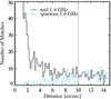 |
Fig. 1 Solid histogram: distance distribution for SDSS quasar counterparts to S1.4 GHz ≥ 1.0 mJy FIRST radio sources. Cyan dashed histogram: distribution for spurious associations, which are obtained by vertically shifting the quasar positions by 1′. |
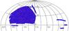 |
Fig. 2 Aitoff projection for the sky coverage of the SDSS DR7 uniform quasar sample from Shen et al. (2011). RQQs are denoted by blue points, while the RLQs are represented by red points. See Sect. 2 for a description of the methodology employed in the selection for the RLQs. |
The sensibility for the FIRST survey is not uniform across the sky, with fluctuations due to different reasons, such as hardware updates, observing strategies, target declination, and increasing noise in the neighborhood of bright sources (Becker et al. 1995). Despite all these potential limitations, the detection limit for most of the targeted sky is a peak flux density of 1 mJy(5σ), with only an equatorial strip having a slightly deeper detection threshold due to the combination of two observing epochs. We refer the interested reader to Helfand et al. (2015), where the impact of all the above mentioned aspects is discussed extensively. The flux limit of 1 mJy is considered only for peak flux density instead of integrated flux density. Hence a source with peak fluxes individually smaller than the detection threshold but with total flux greater than this value could not appear in our radio sample. In particular, lobe-dominated quasars (see Fanaroff & Riley 1974; hereafter FR2) with peak fluxes less than the flux limit suffer from a systematic incompleteness in comparison to core-dominated quasars (FRI). We investigate how not taking into account FIRST resolution effects could possibly affect our RLQ clustering measurements. We estimate the weights for RLQs with fluxes less than 5 mJy using the completeness curve from Jiang et al. (2007b), which takes into account the source morphology and rms values in the FIRST survey for SDSS quasars. We find that including a weighting scheme does not affect the clustering signal for RLQs.
We define a quasar to be radio-loud if it has a detection in the FIRST with a flux above 1 mJy, and radio-quiet if it is undetected in the radio survey. To minimize incompleteness due to the FIRST flux limit while retaining the maximum numbers of quasars for clustering measurements, we consider two radio-luminosity cuts: L1.4 GHz > 4 × 1024 W Hz-1 for 0.3 < z < 1.0; and L1.4 GHz > 1 × 1025 W Hz-1 for 1.0 <z < 2.3. Our parent sample then comprises a total of 45 441 RQQs and 3493 RLQs with 0.3 < z < 2.3, which corresponds to a radio-loud/-quiet source fraction of ~ 7.2%. This ratio is in agreement with previous studied quasar samples (e.g., Jiang et al. 2007a; Hodge et al. 2011). This choice for the redshift range avoids the poor completeness at high-z due to color confusion with stars in the ugri color cube. The sky coverage of our final quasar sample of 6248deg2 is shown in Fig. 2. We calculate the radio-luminosity adopting a mean radio spectral index of αrad = 0.7 (where Sν ∝ ν− α) and applying the usual k-correction for the luminosity estimation. Figure 3 shows the radio-luminosity for our quasar sample. The quasar distribution in the optical-luminosity redshift plane is displayed in Fig. 4. The normalized redshift and optical-luminosity distributions for both samples show a good degree of similarity, this allows a direct comparison of their clustering measurements. We confirm this by applying two Kolmogorov-Smirnov (K-S) tests, which indicate a probability for the redshift and luminosity redshift distributions of 95% and 97%, respectively, that both samples (RLQs and RQQs) are drawn from the same parent distribution.
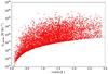 |
Fig. 3 1.4 GHz restframe radio luminosity for the RLQs (red) detected in the FIRST radio survey. We assume a radio spectral index of 0.70, and a flux limit of 1.0 mJy. The dashed lines show the luminosity limit for the FIRST survey flux limit. |
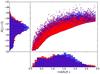 |
Fig. 4 Distribution of RLQs (red) and RQQs (blue) in the optical-luminosity space. The absolute magnitude in the i-band at z = 2Mi(z = 2) is calculated using the K-correction from Richards et al. (2006). The left and bottom panels show the Mi(z = 2) and redshift histograms. The normalized redshift and optical-luminosity distributions are displayed in the left and bottom panels. The normalized distributions for both samples show a good degree of similarity, allowing a direct comparison of their clustering measurements. |
2.4. Final quasar sample
The final spectroscopic quasar sample restricted to 0.3 < z < 2.3 provides an excellent dataset for probing the clustering dependence based on physical properties such as radio-loudness or BH virial mass. It is possible to explore how clustering depends on these properties to some degree across different redshift intervals. Previous quasar clustering studies (e.g., Croom et al. 2005; Ross et al. 2009; Shen et al. 2009) were limited by their sample size (≲ 30 000 quasars) and studied the correlation function for RLQs in only one redshift bin corresponding to the entire redshift range of the sample. We take advantage of the higher quasar numbers of our sample and divide each redshift bin into smaller bins using radio-loudness and the virial BH masses as indicators, and still obtain a good S/N for the correlation function of the samples in our analysis. The MBH−z space is not uniformly populated. We limit our analysis to two mass samples that are separated according to their BH mass:  and
and 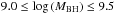 . The redshift distributions for these two mass bins are very different, with more massive BHs peaking at z ~ 2, while less massive at z ~ 0.5 (see Fig. 5). This hampers a direct comparison between their clustering measurements. Thus, we create control samples by randomly selecting quasars from the initial BH mass samples that are matched by their optical luminosity distribution. We verify that the resulting samples can be compared by applying a K-S test to the new redshift distributions. This indicates a probability of 97% that the mass samples are drawn from the same parent distribution. The properties for all the quasar samples are presented in Table 2.
Main properties of our quasar samples.
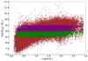 |
Fig. 5 Quasar distribution in the virial BH mass plane. The quasars selected to match in optical luminosity with masses |
3. Clustering of quasars
3.1. Two-point correlation functions
The two-point correlation function (TPCF)  describes the excess probability of finding a quasar at a redshift distance r from a quasar selected randomly over a random distribution. To contraint this function, we create random catalogs with the same angular geometry and the same redshift distribution as the data with at least 70 times the number of quasars in the data sets to minimize the impact of Poisson noise. The redshift distributions corresponding to the different quasar samples are shown by the solid lines in Fig. 6.
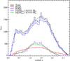 |
Fig. 6 Redshift distributions for the total quasar sample (black), RQQs (blue), RLQs (red), quasars with |
The TPCF is estimated using the minimum variance estimator suggested by Landy & Szalay (1993)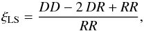 (2)where DD is the number of distinct data pairs, RR is the number of different random pairs, and DR is the number of cross-pairs between the real and random catalogs within the same bin. All pair counts are normalized by nQSO and nR, respectively, the mean number densities in the quasar and random catalogs. We verify our estimates using the Hamilton estimator (Hamilton 1993), and find a good agreement of the results for both estimators within the error bars, although the LS estimator is preferred because it is less sensitive to edge effects.
In reality, observed TPCFs are distorted both at large and small scales. On smaller scales, quasars have peculiar non-linear velocities that cause an elongation along the line of sight, which is referred as the Finger of God effect (Jackson 1972). At larger scales, the coherent motion of quasars that are infalling onto still-collapsing structures produces a flattening of the clustering pattern to the observer. This distortion is called the Kaiser effect (Kaiser 1987).
Because of the existing bias mentioned earlier in redshift-space, a different approach is used to minimize the distortion effects in the clustering signal (Davis & Peebles 1983). Following Fisher et al. (1994), we use the separation vector, s = s1−s2, and the line of sight vector, l = s1 + s2; where s1 and s2 are the redshift-space position vectors. From these, it is possible to define the parallel and perpendicular distances for the pairs as:  (3)Now, we can compute the correlation function
  in a two-dimensional grid using the LS estimator, as in Eq. (2). Because the redshift distortions only affect the distances in the π−direction, we integrate along this component and project it on the rp−axis to obtain the projected correlation function
  (4)which is independent of redshift-space distortions, as it measures the clustering signal as a function of the quasar separation in the perpendicular direction to the line of sight.
In practice, it is not feasible to integrate Eq. (4)to infinity, thus an upper limit πmax to the integral shall be chosen to be a good compromise between the impact of noise and a reliable calculation of the measured signal. We try several π upper limits by fitting wp to a power-law of the form (Davis & Peebles 1983)![Mathematical equation: \begin{equation} w_{p}\left(r_{p}\right)=r_{p}\left(\frac{r_{0}}{r_{p}}\right)^{\gamma}\left[\frac{\Gamma\left(\frac{1}{2}\right)\Gamma\left(\frac{\gamma-1}{2}\right)}{\Gamma\left(\frac{\gamma}{2}\right)}\right], \label{eq:power-law} \end{equation}](/articles/aa/full_html/2017/04/aa26433-15/aa26433-15-eq157.png) (5)where r0 is the real-space correlation length, and γ the power-law slope. We use the range 2.0 ≤ rp ≤ 130 h-1 Mpc to determine the scale at which the clustering signal is stable (Fig. 7). We find that above π = 63.1 h-1 Mpc-1, the fluctuations in the correlation length are within uncertainties and have poorer S/N. Thus, we take this value as our upper integration limit πmax, which is within the range 40−70 h-1 Mpc-1 of previous quasar clustering studies (e.g. Porciani et al. 2004; Ross et al. 2009).
(5)where r0 is the real-space correlation length, and γ the power-law slope. We use the range 2.0 ≤ rp ≤ 130 h-1 Mpc to determine the scale at which the clustering signal is stable (Fig. 7). We find that above π = 63.1 h-1 Mpc-1, the fluctuations in the correlation length are within uncertainties and have poorer S/N. Thus, we take this value as our upper integration limit πmax, which is within the range 40−70 h-1 Mpc-1 of previous quasar clustering studies (e.g. Porciani et al. 2004; Ross et al. 2009).
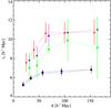 |
Fig. 7 Real-space correlation length r0 vs. the parallel direction to the line of sight π for the full quasar sample (black circles), |
Best-fitting correlation function model parameters for the quasar samples.
3.2. Error estimation
We calculate the errors from the data itself by using the delete-one jackknife method (Norberg et al. 2009). We divide the survey into Nsub different sub-samples, and delete one sample at a time to compute the correlation function for Nsub−1 sub-samples. This process is repeated Nsub times to obtain the correlation function for bin i in the jackknife sub-sample k, denoted by  . We can write the jackknife covariance matrix (e.g. Scranton et al. 2002; Norberg et al. 2009) as
  (6)with ξi the correlation function for all data at each bin i. We employ a total of Nsub = 24 sub-samples for our error estimations. Each sub-sample is chosen to be an independent cosmological volume with approximately the same number of quasars. The off-diagonal elements in the covariance matrix are small at large scales and could potentially insert some noise into the inverse matrix (Ross et al. 2009; Shen et al. 2009). Therefore, we employ only diagonal elements for the χ2 fitting.
3.3. Bias, dark matter halo and black hole mass estimations
According to the linear theory of structure formation, the bias parameter b relates the clustering amplitude of large-scale structure tracers and the underlying dark matter distribution. The quasar bias parameter can be defined as  (7)where wQSO and wDM are the quasar and dark matter correlation functions (Peebles 1980), respectively. We estimate the bias factor using the halo model approach, in which wDM has two contributions: the 1-halo and 2-halo terms. The first term is related to quasar pairs from within the same halo, and the second one is the contribution from quasars pairs in different haloes. As the latter term dominates at large separations, we can neglect the 1-halo term and write wDM as (Hamana et al. 2002)
 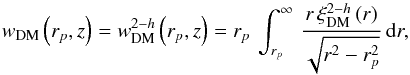 (8)with
  (9)where k is the wavelength number, h refers to the halo term,
  is the Fourier transform of the linear power spectrum (Efstathiou et al. 1992) and
  is the spherical Bessel function of the first kind.
With the bias factor, it is possible to derive the typical mass for the halo in which the quasars reside. We follow the procedure described in previous AGN clustering studies (e.g., Myers et al. 2007; Krumpe et al. 2010; Allevato et al. 2014b) using the ellipsoidal gravitational collapse model of Sheth et al. (2001) and the analytical approximations of van den Bosch (2002).
4. Results
4.1. Projected correlation function wp (rp)
First, we check the consistency of our results by calculating the real-space TPCF for the entire quasar sample in the interval 0.3 ≤ z ≤ 2.3 and compare it with previous clustering studies. We select a fitting range of 2 ≤ rp ≤ 130 h-1 Mpc to have a distance coverage similar to previous quasar clustering studies (e.g., Shen et al. 2009). To determine the appropriate values for our TPCFs, we fit Eq. (5)with r0 and γ as free parameters using a χ2 minimization technique. We find a real-space correlation length of  and a slope of
  , which is in good agreement with the results of Ross et al. (2009) for the SDSS DR5 quasar catalog, and Ivashchenko et al. (2010) for their SDSS DR7 uniform quasar catalog. Subsequently, we derive the best-fit r0 and γ values for all the quasars samples. The best-fitting values and their respective errors are presented in Table 2.
We then split each redshift range according to their radio-loudness and virial BH mass to study the clustering dependence on these properties. The results of our clustering analysis for the different quasar sub-samples as a function of radio-loudness are presented in the left panels of Fig. 9.
The best-fitting parameters in the interval 0.3 ≤ z ≤ 2.3 are  ,
,  for the RLQs and
 for the RQQs (see Table 2). The latter fit is poor with χ2 = 19.60 and 7 d.o.f., while the former, with the same number of data points, is more acceptable, with χ2 = 1.06. It is clear from our clustering measurements that RLQs are more strongly clustered than RQQs. The two additional redshift bins show similar trends, with RLQs in the low-z bin clustering more strongly.
In order to check our results, we estimate the correlation function for 100 randomly selected quasar sub-samples chosen from the RQQs with the same number of quasars as RLQs in the corresponding redshift interval. The randomly selected quasar samples present similar clustering lengths to those of RQQs.
We also fit the correlation function over a more restricted range to examine the impact of different distance scales on the clustering measurements. Using 2 ≤ rp ≤ 35 h-1 Mpc, we obtain a model with a somewhat smaller correlation scale-length  and a flatter slope
  for RQQs in the full sample. The model matches the data better, resulting in χ2 = 1.06 and 4 d.o.f. This may signal a change in the TPCF with scale; the transition between the one-halo and two-halo terms may be responsible for the
  distortion on smaller scales (e.g., Porciani et al. 2004). Our remaining non-radio samples show a similar trend of improving the fits at smaller distances. For RLQs, we obtain
  with χ2 = 2.77 and 4 d.o.f. The changes in the parameters are within the error bars.
We use the virial BH mass estimations based on single-epoch spectra to investigate whether or not quasar clustering depends on BH mass. The emission line which is employed to determine the fiducial virial mass depends on the redshift interval (see Shen et al. 2008 for a description).
First, we divide the quasar samples using the median virial BH mass in redshift intervals of △ z = 0.05 following Shen et al. (2009). Although this approach yields samples with comparable redshift distributions, it mixes quasars regardless of their luminosity and could wash out any true dependence on MBH. Indeed, the mass samples following this scheme hardly show any significant differences in their clustering with correlation lengths similar to those of RQQs. Thus, we proceed to create mass samples with two MBH intervals: and , as described in Sect. 2.4. The right-hand panels in Fig. 9 show wp(rp) for these BH mass-selected samples. It can be seen that quasars with higher BH masses have stronger clustering. For 0.3 ≤ z ≤ 2.3, we obtain  ,
,  for quasars with ; and
  ,
,  for BH masses in the range . In the other z-bins, the resulting trend is similar, with the low-z bin showing the larger clustering amplitudes. These trends hold when the distance is restricted to 2 ≤ rp ≤ 35 h-1 Mpc, with no significant variations in r0 and γ due to the larger uncertainties at these scales.
4.2. Quasar bias factors
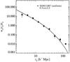 |
Fig. 8 Real-space correlation function for the SDSS DR7 quasar uniform sample with 0.3 ≤ z ≤ 2.3. The solid line denotes the model |

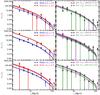 |
Fig. 9 Projected correlation functions for the radio-loudness (left) and BH mass (right) samples corresponding to the redshift intervals defined in Table 2. The thin lines in each panel represent the term |

We compute the quasar bias factors over the scales 2.0 ≤ rp ≤ 130 h-1 Mpc using the  model in Eq. (8). Again, this distance scale has been chosen to have a good overlap with previous SDSS quasar clustering studies (e.g., Shen et al. 2009; Ross et al. 2009). The best-fit bias values and the corresponding typical DMH masses for quasar samples are shown in Table 2. We find that the SDSS DR7 quasars at
  (Fig. 8) have a bias of b = 2.00 ± 0.08. Previous bias estimates from 2QZ (Croom et al. 2005) and 2SLAQ (da Ângela et al. 2008) surveys are consistent with our results within the 1σ error bars.
The left panel in Fig. 9 compares the projected real-space TPCF wp/rp for the RLQs (red) and RQQs (blue). Optically selected quasars are significantly less clustered than radio quasars in the three redshift bins analyzed, which implies that they are less biased objects. Indeed, the RLQs and RQQs, with mean redshifts of  and
and  , have bias equivalent to b = 3.14 ± 0.34 and b = 2.01 ± 0.08, respectively. These bias factors correspond to typical DMH masses of
 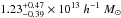 and
and  , respectively. We obtain similar results for RQQs in the other two redshift bins with
  and
and  , respectively, (see Table 2). There are considerable differences between the low-z and high-z bins results for RLQs, with low-z RLQs residing in more massive haloes with masses of
 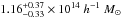 .
.
The projected correlation functions for the mass samples are shown in Fig. 9 (right panels), and the corresponding best-fit bias parameters are reported in Table 2. We find b = 2.64 ± 0.42 for quasars with , and b = 2.99 ± 0.43 for the objects with in the full redshift interval. There is a clear trend: the quasars powered by the most massive BHs are more clustered than quasars with less massive BHs. These quasars are more biased than RQQs, but less than radio quasars. In the other z-bins, the b values are comparable to those of the full sample. This implies larger halo masses for the low-z quasars.
We also estimate the bias over 2.0 ≤ rp ≤ 35 h-1 Mpc. RQQs in the three bins show hardly almost no difference within the uncertainties. The resulting bias for RLQs is b = 3.11 ± 0.42 at 0.3 ≤ z ≤ 2.2, which is approximately 1% smaller in comparison to the bias at 2.0 ≤ rp ≤ 130 h-1 Mpc. Therefore, restricting the bias does not affect our conclusions for the radio samples. For the mass samples, they remain virtually the same when the range is restricted.
4.3. Bias and host halo mass redshift evolution
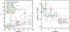 |
Fig. 10 Left: derived linear bias parameter b as a function of redshift for radio and optical AGN samples represented by the corresponding legend. Red or gray triangles represent the RLQs or RQQs sub-samples of this work, respectively. The dashed lines denote the expected redshift evolution of DMH masses based on the models from Sheth et al. (2001) with |
![Mathematical equation: \hbox{$\log\,\left(M_{\textrm{DM}}/h^{-1}~M_{\odot}\right)=\left[12.0,\,13.0,\,13.5,\,14.0\right]$}](/articles/aa/full_html/2017/04/aa26433-15/aa26433-15-eq312.png)
![Mathematical equation: \hbox{$\log\,\left(M_{\textrm{DM}}/h^{-1}~M_{\odot}\right)=\left[12.4,\,13.41\right].$}](/articles/aa/full_html/2017/04/aa26433-15/aa26433-15-eq314.png)
In Fig. 10 (left panel), we show our bias estimates for RQQs and RLQs (red and gray triangles, respectively). It can be seen that the bias is a strong function of redshift. In the same plot, we show the previous bias estimates from the optical spectroscopic quasar samples (gray symbols) as well as radio-loud AGNs (green and orange symbols). Our estimates for both RQQs and RLQs are consistent with previous works. The expected redshift evolution tracks of DMH masses based on the models from Sheth et al. (2001) are shown by dashed lines in Fig. 10. RQQs follow a track of constant mass a few times 1012h-1M⊙, while the majority of RLQs and radio sources approximately follow a track of ~ 1014.0−13.5h-1M⊙ within the error bars.
4.4. Clustering as a function of radio-loudness
Even though the number of radio sources is only ~ 7.6% of the total number of quasars, it is clear from the left-hand panels of Fig. 9 that RLQs are considerably more clustered than RQQs in all the redshift bins. The stronger clustering presented by RLQs suggests that these inhabit more massive haloes than their radio-quiet counterparts. The RLQs typical halo mass of > 1 × 10¹³h-1M⊙ is characteristic of galaxy groups and small clusters, while the typical mass of a few times 1012h-1M⊙ for RQQs is typical of galactic haloes. The higher DMH mass presented by RLQs in the low-z bin is similar to the halo mass of galaxy clusters, which is usually > 1 × 10¹⁴h-1M⊙.
The right-hand panel in Fig. 10 presents the DMH masses against redshift for the same samples as in the left-hand panel. Our new mass estimates for RLQs and RQQs are generally consistent with those derived in previous works (e.g., Croom et al. 2005; Porciani & Norberg 2006; Ross et al. 2009; Shen et al. 2009). We denote the typical halo masses for the two quasar populations using dashed lines. This suggests that the difference between the typical host halo masses for RLQs and RQQs is constant with redshift, with the haloes hosting RLQs being approximately one order of magnitude more massive.
4.5. Clustering as function of BH masses
Our clustering measurements for the and show a clear dependence on virial BH masses. This trend is apparent in Fig. 9 (right panels) for all the redshift bins considered. Moreover, this is reflected in our MBH predictions for the mass samples in Fig. 11. The quasars powered by SMBHs with present larger clustering amplitudes than those with less massive BH masses in the range . Table 2 indicates that both RLQs and the quasars with BH masses of have larger correlation lengths than RQQs and quasars with . However, RLQ clustering is at least slightly stronger in all the redshift bins analyzed. It is important to remark that the use of virial estimators to calculate the BH masses is subject to large uncertainties (e.g., Shen et al. 2008; Shen & Liu 2012; Assef et al. 2012) leading to significant biases and scatter around the true BH mass values, which could potentially weaken any clustering dependence on BH mass. Nevertheless, our results and recent studies (Komiya et al. 2013; Krumpe et al. 2015) give some validity to their use in clustering analyses.
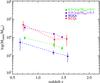 |
Fig. 11 Ratio between the DMH and the average virial BH masses for our quasar samples as a function of redshift. |
Figure 11 shows the redshift evolution of the ratio between the DMH and the average virial BH masses for our quasar samples. The different lines mark the ratio for each quasar sample denoted by the plot legend. The ratios reproduce the trend for the clustering amplitudes in all the samples: RLQs and quasars with cluster more strongly than RQQs and quasars with , respectively. Quasars with present clustering comparable to RLQs. Also, it is evident that the ratios are larger at low-z due to the host haloes being more massive and the virial BH masses showing no significant changes with redshift (see Table 1).
An important point to consider is the cause of stronger clustering: is the stronger clustering for the high-mass quasars due to the fact that they are radio loud, or are the RLQs more clustered due to the fact that they have higher BH masses. We can address this by examining the distribution of RLQs on the virial BH mass plane. This distribution is not restricted to high BH masses only. Instead, RLQs present BH masses in all the ranges sampled, indicating that their radio-emission rather than high BH mass is responsible for the stronger clustering in RLQs. However, for the high-mass sample only a fraction of ~ 6% is radio-loud, which translates to approximately 700 RLQs, which is not large enough to obtain a reliable clustering signal. For the high-mass sample minus the radio-quasars, we do obtain a clustering amplitude similar to those including radio objects. Therefore, we conclude that the stronger clustering for both samples is mainly due to the intrinsic properties of each sample. This point needs to be addressed using forthcoming quasar samples with higher quasar numbers.
4.6. Clustering as a function of redshift
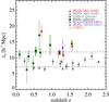 |
Fig. 12 Different values for the real-space correlation length r0 against redshift for RLQs and RQQs from SDSS DR5 (purple and gray downward triangles, Shen et al. 2009), optical quasars (gray circles, Croom et al. 2005; Ross et al. 2009; Eftekharzadeh et al. 2015), radio galaxies (dark green squares, Peacock & Nicholson 1991; Magliocchetti et al. 2004; Wake et al. 2008; Fine et al. 2011; Lindsay et al. 2014b), and FSRQs (orange star, Allevato et al. 2014a). The r0 values for RLQ and RRQ in our sample are represented by red and gray upward triangles, respectively. For comparison, we show the r0 values corresponding to r0 = [11.8, 7.1] h-1 Mpc (dashed lines). The results from Lindsay et al. (2014b) are derived assuming linear clustering. |
In Fig. 12, we show our r0 measurements along with results from previous works for radio galaxies (Peacock & Nicholson 1991; Magliocchetti et al. 2004; Wake et al. 2008; Fine et al. 2011; Lindsay et al. 2014b; Allison et al. 2015; Nusser & Tiwari 2015), optically-selected quasars (Ross et al. 2009; Croom et al. 2005; Eftekharzadeh et al. 2015), and γ−selected blazars (Allevato et al. 2014a). In these samples, the typical 1.4 GHz radio-luminosities for AGNs is 1023−1026 W Hz-1 which is representative of FRI sources, whilst for our sample the average radio-luminosity is ~ 8 × 1026 W Hz-1, which is near the boundary between FRI and FRII sources.
A systematic trend with redshift is observed in Fig. 12, which indicates that the majority of radio sources considered have clustering lengths over the entire redshift range considered (0 <z< 2.3). This is consistent with the trend from Fig. 10, where the majority of radio sources seem to inhabit haloes of MDMH> 1 × 10¹³ at all redshifts. The simplest interpretation of this result is that a considerable part of the bright radio population resides in massive haloes with large correlation lengths. Our new RLQ clustering measurements for the full sample and high-z bin agree, within the errors bars, with the previous single estimation from Shen et al. (2009) using the SDSS DR5 quasar sample, while the low-z bin correlation amplitude is consistent with Lindsay et al. (2014b).
Overzier et al. (2003) measured the angular TPCF for the NVSS survey (Condon et al. 1998) and concluded that lower luminosity radio sources (≤ 1026 W Hz-1) present typical correlation lengths of r0 ≲ 6 h-1 Mpc, whilst the brighter radio sources (> 1026 W Hz-1), mainly FRII type, have significantly larger scale lengths of r0 ≳ 14 h-1 Mpc. Our findings are consistent with Overzier et al. (2003) predictions for the bright radio population. It is possible that the weaker correlation length presented by lower radio-luminosity samples in Fig. 12 indicates a mild clustering dependence on radio-luminosity. However, our RLQs sample is still too small to draw firm conclusions on the radio luminosity dependence as the increasing errors for these luminosity-limited samples mean we cannot satisfactorily distinguish between them
The DMH masses for RLQs and quasars with at 0.3 <z< 1.0, are approximately > 1 × 10¹⁴h-1M⊙, which is the typical value for cluster-size haloes. Moreover, these halo masses are larger than the corresponding haloes for quasar samples at z> 1.0. This suggests that the environments in which these objects reside is different from those of their high-z counterparts. Additionally, the radio source clustering amplitudes are similar to the clustering scale of massive galaxy clusters (e.g., Bahcall et al. 2003). This almost certainly reveals a connection between quasar radio-emission and galaxy cluster formation that must be explored in detail with data from forthcoming radio surveys.
4.7. Clustering and AGN unification theories
Our clustering results hint at an interesting point regarding the relationship between RLQs and radio galaxies in AGN classifications, which consider these AGNs as the same source type seen from different angles (e.g., Urry & Padovani 1995). Thus, we would expect that different AGN types such as radio galaxies and RLQs, should have similar clustering properties. The real-space correlation lengths for RLQs (red triangles) and other radio sources including, radio galaxies (green squares), are shown in Fig. 12. We see that there is a reasonable consistency for most r0 values up to z ≲ 2.3. We identify the same trend in Fig. 10 (right panel), where bright radio sources seem to inhabit haloes of approximately constant mass of ≳ 1013.5h-1M⊙. Our clustering study seems to support the validity of unification models at least for RLQs and radio galaxies with relatively median radio-luminosities (≳ 1 × 10²³ W Hz-1).
Allevato et al. (2014a) studied the clustering properties of a γ−selected sample of blazars divided into BL Lacs and flat-spectrum radio quasars (FSRQs). In the context of unification models, FSRQs are associated with intrinsically powerful FRII radio galaxies, while BL Lacs are related to weak FRI radio galaxies. From a clustering point of view, as explained before, luminous blazars should have similar clustering properties to radio galaxies. In Figs. 10 and 12, we denote by a orange star, the DMH mass and correlation length for FSRQs, respectively, found by Allevato et al. (2014b). FSRQs show a similar MDMH value to those of radio galaxies and RLQs, supporting a scenario in which radio AGNs such as quasars, radio galaxies and powerful blazars are similar from a clustering perspective and reside in massive hosting haloes providing the ideal place to fuel the most massive and powerful BHs.
Based on an analysis of the cross-correlation function for radio galaxies, RLQs and a reference sample of luminous red galaxies Donoso et al. (2010) concluded that the clustering for RLQs is weaker in comparison with radio galaxies. This is apparently at odds with previous clustering measurements and our results. However, there are several differences between Donoso’s and our sample that must be considered. First, Donoso’s sample is significantly smaller with only 307 RLQs at 0.35 <z< 0.78. Secondly, in the common range between the two samples where the TPCF is computed, their clustering signal has large uncertainties. Thirdly, they compute the clustering for objects with radio-luminosities restricted to > 1025 W Hz-1. We employ the same luminosity cut only for the high-z bin, while for the low-z bin only sources brighter than > 4 × 1024 W Hz-1 are considered. The mean luminosity for both redshift bins is > 2 × 1026 W Hz-1 (see Table 1). Therefore, comparable radio-luminosity cuts were used for both samples. For these reasons, it is difficult to draw any conclusions from comparison with the Donoso results.
4.8. The role of mergers in quasar radio-activity
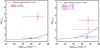 |
Fig. 13 Bias parameter b as a function of bolometric luminosity for our RLQs and RQQs in the ranges 0.3 ≤ z ≤ 1.0 (left) and 1.0 ≤ z ≤ 2.0 (right). Errors in the Lbol axis are the dispersion values for each different quasar sample. The solid lines in both panels denote the predicted bias luminosity evolution according to the Shen (2009) model, which predicts that quasar activity is triggered by galaxy mergers. |
We compare our clustering measurements with the theoretical framework for the growth and evolution of SMBHs introduced by Shen (2009). This model links the quasar properties and host halo mass with quasar activity being triggered by major galaxy mergers. The bias factor is a function of the instantaneous luminosity and redshift, with most luminous quasars having larger host-halo masses. The rate of quasar activity is controlled by the fraction parameter fQSO, which involves exponential cutoffs at both high and low mass ends assigned according to phenomenological rules. At low masses, the cutoffs prevent quasar activity on the smallest postmerger haloes, while those at the highest masses cause that gas accretion to become inefficient and subsequent BH growth stops. Figure 13 presents the predicted linear bias as a function of bolometric luminosity at z = 0.65 (left) and z = 1.40 (right). In the low-z bin (0.3 ≤ z ≤ 1.0), the model can reproduce the bias for the RQQs. However, the quasar merger model disagrees with the higher bias value for RLQs. At high-z(1.0 ≤ z ≤ 2.3), the consistency between the model predictions and the measured bias for RQQs for the high-z bin and the complete quasar sample worsens. The bias luminosity-dependent trend predicted by the model seems to be followed slightly better by the RLQs than in the low-z bin.
The discrepancy between the merger-driven model predictions and our bias values might indicate differences in the fueling channels for both quasar types. First, our bias estimates for RQQs in the context of the Shen et al. (2009) framework favor accretion of cold gas via galaxy mergers (referred to as cold-gas accretion). These MDH masses are in agreement with the halo mass-scale of a few times ≳ 1012h-1M⊙ predicted by merger-driven models for optical quasars (e.g., Croom et al. 2005; Ross et al. 2009). In contrast, the bias results for RLQs, which correspond to halo masses of ≳ 1013h-1M⊙, cannot be reproduced by models that assume that quasar activity is solely triggered by typical galaxy mergers.
A similar difference in DMH masses has been reported in clustering studies for X-ray selected AGNs with moderate luminosity  (Gilli et al. 2005, 2009; Starikova et al. 2011; Allevato et al. 2011; Mountrichas et al. 2013; Mountrichas & Georgakakis 2012). The DMH masses of X-ray AGNs are approximately 1013h-1M⊙, which is significantly higher in comparison with relatively bright optical quasars
  with ≳ 1012h-1M⊙ (Croom et al. 2005; Ross et al. 2009). Several authors have observationally (Allevato et al. 2011; Mountrichas & Georgakakis 2012; Allevato et al. 2014b) and theoretically (Fanidakis et al. 2012, 2013a) interpreted these two mass scales as evidence favoring different accretion channels for each AGN population. Fanidakis et al. (2013a), using semi-analytical galaxy formation models, found that cold gas fuelling cannot reproduce the DMH masses from X-ray AGN clustering studies. Instead, they found that when gas cooled from quasi-hydrostatic hot-gas haloes (i.e., known as hot-mode; Croton et al. 2006) is included, a much better agreement with the DMH masses derived from X-ray AGN clustering studies is obtained.
The differences in DMH masses for X-ray AGNs and optical quasars is reminiscent of our results for RQQs and RLQs. This may suggest that the contribution of hot-gas accretion increases for more massive haloes, such as those hosting X-ray AGNs and RLQs. However, this scenario for RLQs still needs to be confronted with more detailed simulations and models to further constrain the physics of BH accretion.
4.9. Black hole properties involved in quasar triggering
As considering only cold accretion via mergers cannot explain the mass scales associated with RQQs and RLQs, it is important to take into account different mechanisms related to quasar activity. For instance, the massive haloes where these RLQs are embedded must have an important role in determining the BH properties and the onset of radio activity. Indeed, the BH spin could be altered by environmental conditions: either by means of coherent gas accretion, or by BH-BH mergers. In the spin paradigm proposed by Wilson & Colbert (1995), the rapidly spinning BHs are associated with radio-loud AGNs, whilst the slower spinning ones are considered to be radio-quiet. Objects above a certain spin threshold could have the necessary energy to produce powerful relativistic jets (Blandford & Znajek 1977). The intrinsic scatter on the BH spin values required to power the jets may reproduce the different morphologies and the shape of the luminosity function at radio wavelengths (Fanidakis et al. 2011). Another plausible scenario is a two-way interaction between RLQs jets and the surrounding intergalactic medium, as suggested by the morphological associations of radio continuum with extended optical emission (van Breugel et al. 1985), and bent radio structures in nearby radio active galaxies (O’Dea & Owen 1986). As radio jets propagate into a dense interstellar medium they suffer from both depolarization and decollimation that yield an enhancement in their radio brightness (Begelman et al. 1984). The luminosity boosting for these objects may help to make them just bright enough to be detectable above the FIRST survey flux limit. Finally, the magnetic field configurations derived from polarimetry studies (e.g., Bridle & Perley 1984) indicate that the magnetic field in FR-II radio-galaxies is predominantly aligned along the jet for most of its length, whereas FR-I objects are characterized by perpendicular and parallel components. This may suggest a correlation between the DMH mass and the efficiency in producing the magnetic field alignment required to produce brighter radio emission.
In conclusion, the interplay between all these BH properties in triggering radio activity is still poorly understood. Additional observational and theoretical efforts are required to obtain a better comprehension of the origins of radio-emission in quasars.
5. Summary
In this study, we have investigated the quasar clustering dependence on radio-loudness and BH virial mass, by using a sample of approximately 48 000 spectroscopically confirmed quasars at 0.3 ≤ z ≤ 2.3 drawn from SDSS DR7 quasar catalog (Shen et al. 2011; Schneider et al. 2010). Our radio sample consists of FIRST-detected quasars. The main conclusions of this paper are the following:
-
1.
We studied the spatial clustering of quasars at 0.3 ≤ z ≤ 2.3 over the scales 2.0 ≤ r0 ≤ 130 h-1 Mpc.For RQQs, we find a real-space correlation length equal to
 with aslope of . RLQs are more strongly clustered than RQQs with
  , .
, . -
2.
We estimated the linear bias for RQQs and RLQs by splitting the quasar sample according to radio-loudness, and find b = 2.01 ± 0.08 and b = 3.14 ± 0.34, respectively, for the full redshift interval.
-
3.
We investigated the clustering dependency on BH virial mass using quasar samples with
and constructed to have comparable optical luminosity distributions. We find a dependence on BH mass, with the quasars powered by the most massive BHs having larger correlation lengths. These results suggest that BH virial mass estimations based on broad emission lines may be valid BH mass proxies for clustering studies. -
4.
Using our best-fit bias values, we find that RLQs in our sample inhabit massive haloes with masses of MDMH ≳ 1013.5h-1M⊙ at all redshifts, which corresponds to the mass scale of galaxy groups and galaxy clusters. RQQs reside in less massive haloes of a few times ~ 1012h-1M⊙.
-
5.
RQQs have smaller DMH masses in comparison with RLQs. The BH mass selected samples have larger DMH masses than RQQs, but smaller DMH masses than those of radio quasars. However, RLQs have the most massive DMHs in all the redshift bins considered. We considered the ratio between the DHM and average virial BH masses for all the samples. The ratios present the same above-mentioned trends.
-
6.
Within our quasar sample, we do detect significant correlations between quasar clustering and redshift for RLQs up to z ≲ 2.3. At low-z, RLQs and quasars with
have clustering amplitudes of r0 ≳ 18 h-1 Mpc, comparable to those of today’s massive galaxy clusters. Our real-space clustering length r0 estimate for the full samples agrees very well with the majority of previous complementary and independent clustering estimates for radio galaxies and RLQs. -
7.
We used radio-loudness to separate the quasar sample into RLQs and RQQs. Our clustering measurements suggest that there are differences between RLQs and RQQs in terms of halo and BH mass scales. Our result is consistent with the hierarchical clustering scenario, in which most massive galaxies harboring the most massive BHs form in the highest density peaks, thus cluster more strongly than less massive galaxies in typical peaks. This is confirmed by clustering analysis of the mass samples and their dependence on MBH.
-
8.
Comparing our linear bias and DMH mass estimates with the theoretical predictions of the merger-driven model from Shen (2009), we find that this model cannot explain the larger bias and DHM masses for RLQs, suggesting that cold accretion driven by galaxy mergers is unlikely to be the main fueling channel for RLQs with
 . Conversely, merger model predictions agree well with our bias and host mass estimates for RQQs, with MDMH ≳ 1012h-1M⊙.
 -
9.
The disagreement between the bias luminosity-dependent trend predicted by the Shen (2009) merger model and our bias estimates for RLQs suggests a scenario where the radio emission is a complex phenomenon that may depend on several BH properties such as: BH spin, environment, magnetic field configuration, and accretion physics.
-
10.
The similarity in clustering amplitude and host halo masses for radio-galaxies, radio-selected AGNs, RLQs, and FSRQs is in line with the idea that the different spectral features for these radio sources depend only on the orientation angle and not on the environment in which they are embedded, supporting orientation-driven unification models (Urry & Padovani 1995, and references therein). Donoso et al. (2010) found that the clustering properties for RLQs and radio galaxies differ, with the latter displaying a stronger clustering. In principle, these results are in tension with our results and previous clustering studies of radio sources (e.g. Magliocchetti et al. 2002; Wake et al. 2008; Shen et al. 2009). However, their small sample size and large uncertainties in the clustering in comparison with our sample make it difficult to draw any significant conclusions. In future studies, larger samples of quasars and radio galaxies may provide new information about the clustering properties for both populations.
Acknowledgments
E.R.M. wish to thank F. Mernier and E. Rigby for critical reading and F. Shankar for providing us the tracks in Fig. 13. E.R.M. acknowledges financial support from NWO Top project, No. 614.001.006. H.R. acknowledges support from the ERC Advanced Investigator program NewClusters 321271. Moreover, we would like to thank the referee for valuable suggestions on the manuscript. Funding for the SDSS and SDSS-II has been provided by the Alfred P. Sloan Foundation, the Participating Institutions, the National Science Foundation, the US Department of Energy, the National Aeronautics and Space Administration, the Japanese Monbukagakusho, the Max Planck Society, and the Higher Education Funding Council for England. The SDSS Web Site is http://www.sdss.org/. The SDSS is managed by the Astrophysical Research Consortium for the Participating Institutions. The Participating Institutions are the American Museum of Natural History, Astrophysical Institute Potsdam, University of Basel, University of Cambridge, Case Western Reserve University, University of Chicago, Drexel University, Fermilab, the Institute for Advanced Study, the Japan Participation Group, Johns Hopkins University, the Joint Institute for Nuclear Astrophysics, the Kavli Institute for Particle Astrophysics and Cosmology, the Korean Scientist Group, the Chinese Academy of Sciences (LAMOST), Los Alamos National Laboratory, the Max-Planck-Institute for Astronomy (MPIA), the Max-Planck-Institute for Astrophysics (MPA), New Mexico State University, Ohio State University, University of Pittsburgh, University of Portsmouth, Princeton University, the United States Naval Observatory, and the University of Washington.
References
- Adelberger, K. L., Steidel, C. C., Pettini, M., et al. 2005, ApJ, 619, 697 [NASA ADS] [CrossRef] [Google Scholar]
- Allevato, V., Finoguenov, A., Cappelluti, N., et al. 2011, ApJ, 736, 99 [NASA ADS] [CrossRef] [Google Scholar]
- Allevato, V., Finoguenov, A., & Cappelluti, N. 2014a, ApJ, 797, 96 [NASA ADS] [CrossRef] [Google Scholar]
- Allevato, V., Finoguenov, A., Civano, F., et al. 2014b, ApJ, 796, 4 [NASA ADS] [CrossRef] [Google Scholar]
- Allison, R., Lindsay, S. N., Sherwin, B. D., et al. 2015, MNRAS, 451, 849 [NASA ADS] [CrossRef] [Google Scholar]
- Antonucci, R. 1993, ARA&A, 31, 473 [Google Scholar]
- Assef, R. J., Frank, S., Grier, C. J., et al. 2012, ApJ, 753, L2 [NASA ADS] [CrossRef] [Google Scholar]
- Bahcall, N. A., Dong, F., Hao, L., et al. 2003, ApJ, 599, 814 [NASA ADS] [CrossRef] [Google Scholar]
- Barone-Nugent, R. L., Trenti, M., Wyithe, J. S. B., et al. 2014, ApJ, 793, 17 [NASA ADS] [CrossRef] [Google Scholar]
- Becker, R. H., White, R. L., & Helfand, D. J. 1995, ApJ, 450, 559 [NASA ADS] [CrossRef] [Google Scholar]
- Begelman, M. C., Blandford, R. D., & Rees, M. J. 1984, Rev. Mod. Phys., 56, 255 [NASA ADS] [CrossRef] [Google Scholar]
- Best, P. N., Kauffmann, G., Heckman, T. M., et al. 2005, MNRAS, 362, 25 [NASA ADS] [CrossRef] [Google Scholar]
- Blandford, R. D., & Znajek, R. L. 1977, MNRAS, 179, 433 [NASA ADS] [CrossRef] [Google Scholar]
- Blanton, M. R., Lin, H., Lupton, R. H., et al. 2003, AJ, 125, 2276 [NASA ADS] [CrossRef] [Google Scholar]
- Bonoli, S., Marulli, F., Springel, V., et al. 2009, MNRAS, 396, 423 [NASA ADS] [CrossRef] [Google Scholar]
- Bridle, A. H., & Perley, R. A. 1984, ARA&A, 22, 319 [NASA ADS] [CrossRef] [Google Scholar]
- Bridle, A. H., Hough, D. H., Lonsdale, C. J., Burns, J. O., & Laing, R. A. 1994, AJ, 108, 766 [NASA ADS] [CrossRef] [Google Scholar]
- Brown, M. J. I., Webster, R. L., & Boyle, B. J. 2000, MNRAS, 317, 782 [NASA ADS] [CrossRef] [Google Scholar]
- Chiaberge, M., & Marconi, A. 2011, MNRAS, 416, 917 [NASA ADS] [CrossRef] [Google Scholar]
- Cirasuolo, M., Magliocchetti, M., Celotti, A., & Danese, L. 2003, MNRAS, 341, 993 [NASA ADS] [CrossRef] [Google Scholar]
- Coil, A. L., Newman, J. A., Cooper, M. C., et al. 2006, ApJ, 644, 671 [NASA ADS] [CrossRef] [Google Scholar]
- Colless, M., Dalton, G., Maddox, S., et al. 2001, MNRAS, 328, 1039 [NASA ADS] [CrossRef] [Google Scholar]
- Condon, J. J., Cotton, W. D., Greisen, E. W., et al. 1998, AJ, 115, 1693 [NASA ADS] [CrossRef] [Google Scholar]
- Croom, S. M. 2011, ApJ, 736, 161 [NASA ADS] [CrossRef] [Google Scholar]
- Croom, S. M., Smith, R. J., Boyle, B. J., et al. 2004, MNRAS, 349, 1397 [NASA ADS] [CrossRef] [Google Scholar]
- Croom, S. M., Boyle, B. J., Shanks, T., et al. 2005, MNRAS, 356, 415 [NASA ADS] [CrossRef] [Google Scholar]
- Croton, D. J., Springel, V., White, S. D. M., et al. 2006, MNRAS, 365, 11 [NASA ADS] [CrossRef] [Google Scholar]
- da Ângela, J., Shanks, T., Croom, S. M., et al. 2008, MNRAS, 383, 565 [NASA ADS] [CrossRef] [Google Scholar]
- Daddi, E., Röttgering, H. J. A., Labbé, I., et al. 2003, ApJ, 588, 50 [NASA ADS] [CrossRef] [Google Scholar]
- Davies, R. I., Thomas, J., Genzel, R., et al. 2006, ApJ, 646, 754 [NASA ADS] [CrossRef] [Google Scholar]
- Davis, M., & Peebles, P. J. E. 1983, ApJ, 267, 465 [NASA ADS] [CrossRef] [Google Scholar]
- de Francesco, G., Capetti, A., & Marconi, A. 2006, A&A, 460, 439 [NASA ADS] [CrossRef] [EDP Sciences] [Google Scholar]
- de Francesco, G., Capetti, A., & Marconi, A. 2008, A&A, 479, 355 [NASA ADS] [CrossRef] [EDP Sciences] [Google Scholar]
- Di Matteo, T., Springel, V., & Hernquist, L. 2005, Nature, 433, 604 [NASA ADS] [CrossRef] [PubMed] [Google Scholar]
- DiPompeo, M. A., Hickox, R. C., & Myers, A. D. 2016, MNRAS, 456, 924 [NASA ADS] [CrossRef] [Google Scholar]
- Donoso, E., Li, C., Kauffmann, G., Best, P. N., & Heckman, T. M. 2010, MNRAS, 407, 1078 [NASA ADS] [CrossRef] [Google Scholar]
- Doroshenko, V. T., Sergeev, S. G., Klimanov, S. A., Pronik, V. I., & Efimov, Y. S. 2012, MNRAS, 426, 416 [NASA ADS] [CrossRef] [Google Scholar]
- Dunlop, J. S., McLure, R. J., Kukula, M. J., et al. 2003, MNRAS, 340, 1095 [NASA ADS] [CrossRef] [Google Scholar]
- Efstathiou, G., Bond, J. R., & White, S. D. M. 1992, MNRAS, 258, 1 [NASA ADS] [CrossRef] [Google Scholar]
- Eftekharzadeh, S., Myers, A. D., White, M., et al. 2015, MNRAS, 453, 2779 [NASA ADS] [CrossRef] [Google Scholar]
- El Bouchefry, K., & Cress, C. M. 2007, Astron. Nachr., 328, 577 [NASA ADS] [CrossRef] [Google Scholar]
- Fan, X., Narayanan, V. K., Lupton, R. H., et al. 2001, AJ, 122, 2833 [NASA ADS] [CrossRef] [Google Scholar]
- Fanaroff, B. L., & Riley, J. M. 1974, MNRAS, 167, 31P [Google Scholar]
- Fanidakis, N., Baugh, C. M., Benson, A. J., et al. 2011, MNRAS, 410, 53 [NASA ADS] [CrossRef] [Google Scholar]
- Fanidakis, N., Baugh, C. M., Benson, A. J., et al. 2012, MNRAS, 419, 2797 [NASA ADS] [CrossRef] [Google Scholar]
- Fanidakis, N., Georgakakis, A., Mountrichas, G., et al. 2013a, MNRAS, 435, 679 [NASA ADS] [CrossRef] [Google Scholar]
- Fanidakis, N., Macciò, A. V., Baugh, C. M., Lacey, C. G., & Frenk, C. S. 2013b, MNRAS, 436, 315 [NASA ADS] [CrossRef] [Google Scholar]
- Fernandes, C. A. C., Jarvis, M. J., Rawlings, S., et al. 2011, MNRAS, 411, 1909 [NASA ADS] [CrossRef] [Google Scholar]
- Ferrarese, L., & Merritt, D. 2000, ApJ, 539, L9 [NASA ADS] [CrossRef] [Google Scholar]
- Fine, S., Shanks, T., Nikoloudakis, N., & Sawangwit, U. 2011, MNRAS, 418, 2251 [NASA ADS] [CrossRef] [Google Scholar]
- Fisher, K. B., Davis, M., Strauss, M. A., Yahil, A., & Huchra, J. 1994, MNRAS, 266, 50 [NASA ADS] [CrossRef] [Google Scholar]
- Fukugita, M., Ichikawa, T., Gunn, J. E., et al. 1996, AJ, 111, 1748 [NASA ADS] [CrossRef] [Google Scholar]
- Gebhardt, K., Bender, R., Bower, G., et al. 2000, ApJ, 539, L13 [NASA ADS] [CrossRef] [Google Scholar]
- Gilli, R., Daddi, E., Zamorani, G., et al. 2005, A&A, 430, 811 [NASA ADS] [CrossRef] [EDP Sciences] [Google Scholar]
- Gilli, R., Zamorani, G., Miyaji, T., et al. 2009, A&A, 494, 33 [NASA ADS] [CrossRef] [EDP Sciences] [Google Scholar]
- Grier, C. J., Peterson, B. M., Pogge, R. W., et al. 2012, ApJ, 755, 60 [NASA ADS] [CrossRef] [Google Scholar]
- Gunn, J. E., Carr, M., Rockosi, C., et al. 1998, AJ, 116, 3040 [NASA ADS] [CrossRef] [Google Scholar]
- Guzzo, L., Strauss, M. A., Fisher, K. B., Giovanelli, R., & Haynes, M. P. 1997, ApJ, 489, 37 [NASA ADS] [CrossRef] [Google Scholar]
- Hamana, T., Yoshida, N., & Suto, Y. 2002, ApJ, 568, 455 [NASA ADS] [CrossRef] [Google Scholar]
- Hamilton, A. J. S. 1993, ApJ, 417, 19 [NASA ADS] [CrossRef] [Google Scholar]
- Helfand, D. J., White, R. L., & Becker, R. H. 2015, ApJ, 801, 26 [NASA ADS] [CrossRef] [Google Scholar]
- Hickox, R. C., Jones, C., Forman, W. R., et al. 2009, ApJ, 696, 891 [Google Scholar]
- Hickox, R. C., Myers, A. D., Brodwin, M., et al. 2011, ApJ, 731, 117 [NASA ADS] [CrossRef] [Google Scholar]
- Hickox, R. C., Wardlow, J. L., Smail, I., et al. 2012, MNRAS, 421, 284 [NASA ADS] [Google Scholar]
- Hodge, J. A., Becker, R. H., White, R. L., Richards, G. T., & Zeimann, G. R. 2011, AJ, 142, 3 [NASA ADS] [CrossRef] [Google Scholar]
- Hopkins, P. F., Hernquist, L., Cox, T. J., & Kereš, D. 2008, ApJS, 175, 356 [NASA ADS] [CrossRef] [Google Scholar]
- Ivashchenko, G., Zhdanov, V. I., & Tugay, A. V. 2010, MNRAS, 409, 1691 [NASA ADS] [CrossRef] [Google Scholar]
- Ivezić, Ž., Menou, K., Knapp, G. R., et al. 2002, AJ, 124, 2364 [NASA ADS] [CrossRef] [Google Scholar]
- Jackson, J. C. 1972, MNRAS, 156, 1P [Google Scholar]
- Jarvis, M. J., & McLure, R. J. 2002, MNRAS, 336, L38 [NASA ADS] [CrossRef] [Google Scholar]
- Jiang, L., Fan, X., Ivezić, Ž., et al. 2007a, ApJ, 656, 680 [NASA ADS] [CrossRef] [Google Scholar]
- Jiang, L., Fan, X., Vestergaard, M., et al. 2007b, AJ, 134, 1150 [NASA ADS] [CrossRef] [Google Scholar]
- Kaiser, N. 1987, MNRAS, 227, 1 [NASA ADS] [CrossRef] [Google Scholar]
- Kaspi, S., Smith, P. S., Netzer, H., et al. 2000, ApJ, 533, 631 [NASA ADS] [CrossRef] [Google Scholar]
- Kellermann, K. I., Sramek, R., Schmidt, M., Shaffer, D. B., & Green, R. 1989, AJ, 98, 1195 [NASA ADS] [CrossRef] [Google Scholar]
- Komiya, Y., Shirasaki, Y., Ohishi, M., & Mizumoto, Y. 2013, ApJ, 775, 43 [NASA ADS] [CrossRef] [Google Scholar]
- Krumpe, M., Miyaji, T., & Coil, A. L. 2010, ApJ, 713, 558 [NASA ADS] [CrossRef] [Google Scholar]
- Krumpe, M., Miyaji, T., Husemann, B., et al. 2015, ApJ, 815, 21 [NASA ADS] [CrossRef] [Google Scholar]
- Kurk, J., Venemans, B., Röttgering, H., Miley, G., & Pentericci, L. 2004, in Astrophys. Space Sci. Libr. 301, ed. M. Plionis, 141 [Google Scholar]
- Landy, S. D., & Szalay, A. S. 1993, ApJ, 412, 64 [NASA ADS] [CrossRef] [Google Scholar]
- Laor, A. 2000, ApJ, 543, L111 [NASA ADS] [CrossRef] [Google Scholar]
- Leipski, C., Falcke, H., Bennert, N., & Hüttemeister, S. 2006, A&A, 455, 161 [NASA ADS] [CrossRef] [EDP Sciences] [Google Scholar]
- Lin, Y.-T., Shen, Y., Strauss, M. A., Richards, G. T., & Lunnan, R. 2010, ApJ, 723, 1119 [NASA ADS] [CrossRef] [Google Scholar]
- Lindsay, S. N., Jarvis, M. J., & McAlpine, K. 2014a, MNRAS, 440, 2322 [NASA ADS] [CrossRef] [Google Scholar]
- Lindsay, S. N., Jarvis, M. J., Santos, M. G., et al. 2014b, MNRAS, 440, 1527 [NASA ADS] [CrossRef] [Google Scholar]
- Loh, Y.-S., Rich, R. M., Heinis, S., et al. 2010, MNRAS, 407, 55 [NASA ADS] [CrossRef] [Google Scholar]
- Lynden-Bell, D. 1969, Nature, 223, 690 [NASA ADS] [CrossRef] [Google Scholar]
- Magliocchetti, M., Maddox, S. J., Lahav, O., & Wall, J. V. 1998, MNRAS, 300, 257 [NASA ADS] [CrossRef] [Google Scholar]
- Magliocchetti, M., Maddox, S. J., Jackson, C. A., et al. 2002, MNRAS, 333, 100 [NASA ADS] [CrossRef] [Google Scholar]
- Magliocchetti, M., Maddox, S. J., Hawkins, E., et al. 2004, MNRAS, 350, 1485 [NASA ADS] [CrossRef] [Google Scholar]
- McLure, R. J., & Dunlop, J. S. 2004, MNRAS, 352, 1390 [NASA ADS] [CrossRef] [Google Scholar]
- McLure, R. J., & Jarvis, M. J. 2004, MNRAS, 353, L45 [NASA ADS] [CrossRef] [Google Scholar]
- Meneux, B., Guzzo, L., de la Torre, S., et al. 2009, A&A, 505, 463 [NASA ADS] [CrossRef] [EDP Sciences] [Google Scholar]
- Metcalf, R. B., & Magliocchetti, M. 2006, MNRAS, 365, 101 [NASA ADS] [CrossRef] [Google Scholar]
- Miley, G., & De Breuck, C. 2008, A&A Rev., 15, 67 [Google Scholar]
- Miley, G. K., Overzier, R. A., Zirm, A. W., et al. 2006, ApJ, 650, L29 [NASA ADS] [CrossRef] [Google Scholar]
- Miller, L., Peacock, J. A., & Mead, A. R. G. 1990, MNRAS, 244, 207 [NASA ADS] [Google Scholar]
- Mortlock, D. J., Warren, S. J., Venemans, B. P., et al. 2011, Nature, 474, 616 [NASA ADS] [CrossRef] [PubMed] [Google Scholar]
- Mountrichas, G., & Georgakakis, A. 2012, MNRAS, 420, 514 [NASA ADS] [CrossRef] [Google Scholar]
- Mountrichas, G., Georgakakis, A., Finoguenov, A., et al. 2013, MNRAS, 430, 661 [NASA ADS] [CrossRef] [Google Scholar]
- Mullin, L. M., Riley, J. M., & Hardcastle, M. J. 2008, MNRAS, 390, 595 [NASA ADS] [CrossRef] [Google Scholar]
- Myers, A. D., Brunner, R. J., Richards, G. T., et al. 2006, ApJ, 638, 622 [NASA ADS] [CrossRef] [Google Scholar]
- Myers, A. D., Brunner, R. J., Nichol, R. C., et al. 2007, ApJ, 658, 85 [NASA ADS] [CrossRef] [Google Scholar]
- Norberg, P., Baugh, C. M., Gaztañaga, E., & Croton, D. J. 2009, MNRAS, 396, 19 [NASA ADS] [CrossRef] [Google Scholar]
- Nusser, A., & Tiwari, P. 2015, ApJ, 812, 85 [NASA ADS] [CrossRef] [Google Scholar]
- O’Dea, C. P., & Owen, F. N. 1986, ApJ, 301, 841 [NASA ADS] [CrossRef] [Google Scholar]
- Oshlack, A. Y. K. N., Webster, R. L., & Whiting, M. T. 2002, ApJ, 576, 81 [NASA ADS] [CrossRef] [Google Scholar]
- Overzier, R. A., Röttgering, H. J. A., Rengelink, R. B., & Wilman, R. J. 2003, A&A, 405, 53 [NASA ADS] [CrossRef] [EDP Sciences] [Google Scholar]
- Pastorini, G., Marconi, A., Capetti, A., et al. 2007, A&A, 469, 405 [NASA ADS] [CrossRef] [EDP Sciences] [Google Scholar]
- Peacock, J. A., & Nicholson, D. 1991, MNRAS, 253, 307 [NASA ADS] [CrossRef] [Google Scholar]
- Peebles, P. J. E. 1980, The Large-Scale Structure of the Universe (Princeton, N.J.: Princeton University Press) [Google Scholar]
- Peterson, B. M. 1988, PASP, 100, 18 [NASA ADS] [CrossRef] [Google Scholar]
- Peterson, B. M., Ferrarese, L., Gilbert, K. M., et al. 2004, ApJ, 613, 682 [NASA ADS] [CrossRef] [Google Scholar]
- Porciani, C., & Norberg, P. 2006, MNRAS, 371, 1824 [NASA ADS] [CrossRef] [Google Scholar]
- Porciani, C., Magliocchetti, M., & Norberg, P. 2004, MNRAS, 355, 1010 [NASA ADS] [CrossRef] [Google Scholar]
- Ramos Almeida, C., Bessiere, P. S., Tadhunter, C. N., et al. 2013, MNRAS, 436, 997 [NASA ADS] [CrossRef] [Google Scholar]
- Richards, G. T., Fan, X., Newberg, H. J., et al. 2002, AJ, 123, 2945 [NASA ADS] [CrossRef] [Google Scholar]
- Richards, G. T., Strauss, M. A., Fan, X., et al. 2006, AJ, 131, 2766 [NASA ADS] [CrossRef] [Google Scholar]
- Ross, N. P., Shen, Y., Strauss, M. A., et al. 2009, ApJ, 697, 1634 [NASA ADS] [CrossRef] [Google Scholar]
- Salpeter, E. E. 1964, ApJ, 140, 796 [CrossRef] [Google Scholar]
- Sandage, A. 1965, ApJ, 141, 1560 [NASA ADS] [CrossRef] [Google Scholar]
- Schneider, D. P., Richards, G. T., Hall, P. B., et al. 2010, AJ, 139, 2360 [NASA ADS] [CrossRef] [Google Scholar]
- Scranton, R., Johnston, D., Dodelson, S., et al. 2002, ApJ, 579, 48 [NASA ADS] [CrossRef] [Google Scholar]
- Shankar, F., Crocce, M., Miralda-Escudé, J., Fosalba, P., & Weinberg, D. H. 2010a, ApJ, 718, 231 [NASA ADS] [CrossRef] [Google Scholar]
- Shankar, F., Weinberg, D. H., & Shen, Y. 2010b, MNRAS, 406, 1959 [NASA ADS] [Google Scholar]
- Shanks, T., Croom, S. M., Fine, S., Ross, N. P., & Sawangwit, U. 2011, MNRAS, 416, 650 [NASA ADS] [Google Scholar]
- Shen, Y. 2009, ApJ, 704, 89 [NASA ADS] [CrossRef] [Google Scholar]
- Shen, Y., & Liu, X. 2012, ApJ, 753, 125 [NASA ADS] [CrossRef] [Google Scholar]
- Shen, Y., Greene, J. E., Strauss, M. A., Richards, G. T., & Schneider, D. P. 2008, ApJ, 680, 169 [NASA ADS] [CrossRef] [Google Scholar]
- Shen, Y., Strauss, M. A., Ross, N. P., et al. 2009, ApJ, 697, 1656 [NASA ADS] [CrossRef] [Google Scholar]
- Shen, Y., Richards, G. T., Strauss, M. A., et al. 2011, ApJS, 194, 45 [NASA ADS] [CrossRef] [Google Scholar]
- Shen, Y., McBride, C. K., White, M., et al. 2013, ApJ, 778, 98 [NASA ADS] [CrossRef] [Google Scholar]
- Sheth, R. K., Mo, H. J., & Tormen, G. 2001, MNRAS, 323, 1 [NASA ADS] [CrossRef] [Google Scholar]
- Sikora, M., Stawarz, Ł., & Lasota, J.-P. 2007, ApJ, 658, 815 [NASA ADS] [CrossRef] [Google Scholar]
- Singal, J., Petrosian, V., Lawrence, A., & Stawarz, L. 2011, ApJ, 743, 104 [NASA ADS] [CrossRef] [Google Scholar]
- Singal, J., Petrosian, V., Stawarz, Ł., & Lawrence, A. 2013, ApJ, 764, 43 [NASA ADS] [CrossRef] [Google Scholar]
- Siopis, C., Gebhardt, K., Lauer, T. R., et al. 2009, ApJ, 693, 946 [NASA ADS] [CrossRef] [Google Scholar]
- Skibba, R. A., Smith, M. S. M., Coil, A. L., et al. 2014, ApJ, 784, 128 [NASA ADS] [CrossRef] [Google Scholar]
- Springel, V., White, S. D. M., Jenkins, A., et al. 2005, Nature, 435, 629 [NASA ADS] [CrossRef] [PubMed] [Google Scholar]
- Starikova, S., Cool, R., Eisenstein, D., et al. 2011, ApJ, 741, 15 [Google Scholar]
- Sullivan, M., Hopkins, A. M., Afonso, J., et al. 2004, ApJS, 155, 1 [NASA ADS] [CrossRef] [Google Scholar]
- Sutherland, W., & Saunders, W. 1992, MNRAS, 259, 413 [NASA ADS] [CrossRef] [Google Scholar]
- Ulvestad, J. S., Antonucci, R. R. J., & Barvainis, R. 2005, ApJ, 621, 123 [NASA ADS] [CrossRef] [Google Scholar]
- Urry, C. M., & Padovani, P. 1995, PASP, 107, 803 [NASA ADS] [CrossRef] [Google Scholar]
- van Breugel, W., Miley, G., Heckman, T., Butcher, H., & Bridle, A. 1985, ApJ, 290, 496 [NASA ADS] [CrossRef] [Google Scholar]
- van den Bosch, F. C. 2002, MNRAS, 331, 98 [Google Scholar]
- van Velzen, S., & Falcke, H. 2013, A&A, 557, L7 [NASA ADS] [CrossRef] [EDP Sciences] [Google Scholar]
- Wake, D. A., Croom, S. M., Sadler, E. M., & Johnston, H. M. 2008, MNRAS, 391, 1674 [NASA ADS] [CrossRef] [Google Scholar]
- Walsh, J. L., Barth, A. J., Ho, L. C., & Sarzi, M. 2013, ApJ, 770, 86 [NASA ADS] [CrossRef] [Google Scholar]
- Willott, C. J., McLure, R. J., & Jarvis, M. J. 2003, ApJ, 587, L15 [NASA ADS] [CrossRef] [Google Scholar]
- Wilson, A. S., & Colbert, E. J. M. 1995, ApJ, 438, 62 [NASA ADS] [CrossRef] [Google Scholar]
- Woo, J.-H., & Urry, C. M. 2002, ApJ, 581, L5 [NASA ADS] [CrossRef] [Google Scholar]
- Wylezalek, D., Galametz, A., Stern, D., et al. 2013, ApJ, 769, 79 [NASA ADS] [CrossRef] [Google Scholar]
- Yi, W.-M., Wang, F., Wu, X.-B., et al. 2014, ApJ, 795, L29 [NASA ADS] [CrossRef] [Google Scholar]
- York, D. G., Adelman, J., Anderson, Jr., J. E., et al. 2000, AJ, 120, 1579 [Google Scholar]
- Zehavi, I., Zheng, Z., Weinberg, D. H., et al. 2005, ApJ, 630, 1 [Google Scholar]
- Zehavi, I., Zheng, Z., Weinberg, D. H., et al. 2011, ApJ, 736, 59 [NASA ADS] [CrossRef] [Google Scholar]
All Tables
All Figures
|
Fig. 1 Solid histogram: distance distribution for SDSS quasar counterparts to S1.4 GHz ≥ 1.0 mJy FIRST radio sources. Cyan dashed histogram: distribution for spurious associations, which are obtained by vertically shifting the quasar positions by 1′. |
| In the text | |
|
Fig. 2 Aitoff projection for the sky coverage of the SDSS DR7 uniform quasar sample from Shen et al. (2011). RQQs are denoted by blue points, while the RLQs are represented by red points. See Sect. 2 for a description of the methodology employed in the selection for the RLQs. |
| In the text | |
|
Fig. 3 1.4 GHz restframe radio luminosity for the RLQs (red) detected in the FIRST radio survey. We assume a radio spectral index of 0.70, and a flux limit of 1.0 mJy. The dashed lines show the luminosity limit for the FIRST survey flux limit. |
| In the text | |
|
Fig. 4 Distribution of RLQs (red) and RQQs (blue) in the optical-luminosity space. The absolute magnitude in the i-band at z = 2Mi(z = 2) is calculated using the K-correction from Richards et al. (2006). The left and bottom panels show the Mi(z = 2) and redshift histograms. The normalized redshift and optical-luminosity distributions are displayed in the left and bottom panels. The normalized distributions for both samples show a good degree of similarity, allowing a direct comparison of their clustering measurements. |
| In the text | |
|
Fig. 5 Quasar distribution in the virial BH mass plane. The quasars selected to match in optical luminosity with masses |
| In the text | |
|
Fig. 6 Redshift distributions for the total quasar sample (black), RQQs (blue), RLQs (red), quasars with |
| In the text | |
|
Fig. 7 Real-space correlation length r0 vs. the parallel direction to the line of sight π for the full quasar sample (black circles), |
| In the text | |
|
Fig. 8 Real-space correlation function for the SDSS DR7 quasar uniform sample with 0.3 ≤ z ≤ 2.3. The solid line denotes the model |
| In the text | |
|
Fig. 9 Projected correlation functions for the radio-loudness (left) and BH mass (right) samples corresponding to the redshift intervals defined in Table 2. The thin lines in each panel represent the term |
| In the text | |
|
Fig. 10 Left: derived linear bias parameter b as a function of redshift for radio and optical AGN samples represented by the corresponding legend. Red or gray triangles represent the RLQs or RQQs sub-samples of this work, respectively. The dashed lines denote the expected redshift evolution of DMH masses based on the models from Sheth et al. (2001) with |
| In the text | |
|
Fig. 11 Ratio between the DMH and the average virial BH masses for our quasar samples as a function of redshift. |
| In the text | |
|
Fig. 12 Different values for the real-space correlation length r0 against redshift for RLQs and RQQs from SDSS DR5 (purple and gray downward triangles, Shen et al. 2009), optical quasars (gray circles, Croom et al. 2005; Ross et al. 2009; Eftekharzadeh et al. 2015), radio galaxies (dark green squares, Peacock & Nicholson 1991; Magliocchetti et al. 2004; Wake et al. 2008; Fine et al. 2011; Lindsay et al. 2014b), and FSRQs (orange star, Allevato et al. 2014a). The r0 values for RLQ and RRQ in our sample are represented by red and gray upward triangles, respectively. For comparison, we show the r0 values corresponding to r0 = [11.8, 7.1] h-1 Mpc (dashed lines). The results from Lindsay et al. (2014b) are derived assuming linear clustering. |
| In the text | |
|
Fig. 13 Bias parameter b as a function of bolometric luminosity for our RLQs and RQQs in the ranges 0.3 ≤ z ≤ 1.0 (left) and 1.0 ≤ z ≤ 2.0 (right). Errors in the Lbol axis are the dispersion values for each different quasar sample. The solid lines in both panels denote the predicted bias luminosity evolution according to the Shen (2009) model, which predicts that quasar activity is triggered by galaxy mergers. |
| In the text | |
Current usage metrics show cumulative count of Article Views (full-text article views including HTML views, PDF and ePub downloads, according to the available data) and Abstracts Views on Vision4Press platform.
Data correspond to usage on the plateform after 2015. The current usage metrics is available 48-96 hours after online publication and is updated daily on week days.
Initial download of the metrics may take a while.