| Issue |
A&A
Volume 599, March 2017
|
|
|---|---|---|
| Article Number | A8 | |
| Number of page(s) | 10 | |
| Section | Interstellar and circumstellar matter | |
| DOI | https://doi.org/10.1051/0004-6361/201629240 | |
| Published online | 20 February 2017 | |
Transition to kinetic turbulence at proton scales driven by large-amplitude kinetic Alfvén fluctuations
1 Dipartimento di Fisica, Università della Calabria, 87036 Rende (CS), Italy
e-mail: This email address is being protected from spambots. You need JavaScript enabled to view it.
2 Departamento de Física, Facultad de Ciencias, Escuela Politécnica Nacional, 1705 17 Quito, Ecuador
3 Observatorio Astronómico de Quito, Escuela Politécnica Nacional, 1705 17 Quito, Ecuador
4 Center for Mathematical Plasma Astophysics, Departement Wiskunde, Universiteit Leuven, 3000 Leuven, Belgium
Received: 4 July 2016
Accepted: 28 October 2016
Abstract
Space plasmas are dominated by the presence of large-amplitude waves, large-scale inhomogeneities, kinetic effects and turbulence. Beside the homogeneous turbulence, the generation of small scale fluctuations can take place also in other realistic configurations, namely, when perturbations superpose to an inhomogeneous background magnetic field. When an Alfvén wave propagates in a medium where the Alfvén speed varies in a direction transverse to the mean field, it undergoes phase-mixing, which progressively bends wavefronts, generating small scales in the transverse direction. As soon as transverse scales become of the order of the proton inertial length dp, kinetic Alfvén waves (KAWs) are naturally generated. KAWs belong to the branch of Alfvén waves and propagate almost perpendicularly to the ambient magnetic field, at scales close to dp. Many numerical, observational and theoretical works have suggested that these fluctuations may play a determinant role in the development of the solar-wind turbulent cascade. In the present paper, the generation of large amplitude KAW fluctuations in inhomogeneous background, as well as their effect on the protons, have been investigated by means of hybrid Vlasov-Maxwell direct numerical simulations. Imposing a pressure balanced magnetic shear, the kinetic dynamics of protons has been investigated by varying both the magnetic configuration and the amplitude of the initial perturbations. Of particular interest here is the transition from quasi-linear to turbulent regimes, focusing in particular on the development of important non-Maxwellian features in the proton distribution function driven by KAW fluctuations. Several indicators to quantify the deviations of the protons from thermodynamic equilibrium are presented. These numerical results might help to explain the complex dynamics of inhomogeneous and turbulent astrophysical plasmas, such as the heliospheric current sheet, the magnetospheric boundary layer, and the solar corona.
Key words: interplanetary medium / plasmas / turbulence / waves
© ESO, 2017
1. Introduction
Alfvénic fluctuations, characterized by high velocity-magnetic field correlation and by a low level of density and magnetic field intensity relative variations, are commonly observed in space plasmas. Starting from the pioneering work by Belcher & Davis (1971), in-situ measurements in the solar wind have shown that Alfvénic fluctuations represent the main component of turbulence in high-speed streams, at scales larger than the proton inertial length dp = VA/ Ωcp (see Bruno & Carbone 2013 for a review);  and Ωcp being the Alfvén speed and the proton cyclotron frequency, respectively. Moreover, in recent years the presence of velocity fluctuations propagating along the magnetic field at a speed compatible with the local Alfvén velocity has also been ascertained in the solar corona (Tomczyk et al. 2007; Tomczyk & McIntosh 2009) and interpreted as Alfvén waves. Such waves could possibly represent a source for Alfvénic fluctuations detected in the turbulence of solar wind, which emanates from the corona.
At scales comparable with dp, a variety of observations in the solar wind have suggested that fluctuations may consist primarily of kinetic Alfvén waves (KAWs; Bale et al. 2005; Sahraoui et al. 2009). In the linear fluctuation terminology, KAWs are waves belonging to the Alfvén branch, at wavevectors k almost perpendicular to the ambient magnetic field B0, with  . A detailed discussion of the properties of KAWs can be found in Hollweg (1999; see also references therein for a more complete view of the subject), for example. In the last decades, KAWs have received considerable attention due to their possible role in a normal mode description of turbulence. Indeed, theoretical studies (e.g., Shebalin et al. 1983; Carbone & Veltri 1990; Oughton et al. 1994) have shown that the turbulent cascade in magnetized plasma tends to develop mainly in directions perpendicular to B0. Anisotropic spectra have been commonly observed in space plasmas, showing the presence of a significant population of quasi-perpendicular wavevectors (Matthaeus et al. 1986, 1990). The above considerations suggest that fluctuations with characteristics similar to KAWs are naturally generated by a turbulent cascade at scales close to dp. Many solar wind observational studies (Bale et al. 2005; Sahraoui et al. 2009; Podesta & TenBarge 2012; Salem et al. 2012; Chen et al. 2013; Kiyani et al. 2013), theoretical works (Howes et al. 2008a; Schekochihin et al. 2009; Sahraoui et al. 2012) as well as numerical simulations (Gary & Nishimura 2004; Howes et al. 2008b; TenBarge & Howes 2012) have suggested that fluctuations near the end of the magnetohydrodynamics inertial cascade range may consist primarily of KAWs, and that such fluctuations can play an important role in the dissipation of turbulent energy. Due to a non-vanishing parallel component of the electric field associated with KAWs, these waves have also been considered in the problem of particle acceleration (Voitenko & Goossens 2004; Décamp & Malara 2006). Particle acceleration in Alfvén waves in a dispersive regime has been studied both in 2D (Tsiklauri et al. 2005; Tsiklauri 2011) and 3D (Tsiklauri 2012) configurations. Recently, Vasconez et al. (2014) have studied collisionless Landau damping and wave-particle resonant interactions in KAWs.
Beside the homogeneous turbulence, generation of small scale fluctuations takes place also in more realistic configurations, namely, when perturbations superpose to an inhomogeneous mean field B0(x). For instance, an Alfvén wave propagating in a medium where the Alfvén velocity varies in a direction transverse to B0 undergoes phase-mixing (Heyvaerts & Priest 1983), which progressively bends wavefronts, thus generating small scales in the transverse direction. Linear wave propagation in a transverse-structured background and the resulting production of small scales in the magnetohydrodynamic (MHD) regime has been extensively studied both analytically and numerically (Mok & Einaudi 1985; Steinolfson 1985; Lee & Roberts 1986; Davila 1987; Hollweg 1987; Califano et al. 1990, 1992; Malara et al. 1992, 1996; Nakariakov et al. 1997; Kaghashvili 1999; Tsiklauri & Nakariakov 2002; Tsiklauri et al. 2003; Ofman 2010; Ozak et al. 2015). Alfvén waves propagating on equilibria containing an X-type magnetic null point (Landi et al. 2005; McLaughlin et al. 2011; Pucci et al. 2014), as well as in 3D configurations in the WKB limit (Similon & Sudan 1989; Petkaki et al. 1998; Malara et al. 2000, 2003, 2005, 2007), have also been considered, finding a fast formation of small-scale structures transverse to the background magnetic field. Similar ideas involving dissipative mechanisms related to interaction of Alfvén waves or KAWs and phase mixing have been examined in the context of the magnetospheric plasma sheet (Lysak & Song 2011) and in coronal loops (Ofman & Aschwanden 2002). In all those configurations small scales are formed as a consequence of the coupling between the wavevector k0 associated with the background inhomogeneity and the wavevector k associated with the perturbation. This effect, however, also appears in the context of nonlinear MHD when imposed parallel propagating waves interact with an inhomogeneous background consisting either of pressure balanced structures or velocity shears (Ghosh et al. 1998).
The above considerations indicate that, when Alfvén waves propagate in a background that is inhomogeneous in the direction transverse to B0, KAWs should naturally form as soon as transverse wavevectors of the order of  are generated by the wave-inhomogeneity coupling. This mechanism has been investigated in recent works (Vásconez et al. 2015; Pucci et al. 2016) where the evolution of an initial Alfvén wave with different polarizations propagating in a pressure-balanced inhomogeneous equilibrium has been analyzed numerically. These studies have been carried out by means of both Hall-MHD and hybrid Vlasov-Maxwell (HVM) simulations. The former include dispersive effects determining the evolution of structures at
  , with a limited computational effort, whilst the latter allow for a description of kinetic effects related to the evolution of the proton velocity distribution function (VDF). Results have shown that, in all the considered configurations, the time evolution of initially linearly polarized Alfvén waves leads to the generation of KAWs in the inhomogeneity regions of the equilibrium structure. This happens both in cases when phase-mixing is active and when it is absent. Moreover, HVM simulations, carried out for waves with moderate amplitudes, have shown the presence of kinetic features related to departure from Maxwellianity of the proton VDF with (i) T⊥ ≠ T||; and (ii) the presence of beams of protons accelerated along the background magnetic field (Valentini et al. 2011) at a speed comparable with the parallel phase velocity of the waves. Both features (i) and (ii) are spatially localized at KAWs locations and, moreover, the presence of proton beams is probably related to a parallel electric field component associated with KAWs. The above quasi-linear studies suggest that the dynamics of Alfvén waves with shears can be crucial for the understanding of more complex (and realistic) scenarios, such as the turbulent solar wind, the magnetosheet and the inhomogeneous regions of the solar corona. Hence the keypoint is now to understand the transition from KAWs to turbulence.
In the present paper we use 2D-3V HVM simulations (two dimensions in physical space and three dimensions in velocity space) to investigate the dynamics of Alfvén waves with inhomogeneous magnetic configurations, at scales comparable with the proton skin depth, varying both the background equilibrium and the fluctuation amplitude. Previous HVM simulations (Servidio et al. 2012, 2014, 2015) carried out for more turbulent configurations have shown the formation of local departures from Maxwellianity in the proton VDF, such as temperature anisotropy, with a significant dependence on the value of the proton plasma β (ratio between kinetic and magnetic pressure). Here, we consider both moderate and large-amplitude perturbations, hence approaching turbulence, giving a quantitative characterization of the modifications the proton VDF undergoes in consequence of interactions with the perturbations.
The outline of the paper is as follows. In Sect. 2, we present the HVM equations and the setup of the numerical runs. In Sect. 3, we discuss the results of three HVM simulations obtained when varying the parameters of the initial equilibrium and the amplitude of the initial perturbations, focusing, in particular, on the quantification of the nonlinear departures of the proton VDF from local Maxwellian equilibrium. We finally conclude and summarize in Sect. 4.
2. Hybrid Vlasov-Maxwell simulation setup
We numerically solve the HVM equations (Valentini et al. 2007) in 2D-3V phase space configuration. The equations of the HVM system in physical units are written as: 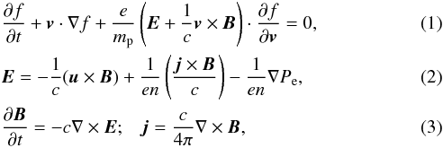 where f is the proton distribution function, E and B the electric and magnetic fields, respectively, j the total current density (the displacement current has been neglected in the Ampere equation and quasi-neutrality is assumed), mp and e are the proton mass and charge, respectively, and c is the velocity of light. The proton density n (which is equal to the electron density) and bulk velocity u are obtained as velocity moments of f. The scalar electron pressure Pe is assigned through an isothermal equation of state Pe = κBnTe, where Te = const is the electron temperature and κB the Boltzmann constant. The above equations can be re-written in a dimensionless form using the following standard procedure. We consider a typical value
  of the magnetic field and a typical density
  . Using these quantities we build up a typical Alfvén velocity
  , a gyration frequency
  , a typical proton inertial length
  , a typical current density
  , and a typical temperature
  . Then, we normalize the electric and magnetic fields E and B to ; the velocities v and u to
  ; the density n to ; the current density j to
  ; the electron temperature Te to
  ; the space variables to
  and time to
  . Equations (1)–(3) are written in terms of the dimensionless quantities defined above in the following form:
 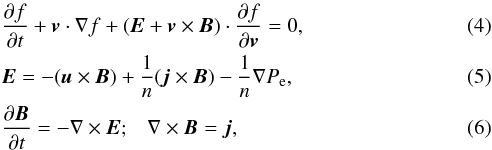 where, for simplicity, each dimensionless quantity is indicated using the same notation as the corresponding physical quantity. In what follows, all the results are expressed in terms of the dimensionless quantities defined above.
The normalized HVM Eqs. (4)–(6) have been solved in a double periodic spatial domain D = L × L = [0,16π] × [0,16π]. In the three-dimensional velocity box, the distribution function f is set equal to zero for | v | >vmax = 5vthp in each velocity direction. Physical space is discretized with Nx = 256 grid points in the x direction and Ny = 1024 gridpoints in the y direction, while velocity space with NVx = NVy = NVz = 51 grid points.
When dealing with nonuniform situations in kinetic regime, the definition of an equilibrium state is a delicate point (Cerri et al. 2013, 2014). Here, we consider a nonuniform equilibrium configuration, where physical quantities vary only along the y direction, or are uniform. Quantities relative to the equilibrium state are indicated by the upper index “(0)”. The equilibrium magnetic field is directed along the x direction:  (7)where ex is the unit vector in the x direction, while the equilibrium proton distribution function is a Maxwellian with the following form:
  (8)where the function n(0)(y) represents the nonuniform density:
  (9)and
  is the equilibrium proton temperature which we assume to be uniform. Moreover, the corresponding equilibrium proton bulk velocity is vanishing:
  (10)From Eq. (5) and using Eqs. (7) and (10), the equilibrium electric field can be derived:
 ![Mathematical equation: \begin{equation} \label{E0} {\vec E}^{(0)}=-\frac{1}{n^{(0)}(y)} \left\{ \left[ \frac{\rm d}{{\rm d} y} \left( \frac{{B^{(0)}}^2}{2} \right)\right] + \frac{{\rm d} n^{(0)}}{{\rm d}y} T_{\rm e} \right\} {\vec e}_y , \end{equation}](/articles/aa/full_html/2017/03/aa29240-16/aa29240-16-eq60.png) (11)where ey is the unit vector in the y direction. We note that ∇ × E(0) = 0; thus, according to the Faraday law Eq. (6), the magnetic field B(0) remains constant in time. Finally, we consider the Vlasov equation, calculating the single terms in Eq. (4):
(11)where ey is the unit vector in the y direction. We note that ∇ × E(0) = 0; thus, according to the Faraday law Eq. (6), the magnetic field B(0) remains constant in time. Finally, we consider the Vlasov equation, calculating the single terms in Eq. (4):  (12)
(12)![Mathematical equation: \begin{eqnarray} \label{term2} &&{\vec E}^{(0)} \cdot \frac{\partial f^{(0)}}{\partial {\vec v}} = \left[ \frac{{\rm d}}{{\rm d}y} \left( \frac{{B^{(0)}}^2}{2} \right) + T_{\rm e} \frac{{\rm d} n^{(0)}}{{\rm d}y}\right] \frac{f^{(0)}}{n^{(0)}} \frac{v_y}{T_{\rm p}^{(0)}} ,\\&&\label{term3} \left( {\vec v}\times {\vec B}^{(0)}\right) \cdot \frac{\partial f^{(0)}}{\partial {\vec v}}= \frac{B^{(0)}\, f^{(0)}}{T_{\rm p}^{(0)}} \left( v_z v_y - v_y v_z \right) = 0 . \end{eqnarray}](/articles/aa/full_html/2017/03/aa29240-16/aa29240-16-eq65.png) Using Eqs. (12)–(14), then Eq. (4) gives:
Using Eqs. (12)–(14), then Eq. (4) gives: ![Mathematical equation: \begin{equation} \label{vlasov0} \frac{\partial f^{(0)}}{\partial t} + \frac{v_y f^{(0)}}{n^{(0)} T_{\rm p}^{(0)}} \frac{\partial}{\partial y} \left[ n^{(0)} \left( T_{\rm p}^{(0)} + T_{\rm e} \right) + \frac{{B^{(0)}}^2}{2} \right] = 0 . \end{equation}](/articles/aa/full_html/2017/03/aa29240-16/aa29240-16-eq66.png) (15)Then, the proton distribution function f(0) remains stationary if the total (proton + electron + magnetic) pressure is uniform:
(15)Then, the proton distribution function f(0) remains stationary if the total (proton + electron + magnetic) pressure is uniform:  (16)In conclusion, the considered configuration represents an equilibrium state, provided that the pressure balance condition (16) is satisfied. We note that such a state also corresponds to a MHD equilibrium: in fact, since the magnetic tension associated to B(0) is vanishing (Eq. (7)), the condition (16) expresses the equilibrium among all the forces acting on the magnetofluid.
More specifically, for the equilibrium magnetic field we used the following form:  (17)which defines a magnetic field which is maximum at the center y = 8π of the domain and minimum at the borders y = 0 and y = 16π. We used the values r = 10 and h = 0.2, which give an almost homogenous field both in the central part and in the two lateral regions of the domain; these homogeneity regions are separated by two sharp shear layers which are located at approximately y = 4π and y = 12π, respectively. The last term in Eq. (17) is a small correction which has been introduced in order to acquire the null first derivative of B(0)(y) at y = 0 and y = 16π. This is obtained using the following value for the parameter α:
 ![Mathematical equation: \begin{equation} \label{alpha} \alpha=\frac{(b_M-b_m)r}{2 (2h)^r \left[1+\left(\displaystyle{\frac{1}{2h}}\right)^r \right]^2} \simeq 2.62 \times 10^{-4} . \end{equation}](/articles/aa/full_html/2017/03/aa29240-16/aa29240-16-eq79.png) (18)In this case, both B(0)(y) and dB(0)/ dy are periodic functions in the interval [ 0,16π]. However, higher order derivatives of B(0)(y) are not exactly periodic. For this reason, the expression of B(0) in Eq. (17) has been corrected by filtering out harmonics with wavenumbers larger than 70 in its spectrum. This filtering procedure does not alter the profile B(0)(y). The maximum value of B(0)(y) is given by the parameter bM = B(0)(y = 8π), while the minimum is B(0)(y = 0) = B(0)(y = 16π) ≃ bm. We performed three runs (RUN I, RUN II and RUN III) with different values of the parameters bM and bm, which are given in Table 1. In the three runs, the jump in the magnetic field magnitude through the shear regions is the same, while in RUN I values of both bM and bm larger than in RUN II and RUN III have been used.
(18)In this case, both B(0)(y) and dB(0)/ dy are periodic functions in the interval [ 0,16π]. However, higher order derivatives of B(0)(y) are not exactly periodic. For this reason, the expression of B(0) in Eq. (17) has been corrected by filtering out harmonics with wavenumbers larger than 70 in its spectrum. This filtering procedure does not alter the profile B(0)(y). The maximum value of B(0)(y) is given by the parameter bM = B(0)(y = 8π), while the minimum is B(0)(y = 0) = B(0)(y = 16π) ≃ bm. We performed three runs (RUN I, RUN II and RUN III) with different values of the parameters bM and bm, which are given in Table 1. In the three runs, the jump in the magnetic field magnitude through the shear regions is the same, while in RUN I values of both bM and bm larger than in RUN II and RUN III have been used.
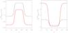 |
Fig. 1 Profiles of |

The proton equilibrium temperature is assumed to be equal to the electron temperature  . The equilibrium density n(0)(y) has been determined by imposing the total pressure equilibrium (16):
  (19)The values of the total pressure
  and of the temperature T(0), which have been used for the three runs, are given in Table 1. The condition (19) ensures that the considered equilibrium is a stationary state of the system. This has been explicitly verified by performing a run (not shown) in which the above equilibrium state is used as the initial condition.
We define a non uniform Alfvén velocity associated with the equilibrium structure as  and a non uniform proton plasma beta at equilibrium as
  . In Fig. 1 the profiles of
  (left panel) and
  (right panel) are shown for RUN I (black curve) and for RUN II and RUN III (red curve): the shear layers and the homogeneity regions are clearly visible, where
  have values either larger or smaller than the unity.
Simulations setup.
At the initial time t = 0 a linearly polarized Alfvénic perturbation is superposed on the above-defined equilibrium. The initial value of the magnetic field (equilibrium + perturbation) is  (20)with ez the unit vector in the z direction, and a the amplitude of the initial perturbation. The initial proton distribution function is a shifted Maxwellian of the following form
 ![Mathematical equation: \begin{equation} \label{ft0} f(x,y,{\vec v},t=0) = \frac{n^{(0)}(y)}{(2\pi T^{(0)})^{3/2}} \exp \! \left\{ -\frac{v_x^2+v_y^2+\left[ v_z-u^{(1)}(x,y)\right]^2}{2T^{(0)}}\right\} , \end{equation}](/articles/aa/full_html/2017/03/aa29240-16/aa29240-16-eq104.png) (21)where
(21)where ![Mathematical equation: \begin{equation} u^{(1)}(x,y)=-\frac{a}{\left[ n^{(0)}(y)\right]^{-1/2}} \cos (x/8) . \end{equation}](/articles/aa/full_html/2017/03/aa29240-16/aa29240-16-eq105.png) (22)It can be verified that the density and temperature associated with the initial proton distribution function (21) are, respectively:
(22)It can be verified that the density and temperature associated with the initial proton distribution function (21) are, respectively:  (23)indicating that the initial density and temperature perturbations are both vanishing. Moreover, the initial proton bulk velocity is
 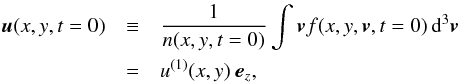 (24)so that
 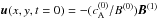 . The values of the perturbation amplitude a are given in Table 1.
In the three runs, both the equilibrium structure and the perturbation amplitude are modified, so as to increase the level of nonlinearity when going from RUN I to RUN III. In fact, in RUN II the perturbation amplitude does not change with respect to RUN I, but the average equilibrium magnetic field intensity is smaller than in RUN I, implying a larger ratio a/B(0)(y). Then, we expect that nonlinear effects are more relevant in RUN II than in RUN I. In particular, nonlinearities are more relevant in the lateral regions of D, where B(0) has lower values. Nonlinear effects further increase in RUN III, where the perturbation amplitude is increased by a factor 1.5, while the same equilibrium as in RUN II is considered. Finally, we note that the profiles of are different for the three runs, the configuration of RUN II and RUN III corresponding to a mean larger than in RUN I.
3. Results
As recently discussed in Vásconez et al. (2015), Pucci et al. (2016), when initializing the HVM simulations with the configuration described above, the mechanism of phase-mixing of large-scale parallel propagating Alfvén waves in the shear regions produces KAW fluctuations at wavelengths close to dp and at large propagation angles with respect to the magnetic field. These perturbations, while propagating in the x direction, drift along y towards the boundaries of the simulation box, due to a non-vanishing transverse component of the group velocity. Here, we present a detailed study of the role of kinetic effects on protons associated with the propagation of KAWs produced by the above mechanism, as dependent on the characteristic of the initial equilibrium and/or on the amplitude of the initial Alfvénic perturbation. In particular, we focus on the deviations of the proton VDF from thermodynamic equilibrium and report on the transition to a turbulent state observed when increasing the amplitude of the initial disturbance as compared to the background values.
In order to characterize and compare the three runs, we have computed the quantity ϵ(x,y,t) (Greco et al. 2012), which is a measure of the deviation of the proton VDF from the Maxwellian configuration shape: ![Mathematical equation: \begin{equation} \epsilon(x,y,t)=\frac{1}{n({\vec x},t)} \sqrt{\int \left[f({\vec x}, {\vec v}, t) - M({\vec x}, {\vec v}, t)\right]^2{\rm d}^3v}. \end{equation}](/articles/aa/full_html/2017/03/aa29240-16/aa29240-16-eq112.png) (25)Here, M is the corresponding Maxwellian distribution with the same density, bulk velocity and isotropic temperature as f; ϵ is a positive definite quantity and may be viewed as a distance or separation between the computed f and an equivalent Maxwellian. Figure 2 shows the time evolution of ϵmax(t) = maxD { ϵ(x,y,t) } (the maximum value of ϵ over the two-dimensional domain D), from the simulations as in Table 1. From this figure it can be seen that ϵmax grows in time for all simulations reaching an almost constant saturation value after the time td ≃ 60, that gives an estimation of the typical time at which phase mixing produces transverse scales of the order of dp (Vásconez et al. 2015). It is clear from this picture that the saturation level of ϵmax increases as the initial perturbation amplitude to the mean equilibrium magnetic field intensity ratio increases. In fact, going from RUN I, through RUN II, to RUN III, nonlinear effects become more and more relevant, and kinetic processes work more and more efficiently to drive the protons away from thermodynamic equilibrium.
(25)Here, M is the corresponding Maxwellian distribution with the same density, bulk velocity and isotropic temperature as f; ϵ is a positive definite quantity and may be viewed as a distance or separation between the computed f and an equivalent Maxwellian. Figure 2 shows the time evolution of ϵmax(t) = maxD { ϵ(x,y,t) } (the maximum value of ϵ over the two-dimensional domain D), from the simulations as in Table 1. From this figure it can be seen that ϵmax grows in time for all simulations reaching an almost constant saturation value after the time td ≃ 60, that gives an estimation of the typical time at which phase mixing produces transverse scales of the order of dp (Vásconez et al. 2015). It is clear from this picture that the saturation level of ϵmax increases as the initial perturbation amplitude to the mean equilibrium magnetic field intensity ratio increases. In fact, going from RUN I, through RUN II, to RUN III, nonlinear effects become more and more relevant, and kinetic processes work more and more efficiently to drive the protons away from thermodynamic equilibrium.
 |
Fig. 2 Time evolution of the parameter ϵmax (detailed in the text) computed from the VDFs of RUN I (black triangles), RUN II (green diamonds) and RUN III (red stars). The vertical blue-dashed line corresponds to the theoretical estimation of the time at which phase-mixing produces transverse scales comparable to dp. |
The subsequent analysis of the system has been performed at a given time (t = t∗ = 105), at which ϵmax has reached its saturation level for all the runs and kinetic processes have significantly influenced the proton dynamics. In Fig. 3, the contour plots of | j | (upper row), ϵ (middle row) and δT = T−T(0) (lower row) are reported for RUN I (left column), RUN II (central column) and RUN III (right column). Going from RUN I to RUN III, the current density, originally concentrated near the shear regions (panel a), becomes more intense and tends to filament when kinetic physics becomes dominant (panel c). Non-Maxwellian features in RUN I are essentially located within the shear regions near the peaks of | j | (panel d). In RUN II, such features are still peaked in the shear regions where dispersive effects responsible for the KAW formation are active (panel e). However, significant departures from Maxwellianity are visible also in the lateral homogeneous regions, starting from the early stage of the simulation (not shown). This becomes more evident in RUN III (panel f). These latter features can be ascribed to nonlinear effects, which are particularly strong in the lateral regions, where the ratio a/B(0) is of the order of unity. Finally, temperature variations also exhibit a behavior similar to that of ϵ, being more intense in the shear regions for RUN I (panel g) as compared to RUN II (panel h) and RUN III (panel i), in which significant values of δT are recovered in the whole spatial domain.
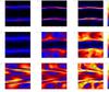 |
Fig. 3 2D contour plots, at t = 105, of the modulus of the current density | j | (upper row), the non-Maxwellianity measure ϵ (middle row), and temperature variations δT (lower row), for RUN I (left column), RUN II (middle column), and RUN III (right column). |
We also noticed that, when increasing the nonlinearity of the initial perturbation, a clear transition to turbulence is recovered. This can be appreciated in Fig. 4 where the power spectra of magnetic | δBk | 2 (top) and electric | δEk | 2 (middle) energy, summed over the parallel wavenumbers kx (reduced spectra), are plotted as a function of the transverse wavenumber ky. Here, for each field g(x,y), we have computed δg(x,y) = g(x,y)−⟨g(x,y)⟩x, where ⟨·⟩x represents the mean value in the x direction. It is clear from these plots that the magnetic and electric energy content at wavenumbers larger than kydp ≃ 2 is negligible for the case of RUN I (black curve), while it increases significantly for RUN II and RUN III (green and red curve, respectively). Moreover, at the bottom of same figure, we display the power spectrum of the parallel electric energy | δE∥ k | 2. Here, the clear peak visible at kydp ≃ 2 in the case of RUN I (black curve) corresponds to the KAW fluctuations produced through phase mixing, as discussed in detail in (Vásconez et al. 2015). It is worth noticing that this peak disappears with increasing spectrum extension (green and red curves), meaning that the energy stored in KAW fluctuations cascades towards short spatial scales when kinetic processes come into play.
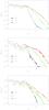 |
Fig. 4 Power spectra of the total magnetic field (top panel), total electric field (middle panel) and electric field component parallel to the local magnetic field (bottom panel), for RUN I (black line), RUN II (green line) and RUN III (red line). |
We point out that the final state reached in RUN III is not a state of fully developed turbulence in the classical Kolmogorov view, but that it can be thought of as a state of increased nonlinearity, with respect to RUN I and RUN II; in fact, going from RUN I to RUN III the signature of wave-like activity (the well-defined bump visible in the spectra for RUN I) is gradually lost and a significant amount of energy reaches the spectral range of high wavenumbers.
The Eulerian HVM code allows for an almost noise-free description of the proton distribution function in phase space, making it, for this reason, an indispensable tool for analyzing the effects of kinetic processes on plasma dynamics. In Fig. 5, we report the three-dimensional surface plots of the proton VDF at t = 105, computed at the spatial point where ϵ = ϵmax for each run (these spatial points are located inside the shear regions, as can be seen in the middle panels of Fig. 3). The unit vector of the local magnetic field is displayed in these plots as a magenta tube. In the upper plot, corresponding to RUN I, one notices smooth deviations of the particle VDF from the spherical Maxwellian shape, with the appearance of a barely visible bulge along the local field and a ring-like modulation in the perpendicular plane. Here, the direction of the local field appears to still be a preferred direction of symmetry for the particle VDF. In RUN II (middle plot) where nonlinearities are stronger, the particle VDF appears more distorted than in RUN I. Finally, in RUN III (lower plot) where the transition to a turbulent state has been observed through the power spectra discussed above, any symmetry of the VDF is lost, as sharp gradients and small-scale velocity structures have been produced through the nonlinear interaction of protons with the fluctuating fields.
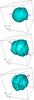 |
Fig. 5 Iso-surface plot of the proton VDF in velocity space, at the spatial location where ϵ is maximum for RUN I (top), RUN II (middle), and RUN III (bottom); the magenta tube in each plot indicates the direction of the local magnetic field. |
In order to provide a more quantitative description of the deviation of the VDFs from thermodynamic equilibrium, we computed the preferred directions of f in velocity space (Servidio et al. 2012), for each spatial position, from the stress tensor: 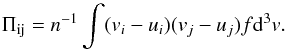 (26)This tensor can be diagonalized by computing its eigenvalues { λ1,λ2,λ3 } (ordered in such way that λ1>λ2>λ3) and the corresponding normalized eigenvectors
  which define the minimum variance frame (MVF). We point out that λi are the temperatures and
  the anisotropy directions of the VDF. The information given by the ratios λi/λj is in some sense included in ϵ; nevertheless, the ratios of the eigenvalues evidently provide additional relevant insights into the symmetry of VDF, which is important to investigate. Therefore, for RUN III at t = t∗ = 105, we computed the probability distribution function (PDF) of the ratios λi/λj (i,j = 1,2,3 and j ≠ i), conditioned to the values of ϵ(t = t∗). Note that each of these ratios is equal to unity for a Maxwellian VDF. In Fig. 6, we show the PDF of λ1/λ2 (left panel), λ1/λ3 (middle panel) and λ2/λ3 (right panel); these PDFs have been computed for three different ranges of values of ϵ, 0 ≤ ϵ(t∗) ≤ ϵmax(t∗) / 3 (black curve), ϵmax(t∗) / 3 <ϵ(t∗) ≤ 2ϵmax(t∗) / 3 (red curve) and 2ϵmax(t∗) / 3 ≤ ϵ(t∗) ≤ ϵmax(t∗) (blue curve). It can be noticed from this figure that in the range of small ϵ the three PDFs have a peak close to unity (they are not exactly centered around 1, since the minimum value of ϵ is not zero), suggesting that, when the level of nonlinearity is low, the distribution function can be slightly far from the Maxwellian shape, still keeping one (or more) axis of symmetry. On the other hand, as ϵ increases, high tails appear in the PDF signals, meaning that in the case of significant deviations from Maxwellian, is not possible to make assumptions on the shape of the VDF. As a consequence, the use of reduced models, based on restrictive approximations on the symmetry of the VDF, is not appropriate and one must adopt more complete models able to describe the evolution of the VDF in a full 3D velocity space. Note, in particular, that because of the multiple anisotropies observed, and because of the misalignment with the ambient field, any gyrotropic approximation loses its validity, as we further demonstrate below. We point out that our hybrid model is limited by the fluid approximation used for the electrons. Recent high-resolution measurements in the magnetosheath plasma (Burch et al. 2016) show that the velocity distributions of electrons display marked non fluid behavior. For these reasons, we expect that a full treatment including kinetic electrons would reveal a dynamics analogous to that of the protons, with even more pronounced non-thermal effects, especially close to reconnecting current sheets.
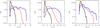 |
Fig. 6 PDF of λ1/λ2 (left), λ1/λ3 (middle) and λ2/λ3 (right) from RUN III at t = 105, computed for three different ranges of values of ϵ, namely 0 ≤ ϵ(t∗) ≤ ϵmax(t∗) / 3 (black curve), ϵmax(t∗) / 3 <ϵ(t∗) ≤ 2ϵmax(t∗) / 3 (red curve) and 2ϵmax(t∗) / 3 ≤ ϵ(t∗) ≤ ϵmax(t∗) (blue curve). |
With the aim of characterizing the nature of the deformation of the particle VDFs and to identify the spatial regions that are the sites of kinetic activity, we computed two indexes of departure from Maxwellian, that is, the temperature anisotropy index and the gyrotropy index, in two different reference frames; namely the MVF and the local magnetic field frame (LMF). Therefore, we define the anisotropy indicators ζ = | 1−λ1/λ3 | (MVF) and ζ∗ = | 1−T⊥/T∥ | (LMF), where T⊥ and T∥ are the temperatures with respect to the local magnetic field, and the gyrotropy indicator in the MVF η = | 1−λ2/λ3 |. The gyrotropy indicator in the LMF η∗ can be computed by using the normalized Frobenius norm of the non-gyrotropic part N of the full pressure tensor Π, introduced by Aunai et al. (2013):  (27)where Nij are the components of the tensor N, and Tr(N) = 0. It is worth pointing out that all indexes defined above are identically null if the particle VDF is Maxwellian. The contour plots of ϵ in the middle column of Fig. 3 show that the main departures from Maxwellian occur, for both runs, in the shear regions where current density achieves its maximum value (though high values of ϵ are spread on a larger portion of the spatial domain around the shear regions for RUN II and even more for RUN III). In Fig. 7 we report the y profile of the non-Maxwellianity indexes ζ (anisotropy in the MVF), ζ∗ (anisotropy in the LMF), η (non-gyrotropy in the MVF) and η∗ (non-gyrotropy in the LMF), averaged over x for the three runs. We focus on the shear region on the upper half of the spatial simulation domain (delimited by vertical black-dashed lines).
In the more turbulent situation of RUN III, nonlinear interaction of protons with large amplitude fluctuations of the KAW type generates larger deviation of the particle VDF from Maxwellian in the shear region. Moreover, this effect is also visible in the regions outside the shear; this could be due to both the transverse drift of KAWs from the shear regions towards the boundaries of the numerical domain (Vásconez et al. 2015), and to nonlinear effects intrinsic to the initial perturbations which are stronger in such lateral regions. On the other hand, for the quasi-linear RUN I, the particle VDF becomes anisotropic and non-gyrotropic as viewed from both MVF and LMF, only in the shear regions. An intermediate situation is observed for RUN II.
In order to quantitatively study the generation of structures in velocity space due to kinetic processes, we implemented the following procedure. We again focused on the most turbulent run (RUN III) at time t = t∗ = 105. We selected the spatial locations where the maximum and the minimum values of ϵ are achieved at this time and considered the corresponding proton VDFs fmax(v) and fmin(v) at these spatial locations. It is worth noting that fmax(v) is the VDF shown in Fig. 5 (bottom). Therefore, we performed a rotation of fmax(v) and fmin(v), moving them into the system v′ in which the local magnetic field is along the  direction. At this point, we computed the quantities
  and
and  ,
,  being the bi-Maxwellian VDF evaluated through the velocity moments of fmax / min. We remark that δmax and δmin store information about the kinetic effects at work in the system evolution, since, by subtracting their corresponding bi-Maxwellian from the VDFs, the main fluid-like effects have been ruled out. Note that there are several recent works where attention has been concentrated on the dynamics of the velocity space, very often invoked as entropy cascade (Tatsuno et al. 2009; Howes et al. 2011; Schekochihin et al. 2016). This new concept is very interesting since it connects the cascade in physical space with a similar cascade in velocity space, where finer and finer scales are formed and finally dissipated through Landau damping or collisional mechanisms (Pezzi et al. 2016).
In order to analyze the velocity space structures, one can proceed in several ways. One possibility is given by the decomposition of the VDF through Hermite polynomials (Tatsuno et al. 2009; Howes et al. 2011; Schekochihin et al. 2016; Pezzi et al. 2016). The advantage of this complete decomposition is that one can capture all the features in velocity space (especially in our case, where high resolution VDFs are available). On the other hand the interpretation of the eigenmodes in terms of classical scaling arguments (in analogy with the cascade in physical space) may be quite complicated in a case where the VDF is fully three-dimensional and cannot be reduced to a simplified system by assuming, for example, gyrotropy. The second possibility is to decompose the fluctuations using classical Fourier decomposition in order to measure the intensity of the velocity space fluctuations and understanding typical scales in velocity space. Even though δmax and δmin are not formally periodic functions in velocity space, they go rapidly to zero at the boundary of the simulation velocity box, allowing, therefore, the use of Fast Fourier transforms. For this reason, in order to characterize the velocity space structures generated by the kinetic dynamics of protons, we performed a velocity space Fourier transformation of δmax and δmin. In Fig. 8, we show the Fourier spectra  (averaged over
  and
and  , left),
  (averaged over
  and , middle) and
  (averaged over and , right), respectively, for δmax (black line) and δmin (red line). Here,
  represents the velocity space wave number associated with the velocity scale
  .
.
One can easily see that, in each direction, velocity space spectra of δmin (VDF close to the Maxwellian shape) display a significantly lower power amplitude than those of δmax. Moreover, since the spectra of δmax (black curves) have comparable energetic content in each direction, one may argue that there is no preferential direction for the VDF, when this is efficiently shaped by kinetic processes. In particular, the high kv bumps may indicate the presence of structures (beams and rings) in velocity space. An interesting analogy arises here with the cascade in physical space, in the presence of strongly anisotropic turbulence. As can be observed from Fig. 8, for a low level of kinetic activity (red curves), some isolated high-kv peaks can be observed, possibly related to local Cherenkov and/or cyclotron resonances (Kennel & Englelmann 1966). These are similar to the peaks observed due to wave activity in the Eulerian spectra (Dmitruk & Matthaeus 2009). On the other hand, when the level of kinetic activity increases (black curves), these peaks disappear, and a more continuum cascade-like spectrum is observed in velocity space, similarly to that recovered in physical space (cf. with Fig. 4). This is a preliminary study, which surely deserves a future investigation. This phenomenology could be related to the idea of the “double cascade” (physical-velocity space), as suggested in several recent works (Tatsuno et al. 2009; Schekochihin et al. 2016).
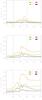 |
Fig. 7 Anisotropy indexes ζ (orange line) and ζ∗ (green line) and non-gyrotropy indexes η (red line), and η∗ (black line), averaged over x and plotted as a function of y in the interval y = [L/ 2,L], for RUN I (top panel), RUN II (middle panel) and RUN III (bottom panel). |
4. Summary and conclusions
As recently shown by Vásconez et al. (2015), Pucci et al. (2016), kinetic Alfvén waves are naturally generated through the phase mixing mechanism, when Alfvén waves propagate in an inhomogeneous medium. In the present paper, we numerically reproduced the generation of KAWs through 2D-3V Hybrid Vlasov-Maxwell simulations by imposing Alfvénic perturbations on an initial pressure balanced magnetic shear equilibrium. Both the characteristics of the initial equilibrium and the amplitude of the perturbations have been varied in order to explore the system dynamics in different regimes, focusing, in particular, on the transition from a quasi-linear to a turbulent regime. Moreover, as the HVM code provides an almost noise-free description of the proton distribution function, we have shown how the interaction of large amplitude KAW fluctuations with protons shapes the VDF and makes it depart from local thermodynamic equilibrium.
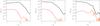 |
Fig. 8 One-dimensional velocity space Fourier spectra |
When comparing the quasi-linear RUN I with the more nonlinear RUN II and the turbulent RUN III, one realizes that many interesting effects arise as the amplitude of the perturbations increases and the gradients of the initial magnetic shear become sharper. First of all, any wave-like activity, recognized in RUN I as well-defined bumps in the turbulent electric and magnetic spectra, disappears in RUN II and RUN III, in which a significant amount of energy is recovered at short spatial scales. As a consequence of this small-scale activity, the proton VDF appears much more distorted in RUN III as compared to RUN I, losing any property of symmetry with respect to the direction of the local magnetic field. Indeed, as discussed in detail in the previous section, in RUN III, in the spatial regions where strong departures from Maxwellian are observed, the proton VDF develops temperature anisotropy, non-gyrotropy features and many other complicated deformations.
We proposed to provide quantitative information on these kinetic distortions of the proton VDF by employing different non-Maxwellianity indexes such as the anisotropy index and the non-gyrotropy index, which have been computed both in the minimum variance frame and in the local magnetic field frame. Interestingly, all these indexes behave in a similar way, achieving higher values in the shear regions, where the initial magnetic configuration produced strong current sheets, while decreasing in the homogeneous regions far from the shears. These results support the idea (Servidio et al. 2012; Valentini et al. 2014) that proton kinetic effects are not uniformly distributed in space, but are rather intermittent and localized in certain space regions determined by the topology of the magnetic field. In future works, we plan to extend our numerical studies to include the kinetic physics of electrons, which are expected to reveal a stronger non-Maxwellian character.
Finally, through a Fourier analysis performed on the deviations of the proton VDF from a bi-Maxwellian, we pointed out that, when kinetic effects are retained in the description of the plasma dynamics, beside a turbulent cascade in physical space, an analogous cascade is produced in velocity space (Tatsuno et al. 2009; Howes et al. 2011; Schekochihin et al. 2016), thus emphasizing the physical link between the small spatial scale structures driven by the turbulent cascade and the fine velocity gradients naturally arising through kinetic effects.
Acknowledgments
This work has been supported by the Agenzia Spaziale Italiana under the Contract No. ASI-INAF 2015-039-R.O “Missione M4 di ESA: Partecipazione Italiana alla fase di assessment della missione THOR”. The numerical HVM simulations were run on the Fermi supercomputer at CINECA (Bologna, Italy), within the ISCRA-C projects IsC26-COLTURBO, IsC26-PMKAW and IsC25-MHDwMoPC.
References
- Aunai, N., Hesse, M., & Kuznetsova, M. 2013, Phys. Plasmas, 20, 092903 [NASA ADS] [CrossRef] [Google Scholar]
- Bale, S., Kellogg, P., Mozer, F., Horbury, T., & Reme, H. 2005, Phys. Rev. Lett., 94, 215002 [NASA ADS] [CrossRef] [PubMed] [Google Scholar]
- Belcher, J., & Davis, L. 1971, J. Geophys. Res., 76, 3534 [NASA ADS] [CrossRef] [Google Scholar]
- Bruno, R., & Carbone, V. 2013, Liv. Rev. Sol. Phys., 10, 2 [Google Scholar]
- Burch, J. L., Torbert, R. B., Phan, T. D., et al. 2016, Science, 352, 6290 [Google Scholar]
- Califano, F., Chiuderi, C., & Einaudi, G. 1990, ApJ, 365, 757 [NASA ADS] [CrossRef] [Google Scholar]
- Califano, F., Chiuderi, C., & Einaudi, G. 1992, ApJ, 390, 560 [NASA ADS] [CrossRef] [Google Scholar]
- Carbone, V., & Veltri, P. 1990, Geophys. Astrophys. Fluid Dyn., 52, 153 [NASA ADS] [CrossRef] [Google Scholar]
- Cerri, S. S., Henri, P., Califano, F., et al. 2013, Phys. Plasmas, 20, 112112 [NASA ADS] [CrossRef] [Google Scholar]
- Cerri, S. S., Pegoraro, F., Califano, F., Del Sarto, D., & Jenko, F. 2014, Phys. Plasmas, 21, 112109 [Google Scholar]
- Chen, C., Boldyrev, S., Xia, Q., & Perez, J. 2013, Phys. Rev. Lett., 110, 225002 [NASA ADS] [CrossRef] [Google Scholar]
- Davila, J. M. 1987, ApJ, 317, 514 [NASA ADS] [CrossRef] [Google Scholar]
- Décamp, N., & Malara, F. 2006, in SOHO-17. 10 Years of SOHO and Beyond, Proc. Conf. ESA SP, 617, 26 [NASA ADS] [Google Scholar]
- Dmitruk, P., & Matthaeus, W. 2009, Phys. Plasmas, 16, 062304 [NASA ADS] [CrossRef] [Google Scholar]
- Gary, S. P., & Nishimura, K. 2004, J. Geophys. Res.: Space Phys., 109, A02109 [NASA ADS] [CrossRef] [Google Scholar]
- Ghosh, S., Matthaeus, W., Roberts, D., & Goldstein, M. 1998, J. Geophys. Res.: Space Phys., 103, 23691 [NASA ADS] [CrossRef] [Google Scholar]
- Greco, A., Valentini, F., Servidio, S., & Matthaeus, W. 2012, Phys. Rev. E, 86, 066405 [NASA ADS] [CrossRef] [Google Scholar]
- Heyvaerts, J., & Priest, E. 1983, A&A, 117, 220 [NASA ADS] [Google Scholar]
- Hollweg, J. V. 1987, ApJ, 312, 880 [NASA ADS] [CrossRef] [Google Scholar]
- Hollweg, J. V. 1999, J. Geophys. Res.: Space Phys., 104, 14811 [Google Scholar]
- Howes, G., Dorland, W., Cowley, S., et al. 2008a, Phys. Rev. Lett., 100, 065004 [NASA ADS] [CrossRef] [Google Scholar]
- Howes, G. G., Cowley, S. C., Dorland, W., et al. 2008b, J. Geophys. Res.: Space Phys., 113, A05103 [NASA ADS] [CrossRef] [Google Scholar]
- Howes, G. G., TenBarge, J. M., Dorland, W., et al. 2011, Phys. Rev. Lett., 107, 035004 [NASA ADS] [CrossRef] [PubMed] [Google Scholar]
- Kaghashvili, E. K. 1999, ApJ, 512, 969 [NASA ADS] [CrossRef] [Google Scholar]
- Kennel, C. F., & Engelmann, F. 1966, Phys. Fluids, 8, 2377 [NASA ADS] [CrossRef] [Google Scholar]
- Kiyani, K. H., Chapman, S. C., Sahraoui, F., et al. 2013, ApJ, 763, 10 [NASA ADS] [CrossRef] [Google Scholar]
- Landi, S., Velli, M., & Einaudi, G. 2005, ApJ, 624, 392 [NASA ADS] [CrossRef] [Google Scholar]
- Lee, M., & Roberts, B. 1986, ApJ, 301, 430 [NASA ADS] [CrossRef] [Google Scholar]
- Lysak, R. L., & Song, Y. 2011, J. Geophys. Res.: Space Phys., 116, A00K14 [CrossRef] [Google Scholar]
- Malara, F., Veltri, P., Chiuderi, C., & Einaudi, G. 1992, ApJ, 396, 297 [NASA ADS] [CrossRef] [Google Scholar]
- Malara, F., Primavera, L., & Veltri, P. 1996, ApJ, 459, 347 [NASA ADS] [CrossRef] [Google Scholar]
- Malara, F., Petkaki, P., & Veltri, P. 2000, ApJ, 533, 523 [NASA ADS] [CrossRef] [Google Scholar]
- Malara, F., De Franceschis, M., & Veltri, P. 2003, A&A, 412, 529 [NASA ADS] [CrossRef] [EDP Sciences] [Google Scholar]
- Malara, F., De Franceschis, M., & Veltri, P. 2005, A&A, 443, 1033 [NASA ADS] [CrossRef] [EDP Sciences] [Google Scholar]
- Malara, F., Veltri, P., & De Franceschis, M. 2007, A&A, 467, 1275 [NASA ADS] [CrossRef] [EDP Sciences] [Google Scholar]
- Matthaeus, W., Goldstein, M., & King, J. 1986, J. Geophys. Res.: Space Phys., 91, 59 [NASA ADS] [CrossRef] [Google Scholar]
- Matthaeus, W. H., Goldstein, M. L., & Roberts, D. A. 1990, J. Geophys. Res., 95, 673 [Google Scholar]
- McLaughlin, J., Hood, A., & De Moortel, I. 2011, Space Sci. Rev., 158, 205 [NASA ADS] [CrossRef] [Google Scholar]
- Mok, Y., & Einaudi, G. 1985, J. Plasma Phys., 33, 199 [NASA ADS] [CrossRef] [Google Scholar]
- Nakariakov, V., Roberts, B., & Murawski, K. 1997, Sol. Phys., 175, 93 [NASA ADS] [CrossRef] [Google Scholar]
- Ofman, L. 2010, J. Geophys. Res.: Space Phys., 115, 04108 [Google Scholar]
- Ofman, L., & Aschwanden, M. 2002, ApJ, 576, L153 [NASA ADS] [CrossRef] [Google Scholar]
- Oughton, S., Priest, E. R., & Matthaeus, W. H. 1994, J. Fluid Mech., 280, 95 [NASA ADS] [CrossRef] [Google Scholar]
- Ozak, N., Ofman, L., & Vinas, A. F. 2015, ApJ, 799, 77 [NASA ADS] [CrossRef] [Google Scholar]
- Petkaki, P., Malara, F., & Veltri, P. 1998, ApJ, 500, 483 [NASA ADS] [CrossRef] [Google Scholar]
- Pezzi, O., Valentini, F., & Veltri, P. 2016, Phys. Rev. Lett., 116, 145001 [NASA ADS] [CrossRef] [Google Scholar]
- Podesta, J. J., & TenBarge, J. M. 2012, J. Geophys. Res.: Space Phys., 117, 10106 [NASA ADS] [Google Scholar]
- Pucci, F., Onofri, M., & Malara, F. 2014, ApJ, 796, 43 [NASA ADS] [CrossRef] [Google Scholar]
- Pucci, F., Vasconez, C. L., Pezzi, O., et al. 2016, J. Geophys. Res.: Space Phys., 121, 1024 [NASA ADS] [CrossRef] [Google Scholar]
- Sahraoui, F., Goldstein, M., Robert, P., & Khotyaintsev, Y. V. 2009, Phys. Rev. Lett., 102, 231102 [NASA ADS] [CrossRef] [PubMed] [Google Scholar]
- Sahraoui, F., Belmont, G., & Goldstein, M. 2012, ApJ, 748, 100 [NASA ADS] [CrossRef] [Google Scholar]
- Salem, C., Howes, G., Sundkvist, D., et al. 2012, ApJ, 745, L9 [NASA ADS] [CrossRef] [Google Scholar]
- Schekochihin, A., Cowley, S., Dorland, W., et al. 2009, ApJSS, 182, 310 [NASA ADS] [CrossRef] [Google Scholar]
- Schekochihin, A. A., Parker, J. T., Highcock, E. G., et al. 2016, J. Plasma Phys., 82, 905820212 [CrossRef] [Google Scholar]
- Servidio, S., Valentini, F., Califano, F., & Veltri, P. 2012, Phys. Rev. Lett., 108, 045001 [NASA ADS] [CrossRef] [PubMed] [Google Scholar]
- Servidio, S., Osman, K., Valentini, F., et al. 2014, ApJ, 781, L27 [NASA ADS] [CrossRef] [Google Scholar]
- Servidio, S., Valentini, F., Perrone, D., et al. 2015, J. Plasma Phys., 81, 1 [CrossRef] [Google Scholar]
- Shebalin, J. V., Matthaeus, W. H., & Montgomery, D. 1983, J. Plasma Phys., 29, 525 [NASA ADS] [CrossRef] [Google Scholar]
- Similon, P. L., & Sudan, R. 1989, ApJ, 336, 442 [NASA ADS] [CrossRef] [Google Scholar]
- Steinolfson, R. 1985, ApJ, 295, 213 [NASA ADS] [CrossRef] [Google Scholar]
- Tatsuno, T., Dorland, W., Schekochihin, A., et al. 2009, Phys. Rev. Lett., 103, 015003 [NASA ADS] [CrossRef] [Google Scholar]
- TenBarge, J., & Howes, G. 2012, Phys. Plasmas, 19, 055901 [NASA ADS] [CrossRef] [Google Scholar]
- Tomczyk, S., & McIntosh, S. W. 2009, ApJ, 697, 1384 [NASA ADS] [CrossRef] [Google Scholar]
- Tomczyk, S., McIntosh, S., Keil, S., et al. 2007, Science, 317, 1192 [NASA ADS] [CrossRef] [PubMed] [Google Scholar]
- Tsiklauri, D. 2011, Phys. Plasmas, 18, 092903 [NASA ADS] [CrossRef] [Google Scholar]
- Tsiklauri, D. 2012, Phys. Plasmas, 19, 082903 [NASA ADS] [CrossRef] [Google Scholar]
- Tsiklauri, D., & Nakariakov, V. M. 2002, A&A, 393, 321 [NASA ADS] [CrossRef] [EDP Sciences] [Google Scholar]
- Tsiklauri, D., Nakariakov, V. M., & Rowlands, G. 2003, A&A, 400, 1051 [NASA ADS] [CrossRef] [EDP Sciences] [Google Scholar]
- Tsiklauri, D., Sakai, J.-I., & Saito, S. 2005, A&A, 435, 1105 [NASA ADS] [CrossRef] [EDP Sciences] [Google Scholar]
- Valentini, F., Trávníček, P., Califano, F., Hellinger, P., & Mangeney, A. 2007, J. Comput. Phys., 225, 753 [NASA ADS] [CrossRef] [Google Scholar]
- Valentini, F., Perrone, D., & Veltri, P., 2011, ApJ, 739, 54 [NASA ADS] [CrossRef] [Google Scholar]
- Valentini, F., Servidio, S., Perrone, D., et al. 2014, Phys. Plasmas, 21, 082307 [NASA ADS] [CrossRef] [Google Scholar]
- Vásconez, C. L., Valentini, F., Camporeale, E., & Veltri, P. 2014, Phys. Plasmas, 21, 112107 [NASA ADS] [CrossRef] [Google Scholar]
- Vásconez, C., Pucci, F., Valentini, F., et al. 2015, ApJ, 815, 7 [NASA ADS] [CrossRef] [Google Scholar]
- Voitenko, Y., & Goossens, M. 2004, ApJ, 605, L149 [NASA ADS] [CrossRef] [Google Scholar]
All Tables
All Figures
|
Fig. 1 Profiles of |
| In the text | |
|
Fig. 2 Time evolution of the parameter ϵmax (detailed in the text) computed from the VDFs of RUN I (black triangles), RUN II (green diamonds) and RUN III (red stars). The vertical blue-dashed line corresponds to the theoretical estimation of the time at which phase-mixing produces transverse scales comparable to dp. |
| In the text | |
|
Fig. 3 2D contour plots, at t = 105, of the modulus of the current density | j | (upper row), the non-Maxwellianity measure ϵ (middle row), and temperature variations δT (lower row), for RUN I (left column), RUN II (middle column), and RUN III (right column). |
| In the text | |
|
Fig. 4 Power spectra of the total magnetic field (top panel), total electric field (middle panel) and electric field component parallel to the local magnetic field (bottom panel), for RUN I (black line), RUN II (green line) and RUN III (red line). |
| In the text | |
|
Fig. 5 Iso-surface plot of the proton VDF in velocity space, at the spatial location where ϵ is maximum for RUN I (top), RUN II (middle), and RUN III (bottom); the magenta tube in each plot indicates the direction of the local magnetic field. |
| In the text | |
|
Fig. 6 PDF of λ1/λ2 (left), λ1/λ3 (middle) and λ2/λ3 (right) from RUN III at t = 105, computed for three different ranges of values of ϵ, namely 0 ≤ ϵ(t∗) ≤ ϵmax(t∗) / 3 (black curve), ϵmax(t∗) / 3 <ϵ(t∗) ≤ 2ϵmax(t∗) / 3 (red curve) and 2ϵmax(t∗) / 3 ≤ ϵ(t∗) ≤ ϵmax(t∗) (blue curve). |
| In the text | |
|
Fig. 7 Anisotropy indexes ζ (orange line) and ζ∗ (green line) and non-gyrotropy indexes η (red line), and η∗ (black line), averaged over x and plotted as a function of y in the interval y = [L/ 2,L], for RUN I (top panel), RUN II (middle panel) and RUN III (bottom panel). |
| In the text | |
|
Fig. 8 One-dimensional velocity space Fourier spectra |
| In the text | |
Current usage metrics show cumulative count of Article Views (full-text article views including HTML views, PDF and ePub downloads, according to the available data) and Abstracts Views on Vision4Press platform.
Data correspond to usage on the plateform after 2015. The current usage metrics is available 48-96 hours after online publication and is updated daily on week days.
Initial download of the metrics may take a while.