| Issue |
A&A
Volume 598, February 2017
|
|
|---|---|---|
| Article Number | A121 | |
| Number of page(s) | 15 | |
| Section | Stellar atmospheres | |
| DOI | https://doi.org/10.1051/0004-6361/201629941 | |
| Published online | 10 February 2017 | |
Tracing the evolution of the Galactic bulge with chemodynamical modelling of alpha-elements ⋆
Universidade de São Paulo, IAG, Rua do Matão 1226, Cidade Universitária, 05508-900 São Paulo, Brazil
Received: 21 October 2016
Accepted: 30 November 2016
Context. Galactic bulge abundances can be best understood as indicators of bulge formation and nucleosynthesis processes by comparing them with chemo-dynamical evolution models.
Aims. The aim of this work is to study the abundances of alpha-elements in the Galactic bulge, including a revision of the oxygen abundance in a sample of 56 bulge red giants.
Methods. Literature abundances for O, Mg, Si, Ca and Ti in Galactic bulge stars are compared with chemical evolution models. For oxygen in particular, we reanalysed high-resolution spectra obtained using FLAMES+UVES on the Very Large Telescope, now taking each star’s carbon abundances, derived from CI and C2 lines, into account simultaneously.
Results. We present a chemical evolution model of alpha-element enrichment in a massive spheroid that represents a typical classical bulge evolution. The code includes multi-zone chemical evolution coupled with hydrodynamics of the gas. Comparisons between the model predictions and the abundance data suggest a typical bulge formation timescale of 1–2 Gyr. The main constraint on the bulge evolution is provided by the O data from analyses that have taken the C abundance and dissociative equilibrium into account. Mg, Si, Ca and Ti trends are well reproduced, whereas the level of overabundance critically depends on the adopted nucleosynthesis prescriptions.
Key words: Galaxy: bulge / stars: atmospheres / Galaxy: abundances / stars: abundances / Galaxy: stellar content
© ESO, 2017
1. Introduction
Oxygen and magnesium are bona-fide alpha-elements produced uniquely in hydrostatic burning phases of massive stars, and their nucleosynthetic production is well-known. Oxygen in particular is among the most well-studied elements in stars, planetary nebulae and HII regions, and represents a link between stars and the interstellar medium. The elements Si, Ca and Ti are instead mostly produced during explosive nucleosynthesis of massive stars (Woosley & Weaver 1995, hereafter WW95).
In the Galactic bulge, the abundances of the alpha-elements O, Mg, Si, Ca and Ti relative to iron are high, up to metallicities of [Fe/H] ~ −0.6, due to a high star-formation rate, meaning that the contribution from supernovae Type Ia only starts to increase the Fe abundance at these high metallicities. This behaviour is compatible with an intense star-formation rate in the Galactic bulge, which is assumed in most chemical evolution models (e.g. Matteucci & Brocato 1990; Ballero et al. 2007; Grieco et al. 2012; Kobayashi & Nakasato 2011; Cavichia et al. 2014).
In the present work, we present the predictions of a chemo-dynamical evolution model for the Galactic bulge, aiming at better undestanding the behaviour of alpha-element abundances as a function of metallicity. The code combines a multi-zone chemical evolution solver and a hydrodynamical code. In the model, a single massive dark halo hosts baryonic gas that can form stars. Feedback from the stellar population into the gas is included via several processes. Chemical enrichment and energy input by either supernovae (SNe) or planetary nebulae are assumed to occur at the end of stellar evolution. The input into the gas by the dying stars includes three contributions due to Type Ia SNe (SNe Ia), Type II SNe (SNe II) and quiescent stellar mass loss (Asymptotic giant branch stars, planetary nebulae and stellar winds), considering metallicity dependent yields. Then, the chemical evolution of the Galactic bulge is obtained, taking into account the gas flows in the system.
The alpha-elements O, Mg, Si, Ca and Ti are investigated. In particular, we re-derive the oxygen abundances for the sample analysed by Zoccali et al. (2006), Lecureur et al. (2007) and Hill et al. (2011), now taking the carbon and nitrogen abundances into account, which is needed due to their influence in the molecular dissociative equilibrium. We also briefly discuss the comparison of oxygen abundances in the Galactic bulge and in thick disk stars.
In Sect. 2 the chemodynamical model is presented. In Sect. 3 the oxygen abundances of 56 bulge red giants are rederived. In Sect. 4, literature and present abundances in the Galactic bulge of O, Mg, Si, Ca and Ti are compared with the chemodynamical models. Conclusions are then drawn in Sect. 5.
2. Chemical evolution models of alpha-elements in the Galactic bulge
Chemical evolution models for the Galactic bulge were presented by Matteucci & Brocato (1990), Wyse & Gilmore (1992), Samland & Gerhard (2003), Ballero et al. (2007), Kobayashi & Nakasato (2011), Grieco et al. (2012) and Cavichia et al. (2014), among others.
The presently computed models assume a specific star-formation rate (SFR), which is the inverse of the timescale for the system formation (νSF, given in Gyr-1, is the ratio of the SFR in M⊙ Gyr-1 over the gas mass in M⊙ available for star formation), of νSF = 0.5, 1, 2 and 3 Gyr-1. This means that 3 Gyr-1 corresponds to a very fast timescale of 0.3 Gyr. A baryonic mass of 2 × 10⁹M⊙, and a dark halo mass MH = 1.3 × 10¹⁰M⊙ (total mass of 1.5 × 10¹⁰M⊙, thus reproducing the cosmological proportion of baryonic mass, Ωb = 0.04, to total matter mass, Ωm = 0.3) are assumed. In the present calculations, we adopt an Ωm = 0.3, ΩΛ = 0.7, H0 = 70 km s-1 Mpc-1 cosmology, with the corresponding age of the Universe being 13.799 ± 0.038 Gyr (Planck Collaboration I 2016).
The chemodynamical model is based on the model of galactic chemical evolution of Friaça & Terlevich (1998), which combines a multi-zone chemical evolution solver and a hydrodynamical code. In the model, a single massive dark halo hosts baryonic gas that can form stars. The gas in turn receives feedback from the stellar population via heating, ionization, mechanical pressure and chemical enrichment. The stars are assumed to end either as supernovae (SNe) or as planetary nebulae, when instantaneous ejection of mass and energy occurs. The energy input into the gas by the dying stars is divided into three contributions due to Type I SNe, Type II SNe and quiescent stellar mass-loss (AGBs/planetary nebulae and stellar winds).
The code allows spherical or spheroidal symmetry for the system, which is divided into cells and the hydrodynamical evolution of its interstellar medium (ISM) is calculated. The equations of chemical evolution for each cell are then solved taking into account the gas flow, and the evolution of the chemical abundances is obtained. For the chemical evolution calculations, a total of ≈300 stellar generations are stored starting from the galaxy formation epoch. The model can be run in a one-dimensional (1D) mode (spherical symmetry), or in a two-dimensional (2D) mode if one wants to follow radial flows or polar outflows. In modelling the bulge, the code is run in the 1D mode.
It is assumed that the specific star-formation rate νSF follows a power-law function of the gas density νSF∝ ρ1/2. We included inhibition of star formation for expanding gas (∇.u > 0) or for too low densities, when the cooling is inefficient (that is, for a cooling time tcoo = (3/2)kBT/μmHΛ(T)ρ longer than the dynamical time tdyn = (3π/ 16 Gρ)1/2) by multiplying νSF by the inhibition factors (1 + tdyn max(0,∇.u))-1 and (1 + tcoo/tdyn)-1. The cooling function of the gas Λ(T) is calculated consistently with the chemical abundances in the ISM, taking into account the abundances of the three main coolant elements, oxygen, carbon and iron separately. A Salpeter IMF is assumed, with xIMF = 1.35, in the mass range 0.1 < M/M⊙ < 100.
The models use metallicity-dependent yields from SNe II, SNe Ia and intermediate-mass stars (IMS). Single stars with masses above 8 M⊙ are assumed to end their life as Type II SNe. The core-collapse SN II yields are adopted from WW95. However, for lower metallicities, we use the results of high-explosion-energy hypernovae (Umeda & Nomoto 2002, 2003, 2005; Nomoto et al. 2006, 2013) because the latter models reproduce the large [Zn/Fe] ratios of halo stars and low-metallicity Damped Lyman-α systems (see Barbuy et al. 2015). At near-solar metallicities, the Zn underproduction problem (e.g. Timmes et al. 1995) can be solved by taking into account the effect of neutrinos on the electron excess Ye of the innermost ejected zones (Fröhlich et al. 2006). Type Ia supernovae originate from binary systems of total mass in the range 3 <m/M⊙< 16, in which the primary evolves until it becomes a C-O white dwarf. Subsequent mass-transfer from the evolved secondary triggers deflagration in the primary when the latter reaches the Chandrasekhar mass. The SNe Ia rates are calculated according to the prescriptions of Greggio & Renzini (1983). A crucial parameter in this scenario is ASN I, the mass fraction of the IMF between 3 <m/M⊙< 16 that become binary systems giving rise to Type Ia SNe. Following Matteucci & Tornambé (1987) and Matteucci (1992), ASN I = 0.1 for most of the models. Yields of SNIa resulting from Chandrasekhar-mass white dwarfs, are taken from Iwamoto et al. (1999), namely their models W7 (progenitor star of initial metallicity Z = Z⊙) and W70 (initial metallicity Z = 0). The yields for IMS (0.8−8M⊙), with initial Z = 0.001, 0.004, 0.008, 0.02 and 0.4, are from van den Hoek & Groenewegen (1997) (variable ηAGB case).
In order to gain insight into the formation and evolution of the Galactic bulge, in Sect. 4 the observational data are compared with the results of the present chemodynamical model describing a classical bulge.
3. Re-derivation of the oxygen abundances
The issue of the oxygen abundance in the Galactic bulge is not yet fully solved, partly due to technical approaches, that is, different lines are used in turn-off dwarfs or cool giants, and at different metallicities. In particular, the derivation of the oxygen abundance in giants depends on the carbon abundance, which is often difficult to obtain.
Essentially, four sets of lines can be used to derive oxygen abundances in old low-mass stars, noting that in most cases the different lines are not present in the same stars: (i) the forbidden [OI]λ6300.31, λ6363.79 Å lines are measurable in giants of [Fe/H] > −3.0; they are reliable oxygen abundance indicators in cool giant stars, given that the lower level is the ground state and the upper level is controlled by collisions and therefore it is not affected by non-local thermodynamic equilibrium (NLTE) effects. Hydrodynamical three-dimensional (3D) model atmospheres show that this line is instead affected by granulation, increasing with decreasing metallicity and increasing temperatures, as shown by Nissen (2002), for example. Oxygen abundances in the Galactic bulge derived from these forbidden lines were presented by Zoccali et al. (2006), Lecureur et al. (2007), Fulbright et al. (2006, 2007), Alves-Brito et al. (2010) and Johnson et al. (2014). Bensby et al. (2004) also used these lines to examine a sample of thick disk giants; (ii) the permitted OI λ 7771.96, 7774.18 and 7775.40 Å triplet lines measurable in dwarfs and subgiants (in supergiants, also the weaker triplet at λ 6156.03, 6156.80 and 6158.17 Å can be used); these lines are subject to strong NLTE effects. Recently, Steffen et al. (2015) were able to take into account the NLTE effects together with a 3D model atmosphere for the Sun. These lines were observed for microlensed bulge dwarfs by Bensby et al. (2013, and references therein); (iii) The infrared (IR) X2Π vibration-rotation transitions of OH lines in the H band, have measurable intensities down to [Fe/H] ~ −3.0 for giants with effective temperatures lower than Teff ~ 4300 K. This line is present in both dwarf and giant stars, being stronger in dwarfs of the same temperature. Recently, Dobrovolkas et al. (2015) have shown that 3D calculations are needed to bring oxygen abundances from the IR OH lines into agreement with the forbidden atomic lines, in particular for metal-poor giants. These lines were analysed by Cunha & Smith (2006), Meléndez et al. (2008), Ryde et al. (2010), Rich & Origlia (2005) and Rich et al. (2012), and they are presently being extensively observed in bulge stars in the APOGEE survey (Majewski et al. 2016); (iv) the ultraviolet (UV) OH lines (A2Σ −X2Π electronic transition) are the only lines measurable in very metal-poor dwarfs. These lines were never observed in bulge stars due to the high extinction at these wavelengths.
The present sample of bulge stars consists of 56 red giants observed with the UVES spectrograph in FLAMES-UVES mode, at the Very Large Telescope at the European Southern Observatory, in Paranal, Chile. The stars were observed in four fields, which are the Baade’s Window (l = 1.14°, b = −4.2°), a field at b = −6° (l = 0.2°, b = −6°), the Blanco field (l = 0°, b = −12°) and a field near NGC 6553 (l = 5.2°, b = −3°), as described in Lecureur et al. (2007) and Zoccali et al. (2006, 2008). Another 13 red clump stars in Baade’s Window were observed and analysed by Hill et al. (2011) in GTO time.
The C, N and O abundances of the 56 bulge giants were presented in Zoccali et al. (2006), Lecureur et al. (2007) and Hill et al. (2011). Despite having reported C and N abundances, the resulting oxygen abundances appear too high, as we explain in the present work: in Barbuy et al. (2015) the oxygen abundances from Zoccali et al. (2006) and Lecureur et al. (2007) were revised by reinspecting the C2(0, 1) 5635.5 and CN(5,1) 6332.2 Å lines, and a trend of lower oxygen abundances was found. The Barbuy et al. (2015) primary goal was to derive reliable CN line intensities in order to disentangle a blend of the Zn i 6362.35 Å line from CN lines on its red wing. A fine-tuning of that work is reported here, additionally using the C i 5380.3 Å line to verify the carbon abundances and derive more reliable oxygen abundances.
The difficulty of deriving reliable carbon abundances is due to the following reasons: (a) The carbon abundance derivation from optical spectra can be obtained from CH lines in the blue region, for example from the G-band at 4310–4315 Å, however in the bulge the reddening in the blue becomes too high for faint stars due to the steep extinction law (e.g. Cardelli et al. 1989); (b) The C2(0, 1) 5635.2 Å bandhead and atomic C i 5380.3 Å lines are faint and in many stars they only allow an upper limit to be given.
3.1. Calculations of C, N and O abundances
The atmospheric models were obtained by interpolation in the grid of MARCS LTE models (Gustafsson et al. 2008). The spectrum synthesis code used is described in Barbuy et al. (2003) and Coelho et al. (2005). The stellar parameters reported in Table A.1 were adopted from the detailed analyses by Zoccali et al. (2006) and Lecureur et al. (2007) for 43 bulge field red giants. An additional 13 field red clump stars were analysed by Hill et al. (2011) based on both the UVES and the GIRAFFE spectra. We adopted the stellar parameters derived from the UVES spectra, which were not given in Hill et al. (2011) but already reported in Barbuy et al. (2013).
We note that in Barbuy et al. (2015) we revised the CNO abundances, with the exclusive aim of reproducing well the CN lines blending the Zn i 6362.35 Å line. We used the CN lines from the laboratory measurements by Davis & Phillips (1963). We initially adopted the C, N and O abundances derived in Lecureur et al. (2007). Based on the observed profile of the Zn i 6362.35 Å line, however, we realised that in some cases the CN blend was overestimated, producing a spurious asymmetry in the red wing of the Zn i 6362.35 Å line. We then recomputed C, N and O for all sample stars, given the influence of the CN blend in the Zn abundance derivation from the Zn i 6362.35 Å line. Oxygen was also derived for the two most metal-poor stars of the sample, BW-f4 and BW-f8, for which no previous derivation was available.
In the present work the derivation of C, N and O abundances was carried out by also fitting the C i 5380.3 Å line, together with the Swan C2 (0, 1) A3Π-X3Π bandhead at 5635.2 Å, the red CN (5, 1) A2Π-X2Σ bandhead at 6332.18 Å and the forbidden oxygen [OI]6300.311 Å line. For the [OI] 6300.311 Å line, a log gf = −9.716 was used, and blends with Ni i 6300.330 and 6300.350 Å lines, with log gf = −2.275 and −2.695, are adopted. For the C i 5380.337 Å line, we use log gf = −1.72, intermediate between the values of −1.616 and −1.842 given in NIST and VALD databases, respectively.
Fits to these CNO abundance indicators are illustrated in Fig. 1 for stars B3-f8 and BL-5. For BL-5, the changes due to ΔC, N, O±0.1 are shown. These features have to be fitted iteratively, given that a change in the abundance of any of them has an impact on the molecular dissociative equilibrium. For example, a change in oxygen abundance will have impact on the C2 and CN lines.
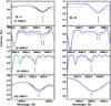 |
Fig. 1 Fits to the features C i 5380.3, C2 5635.2, CN 6332.2 and [OI] 6300.3 Å lines and bandheads, with the abundances reported in Table A.1, for the stars BL-5 and B3-f8. For BL-5 calculations with ±0.1 (green for minus, magenta for plus) for C, N and O are shown. |
In Table A.1 the original C, N and O abundances from Lecureur et al. (2007), the preliminary revision reported in Barbuy et al. (2015) and the presently fully revised C, N and O abundances for the 56 sample red giants are given.
3.2. Uncertainties
We have adopted uncertainties in the atmospheric parameters of ±150 K for effective temperature, ±0.20 for surface gravity, ±0.10 in [Fe/H] and ±0.10 km s-1 for microturbulent velocity, as explained in Barbuy et al. (2013).
The errors in the abundance ratios [O/Fe] were computed by fitting the C i, C2, CN and [OI] 6300.311 Å lines with the modified atmospheric model. The reported error corresponds to the difference needed to return from the value with the modified model atmosphere to the adopted one. The error in the element abundance ratios, induced by a change of ΔTeff = + 150 K, Δlog g = + 0.2 and Δvt = 0.1 km s-1 are given. We also add the error induced by a variation in the carbon abundances of Δ [C/Fe] = ± 0.1 and computed the error of a metallicity variation of Δ [Fe/H] = −0.1; the effect of the latter on abundance ratios is negligible. These errors and their quadratic sums are given in Table 1 for the star BL-5, noting that the total error is overestimated because the stellar parameters are covariant.
Abundance uncertainties for star BL-5.
3.3. Comparison with literature oxygen abundances
In Table 2 we report the stellar parameters and oxygen abundances by Ryde et al. (2010), where some stars of the present sample were observed in the infrared. There is good agreement between the results from the two analyses for the same stars.
In Fig. 2 we show [O/Fe] vs. [Fe/H] in the metallicity range −1.5 < [Fe/H] < + 0.7, with the present results compared to literature results for the bulge (upper panel), and for thick disk stars (lower panel). The bulge samples are the bulge dwarfs by Bensby et al. (2013), giant stars from Alves-Brito et al. (2010) that were carried out in the optical for the same stars as in Meléndez et al. (2008), Cunha & Smith (2006), Ryde et al. (2010), Rich et al. (2012), Johnson et al. (2014), Rich & Origlia (2005) and Fulbright et al. (2006, 2007).
In the lower panel, the present oxygen abundances for 56 bulge giants are plotted together with thick disc stars analysed by Alves-Brito et al. (2010), Bensby et al. (2004) and Reddy et al. (2006).
In Table 3 we have gathered the solar oxygen and iron abundances used by these different authors, and have applied a correction to all of them, to be compatible with the value given by Steffen et al. (2015) of A(O) = 8.76 and A(Fe) = 7.50. The reasoning is that if a higher A(O) value is assumed for the Sun, a lower value for the star will be given, therefore the correction has to be added to the oxygen abundances reported by the authors.
In Table 3 we also include the A(O) and A(Fe) solar abundances according to Allende-Prieto et al. (2001), Asplund et al. (2009), Grevesse & Sauval (1998), Lodders (2009), Kurucz (1993), and Steffen et al. (2015).
The presently revised oxygen abundances in bulge stars are in very good agreement with those by Cunha & Smith (2006) and Ryde et al. (2010), who used H-band OH lines to derive the oxygen abundances, taking into account the molecular dissociative equilibrium, and simultaneously deriving the carbon and nitrogen abundances. It appears to us that this is the reason for the agreement, and the reliability of these results. Rich et al. (2012) and Rich & Origlia (2005) also used infrared lines, and should have taken into account the C and N abundances, but the C and N abundances are not reported, and consequently their method is not clear. Bensby et al. (2013, and references therein) derived abundances for microlensed bulge dwarfs. They used the permitted 7774–7 Å oxygen triplet lines, which are strongly subject to NLTE effects (Kiselman 2001; Steffen et al. 2015). The higher effective temperatures of turn-off dwarfs imply that there is no significant molecule formation, and in this case, it is the NLTE effects that cause a tendency to yield higher oxygen abundances.
Fulbright et al. (2006, 2007), Alves-Brito et al. (2010) and Johnson et al. (2014) used the reliable line of [OI]6300 Å, but without taking the C and N abundances into consideration.
For these reasons, it appears that the present results, together with those by Ryde et al. (2010) and Cunha & Smith (2006) are, in principle, the correct ones.
The abundance results for 264 RGB giants in three off-axis fields (l,b) = (−5.5,−7), (−4, −9) and (+8.5, +9) from Johnson et al. (2013) were not included as although these authors took into account the C and N abundances very carefully, there is no mention of verification of blending with telluric lines. From some of their very high values of [O/Fe] it seems that there was contamination in a number of stars. Besides, and maybe partly due to this effect, the results show a large spread, and for this reason they were not considered here. Their Si and Ca abundances also show some spread, probably due to their use of low resolution (R ~ 18 000) spectra. On the other hand, their work provides important confirmation of similar mean [O/Fe], [Si/Fe], [Ca/Fe] vs. [Fe/H] in different locations in the bulge.
4. Chemical evolution models compared with alpha-element abundances
Oxygen: Figs. 3 and 4 compare the [O/Fe] vs. [Fe/H] data from the presently rederived oxygen abundances, and literature data for bulge giants from Cunha & Smith (2006) and Ryde et al. (2010), which we selected as being the most reliable results, to the predictions of the chemodynamical models for a classical bulge. Figures 3a and b, exhibits the results of the model with specific star-formation rates of νSF = 3 Gyr-1, with and without hypernovae. In the metallicity range considered, the effect of hypernovae is negligible, as can be verified in Fig. 3.
The comparison between the predictions of the models including hypernovae with those without them, shows that the nucleosynthesis prescriptions are not critical for the [O/Fe] ratios. In other words, the trend of [O/Fe] vs. [Fe/H] is a very robust indicator on the process of bulge formation. For this reason, despite the difficulties in obtaining oxygen abundances in bulge stars (for example due to NLTE effects on the permitted lines, or the need to take into account the carbon abundance when using the forbidden [OI]6300.3 Å line in cool stars), this effort is valuable because they are a prime probe for bulge formation.
Figures 4a and b shows the model predictions for νSF = 1 Gyr-1 and νSF = 0.5 Gyr-1. It appears that the specific star-formation rate in the range νSF = 0.5−1 Gyr-1 is appropriate for describing the oxygen abundances from the present work, together with the oxygen abundances from Cunha & Smith (2006) and Ryde et al. (2010). Figure 4c shows the same model as in panel a, but with a top-heavy IMF (xIMF = 1.05). This fit shows that a top-heavy IMF is not suitable.
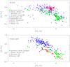 |
Fig. 2 [O/Fe] vs. [Fe/H] for present results compared with published abundances for halo and bulge stars. Panel a): plotted in the metallicity range −1.5 < [Fe/H] < + 0.7, corresponding to that of sample bulge giant stars, compared with the bulge dwarfs by Bensby et al. (2013), giant stars from Alves-Brito et al. (2010) which is a revision of Meléndez et al. (2008), Cunha & Smith (2006), Johnson et al. (2014), Rich & Origlia (2005) and Fulbright et al. (2006, 2007); panel b): bulge giants from the present work, and thick disk stars by Alves-Brito et al. (2010), Bensby et al. (2004) and Reddy et al. (2006). |
Oxygen in bulge vs. thick disk stars: Fig. 3c compares the same model as in panel a with the data for the thick disk dwarfs from Bensby et al. (2004) and thick disk giants from Alves-Brito et al. (2010), together with the present oxygen abundances for 56 bulge giants. It should be noted that a thick disk is formed by a series of processes that are not included in the present models. This comparison is intended to verify published conclusions on the bulge and thick disk stars which give the same results (Meléndez et al. 2008; Alves-Brito et al. 2010; Gonzalez et al. 2011), among others. In all cases the oxygen indicator is the forbidden [OI]6300 Å line. The data are overplotted with the present chemo-dynamical models as in Fig. 3a. In the metallicity range of thick disk stars (1.2 ≲ [Fe/H] ≲ 0.0) there is very good agreement between the present results on oxygen abundances for the bulge giants and thick disk stars by Bensby et al. (2004). Whereas the oxygen abundances from Bensby et al. (2004) are remarkably similar to the present bulge giants, the bulge thick disk giants by Alves-Brito et al. (2010) show higher abundances and do not fit the present results for bulge giants. Note that Alves-Brito et al. did not take into account the C and N abundances, and their results may be overestimates. The same is true for oxygen abundances in thick disk stars by Reddy et al. (2006), where the permitted OI 7774-7 Å lines were analysed.
A. Oxygen solar abundances from the literature.
A further inspection of published available data is given in Fig. 5, showing [O/Fe] vs. [Fe/H] for the present results for bulge giants compared to thick disk and bulge giants by Alves-Brito et al. (2010), and thick disk and bulge dwarfs by Bensby et al. (2004, 2013).
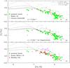 |
Fig. 3 [O/Fe] vs. [Fe/H] for the present results together with literature abundances for and bulge and thick disk stars and the predictions of the chemodynamical model for the bulge. Panel a): the data derived for the sample bulge giant stars are compared with the results for bulge giants from Cunha & Smith (2006) and Ryde et al. (2010). The lines are the predictions of the model assumig a specific star formation rate of νSF = 3 Gyr-1. Panel b): same data as in panel a) and the predicted O/Fe] vs. [Fe/H] for the model with no hypernovae. The dot-dashed line is the prediction by the model with hypernovae for r< 0.5 kpc; panel c): the [O/Fe] vs. [Fe/H] of the thick disk dwarfs from Bensby et al. (2004), thick disk giants from Alves-Brito et al. (2010) are superposed on the model predictions of panel a). |
We preferred to use only the sample and results from Bensby et al. (2004) for 73 dwarf F and G thick disk stars where the more reliable forbidden [OI] 6300.3 Å line was employed and did not use the Bensby et al. (2014) data for thick disk stars given the dispersion in the oxygen abundance.
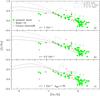 |
Fig. 4 [O/Fe] vs. [Fe/H] for the present results together with the results for bulge giants from Cunha & Smith (2006) and Ryde et al. (2010) are compared to the predictions of the chemodynamical model for the bulge. Panel a): results from the model with νSF = 1 Gyr-1. Panel b): results from the model with νSF = 0.5 Gyr-1. Panel c): the same model as in panel a), but with a top-heavy IMF (xIMF = 1.05). |
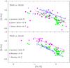 |
Fig. 5 [O/Fe] vs. [Fe/H]: present results for bulge giants compared to: a) thick disk and bulge giants. The lines are the linear regressions to the data with [Fe/H] ≥ −1.0; the upper blue line is the linear regression to the thick disk data and the lower magenta line is the linear regression to the bulge data. by Alves-Brito et al. (2010); b) thick disk and bulge dwarfs by Bensby et al. (2004, 2013). The upper magenta line is the linear regression to the bulge data and the lower blue line is the linear regression to the thick disk data. |
The present bulge giants and the bulge giants from Alves-Brito et al. (2010) show very good agreement. Despite the claim by Alves-Brito et al. (2010) that their bulge and thick disk giants show similar behaviour, a covariance analysis comparing the linear regressions of the two groups indicates that the thick disk giants have oxygen abundances higher than those of the bulge giants. A t-test applied to their data with [Fe/H] ≥ −1.0 allows for rejection of the null hypothesis that both subsamples are drawn from the same-population at a 0.03% significance level, providing an upward average shift of 0.20 for the [O/Fe] values of thick disk data with respect to the bulge data. Furthermore, the present bulge giants and the thick disk dwarfs by Bensby et al. (2004) show excellent agreement. Nevertheless, the bulge dwarfs by Bensby et al. (2013) are clearly enhanced with respect to the present bulge giants and thick disk dwarfs of Bensby et al. (2004). In this case, the covariance analysis rejects the hypothesis that both subsamples are drawn from the same-population at a <0.01% significance level, but providing a downward average shift of 0.30 for the [O/Fe] values of thick disk data with respect to the bulge data. These results illustrate why this discussion is inconclusive: it is not clear if the thick disk would be more oxygen-rich than bulge stars as hinted by results from Alves-Brito et al. (2010), or if the bulge stars would be more oxygen-rich than thick disk stars as can be seen from Bensby et al. (2004, 2013) data.
Recently, based on APOGEE data (Majewski et al. 2016), bulge giants were found to be more Mg-rich than thick disk stars by Schultheis et al. (2017), relaunching the discussion as to whether the bulge formation timescale has been faster than that of the thick disk.
Magnesium: Figs. 6 and 7 show published magnesium abundances from Gonzalez et al. (2011), Johnson et al. (2014) and Alves-Brito et al. (2010) that revise the same stars as in Meléndez et al. (2008) and Ryde et al. (2016) for red giants, from Hill et al. (2011) and Gonzalez et al. (2015) for Red Clump (RC) stars and from Bensby et al. (2013) for microlensed dwarfs. The data are compared with models with νSF = 3, 1 and 0.5 Gyr-1.
In Figs. 6a and 7a,b, the models fit the Hill et al. (2011) data well, but underestimate the other published results.
Similarly to oxygen, magnesium is mainly produced during the hydrostatic nuclear burning phases of SNII progenitors (WW95; Kobayashi et al. 2006). However, even for the case of an archetypical α element such as magnesium, the nucleosynthesis prescription should take into account the incompleteness of the reaction network and uncertainties in the nuclear physics and the locus where the element is produced. In particular, Woosley and Weaver (1995) models underestimate the [25Mg/24Mg] and [26Mg/24Mg] ratios at low metallicities (Timmes et al. 1995) and in addition, most of the 24Mg is not produced by the sequence of addition of α particles to 12C, 16O-20Ne-Mg24, but by direct carbon burning. Therefore, it is not recommended that other model parameters such as the IMF index be deduced from the Mg level of abundances. The underestimation of Mg yields by WW95 was already discussed by Argast et al. (2002), as being due to uncertainties in progenitor models prior to core-collapse, the crucial reaction rate 12C(α, γ)16O, convection treatment and explosion mechanisms and energies. The uncertainties on these processes can been narrowed by new nuclear data and ab initio calculations. Accordingly, since WW95, there have been updates in the nucleosynthesis models of massive stars (Kobayashi et al. 2006; Nomoto et al. 2013; West et al. 2016). Recently, Sukhbold et al. (2016) presented yields with models where the explosion energies were predicted rather than assumed. According to the authors, the yields on Mg and Al are still slightly deficient, possibly due to a low CO core-size, which in turn may be a consequence of neglecting rotation or differences in overshooting mixing.
In Fig. 6b, the [O/Mg] ratio, as extensively discussed by McWilliam (2016), shows a drop in [O/Mg] for super-metal-rich stars, which is not expected and could be due to selective winds in massive stars, as proposed by McWilliam (2016, and references therein), and regarded as a possibility by Kobayashi & Nakasato (2011), with the other possibility being some process that would change the C/O ratio. The present models include metallicity-dependent yields from stellar winds but do not discriminate among different elements.
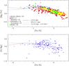 |
Fig. 6 [Mg/Fe] vs. [Fe/H] and [O/Mg] vs. [Fe/H] data from the literature for thick disk and bulge stars are compared to the predictions of the model with a specific star-formation rate of νSF = 3 Gyr-1. The references for the data points are: Alves-Brito et al. (2010), Hill et al. (2011), Bensby et al. (2013), Johnson et al. (2014), Gonzalez et al. (2015) and Ryde et al. (2016). |
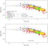 |
Fig. 7 [Mg/Fe] vs. [Fe/H] data from literature for thick disk and bulge stars are compared to the predicted [Mg/Fe] vs. [Fe/H] of the models with νSF = 1 Gyr-1 and νSF = 0.5 Gyr-1 using the references as in Fig. 6. |
Silicon, calcium, and titanium: Figs. 8–10 show the Si, Ca and Ti abundances in red giants published by Alves-Brito et al. (2010), Gonzalez et al. (2011), Johnson et al. (2014), and Ryde et al. (2016), in the Red Clump (RC) stars published by Gonzalez et al. (2015), and in microlensed dwarfs published by Bensby et al. (2013). These figures show that the chemo-dynamical models for νSF = 0.5 Gyr-1 fit the shape and location of the turnover, due to Fe enrichment by SNIa, for Si, and Ca, remarkably well. The level of abundances is better reproduced with νSF = 3 Gyr-1, but our results are sensitive to details of prescriptions. For Ti there could be a small shift between the models and the observations for the moderate metallicity interval −1.0 < [Fe/H] < −0.4. As pointed out by Timmes et al. (1995), Ti is underproduced in their models by at least a factor of two. Following this remark by Timmes et al. (1995), in our models we used yields for the Ti that are double those given in WW95. Even applying this correction, however, Ti abundances are still somewhat underpredicted, as noted above.
An important conclusion is that the SNIa enrichment, indicated by the knee where the [Si,Ca/Fe] ratios start to drop, located at [Fe/H] ~ −0.6–0.7, is suitably well-defined by the models.
A further important conclusion, reached by Johnson et al. (2013), Ryde et al. (2016) and McWilliam (2016), is that these alpha-elements show the same behaviour in all different parts of the Galactic bulge so far studied.
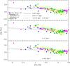 |
Fig. 8 [Si/Fe] vs. [Fe/H] data from the literature for halo and bulge stars are compared to the predictions of models with νSF = 3, 1 and 0.5 Gyr-1 using the same references as in Fig. 6. |
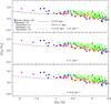 |
Fig. 9 [Ca/Fe] vs. [Fe/H] data from the literature for halo and bulge stars are compared to the predictions of models with νSF = 3, 1 and 0.5 Gyr-1 using the same references as in Fig. 6. |
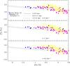 |
Fig. 10 [Ti/Fe] vs. [Fe/H] data from literature for halo and bulge stars are compared to the predictions of models with νSF = 3, 1 and 0.5 Gyr-1 using the same references as in Fig. 6. |
5. Conclusions
The present chemical evolution models describe a classical bulge, and they are robust enough to drive conclusions on the timescales for bulge formation as well as on chemical enrichment at moderately low metallicities. The following conclusions are drawn from the comparison of models with data:
-
a)
The model predictions including hypernovae as compared with those without them, indicate that the nucleosynthesis prescriptions are not critical for the [O/Fe] ratios. In other words, the trend of [O/Fe] vs. [Fe/H] is a very robust indicator of the process of bulge formation. It also applies to the other alpha-elements, however their nucleosynthetic production is more complex and includes contributions from SNIa for Ca and Ti. In general, the inclusion of hypernovae is only important for [Fe/H] < −2.0.
-
b)
Another result from the models that is confirmed by the data is the [alpha/Fe] ~ + 0.25 ± 0.5 values at the solar metallicity [Fe/H] = 0.0 for Si, Ca and Ti. The [Si,Ca/Fe] ~ + 0.25 and [Ti/Fe] ~ + 0.10 at [Fe/H] = 0.0 is a consequence of a fast SFR in the bulge. For Mg, a high value only corresponds to the innermost bulge regions in the models. There is a spread in the data, and the Mg abundances by Hill et al. (2011) that appear reliable include stars with [Mg/Fe] ~ 0.0 at [Fe/H] = 0.0, and these are well matched by the model predictions for the 0.5 <r(kpc) < 1 region. However, as mentioned before, the nucleosynthesis prescriptions for Mg could be underestimates, as remarked by Timmes et al. (1995). For oxygen instead, [O/Fe] is close to the solar value at [Fe/H] = 0.0, which would imply a decrease in oxygen enrichment with increasing metallicity, as already pointed out by McWilliam et al. (2008) and McWilliam (2016).
-
c)
The spread in the data is partially due to observational uncertainties, but on the other hand, a true spread is expected from the location of star formation, as can be seen in Figs. 3 and 4, where the model predictions are shown for shells at different distances from the Galactic centre. The intrinsic spread in the [O/Fe] values reflects a spread in the radial distance at which star formation occurs.
- d)
As regards the IMF, as stated in Sect. 2, our adopted IMF assumes the usual Salpeter index xIMF = 1.35 and extends to 100 M⊙, whereas some chemical evolution models by other authors assume a different IMF. The possibility that the high mass cutoff could be smaller than the value of 100 M⊙, as explored by Tsujimoto et al. (1995), seems to be excluded by the statistics of gravitational wave sources, and in particular by the event GW150914 due to the merger of two ~30 M⊙ black holes (Abbott et al. 2016). High-mass black holes shoud not be very rare, which implies that the IMF extends up to at least 100 M⊙ and probably up to 150 M⊙ (Belczynski et al. 2016), and even up to 300 M⊙ (Eldridge & Stanway 2016). On the other hand, we tested the hypothesis of a top-heavy IMF (Tsujimoto & Bekki 2012), by adopting their choice xIMF = 1.05 for the model shown in Fig. 4. It is clear that such models give oxygen abundances at all metallicities that are too high.
- e)
An important indicator of chemical enrichment suitability is the start of contributions by SNe Ia that appear as a turnover in the [α/Fe] ratio, corresponding to the enrichment of Fe by SNe Ia. The turnover point for the thick disk stars is seen at −0.8 < [Fe/H] < −0.7 in data points by Reddy et al. (2006), at −0.7 < [Fe/H] < −0.6 in Alves-Brito et al. (2010), and at [Fe/H] ~ −0.6 in Bensby et al. (2004; see Fig. 3c). For the bulge stars, the metallicity at which the turnover occurs is less clear from the data, given the spread in abundances: according to the present results, from oxygen (Figs. 2–4) it is approximately −0.6 < [Fe/H] < −0.7, but there are not enough stars around these metallicities; it seems to be at [Fe/H] ~ −0.3 from data provided by Johnson et al. (2014) and at −0.6 < [Fe/H] < −0.5 from that provided by Bensby et al. (2013) and Ryde et al. (2010). The data on [Mg/Fe] (Fig. 6a) indicate a knee at approximately −0.8 < [Fe/H] < −0.6. We note that the ratio [Mg/O] should not be affected by yields from SNe Ia (Fig. 6b). [Si/Fe] and [Ca/Fe] in Figs. 8 and 9 show a turnover at −0.8 < [Fe/H] < −0.6. In the case of the [Si/Fe] and [Ca/Fe] trends with metallicity, the decrease is flatter in the range −0.6 < [Fe/H] < −0.2 relative to [Mg/Fe]. As regards Ti, there is no evidence of a knee from either models or observations (see Fig. 10).
- f)
The turnover is related to the question of how fast the bulge chemical enrichment was. The models for νSF = 0.5 to 1.0 Gyr-1 appear to be more suitable for producing the decrease in oxygen abundances at the higher metallicities, and also the oxygen abundances at the lower metallicities. The two data points at [Fe/H] ~ −1.2 would indicate the slower star-formation timescale of 2 Gyr. On the other hand, the present models with 0.3 Gyr-1 reproduce the higher oxygen abundances by Bensby et al. (2013) and Johnson et al. (2014) well. If the lower abundance points are correct, as we claim, they could provide information on (i) the nucleosynthetic process in low metallicity high-mass-type SNe II; (ii) the upper mass limit in the IMF (e.g. Tsujimoto et al. (1995) and (iii) the timescales of bulge formation. The general trends of Si and Ca abundance ratios vs. [Fe/H] are better fitted for 3 Gyr-1 in terms of absolute abundances, whereas 0.5 Gyr-1 better reproduces the turnover in Si and Ca. For Ti, the level of abundances tends to be lower in the models relative to the data. According to Timmes et al. (1995), their models underpredict the Ti abundances over all metallicities. Therefore, the level of Si, Ca and Ti abundances could be used to refine the nucleosynthesis prescriptions adopted in the model, in addition to being interpreted in terms of history of bulge formation. These elements result from both hydrostatic and explosive nucleosynthesis, which makes their predictions more complex than for O and Mg that are produced in hydrostatic phases only. Kobayashi & Nakasato (2011) presented a chemodynamical model for the Milky Way Galaxy. Their bulge component seems to be larger than the Galactic bulge, and should correspond better to the M31 bulge; in general, their calculations are applicable to the Galactic bulge. In Kobayashi & Nakasato (2011; their Fig. 17), there is a transition at [Fe/H] ~ −0.1 to +0.3 that corresponds to a fast SFR. In their model, an initial starburst is induced by the assembling of proto-clumps, when most stars are formed in the first 2 Gyr. Similarly, Nakasato & Nomoto (2003), using a smoothed particle hydrodynamics (SPH) code for the evolution of the Galaxy with star-formation processes, found that a spheroidal bulge is formed early, and a bar is formed afterwards. They propose that the bulge has two components, an early sub-galactic clump merger in the proto-Galaxy, and the bar that has formed gradually in the inner disk. At the stage of bulge formation from early mergers, 60% of bulge stars are formed in 0.5 Gyr. The turnover occurs at [Fe/H] ~ 0. The models by Cescutti & Matteucci (2011), show a turnover at [Fe/H] ~ + 0.3, due to a very fast timescale of νSF ~ 10 Gyr-1. A turnover at high metallicities of [Fe/H] ~ 0.0 is not confirmed by the data, and we suggest that the longer bulge formation timescales are more suitable.
-
g)
A comparison with models including the formation of a bar was also carried out. Cavichia et al. (2014) models consider a bulge formed in a collapse timescale of 2 Gyr, or νSF = 0.5 Gyr-1. The inclusion of radial inflow of gas, through the bar, does not affect the bulge metallicity distribution function (MDF), given that the bulk of bulge stars formed in a much shorter timescale before bar formation. The bulge collapse timescale of 1–2 Gyr of Cavichia et al. (2014), similarly to our models with νSF = 1−0.5 Gyr-1, better explain the data points with higher metallicity and lower [O/Fe] ratios (Fig. 4). For Mg, the νSF = 0.5 Gyr-1 fits the Mg data by Hill et al. (2011) very well, whereas even our higher νSF = 3 Gyr-1 (fastest timescale) cannot fit the other literature data. McWilliam (2016) discusses the difficulties in deriving reliable Mg abundances.
Tsujimoto & Bekki (2012) produce a fast formation of a metal-poor population in the bulge and thick disk, reaching ([Fe/H], [Mg/H], [Ba/H] ) = (−1.3, −0.9, −1.1); the metal-rich population forms subsequently from remaining gas, plus inflow from the inner disk, when the bar also forms (after the metal-poor population was formed). According to Nakasato & Nomoto (2003), the bar forms after the bulge, therefore even if there is radial inflow of gas and stars into the bulge, this could be considered a late event in the evolution of a classical bulge. This two-stage formation history of the bulge is confirmed by the observations, given that the bulge shows the characteristics of a classical bulge and also that of a pseudo-bulge. Babusiaux (2010, 2014) has shown, from kinematics and metallicity data for a large sample of stars, that metal-poor stars are found in a spheroidal distribution, and metal-rich ones in a bar-like distribution.
Acknowledgments
We are very grateful for the extremely useful comments from the referee. A. C. S. F. and B. B. acknowledge partial financial support by CNPq, CAPES, and FAPESP.
References
- Abbott, B. P., Abbott, R., Abbott, T. D., et al. 2016, Phys. Rev. Lett., 116, 061102 [Google Scholar]
- Allen de Prieto, C., Lambert, D. L., & Asplund, M. 2001, ApJ, 556, L63 [NASA ADS] [CrossRef] [Google Scholar]
- Alves-Brito, A., Meléndez, J., Asplund, M., et al. 2010, A&A, 513, A35 [NASA ADS] [CrossRef] [EDP Sciences] [Google Scholar]
- Argast, D., Samland, M., Thielemann, F.-K., & Gerhard, O. E. 2002, A&A, 388, 842 [NASA ADS] [CrossRef] [EDP Sciences] [Google Scholar]
- Asplund, M., Grevesse, N., Sauval, A. J., & Scott, P. 2009, ARA&A, 47, 481 [NASA ADS] [CrossRef] [Google Scholar]
- Babusiaux, C., Gómez, A., Hill, V., et al. 2010, A&A, 519, A77 [NASA ADS] [CrossRef] [EDP Sciences] [Google Scholar]
- Babusiaux, C., Katz, D., Hill, V., et al. 2014, A&A, 563, A15 [NASA ADS] [CrossRef] [EDP Sciences] [Google Scholar]
- Ballero, S. K., Matteucci, F., Origlia, L., & Rich, R. M. 2007, A&A, 467, 123 [Google Scholar]
- Barbuy, B., Perrin, M.-N., Katz, D., et al. 2003, A&A, 404, 661 [NASA ADS] [CrossRef] [EDP Sciences] [Google Scholar]
- Barbuy, B., Hill, V., Zoccali, M., et al. 2013, A&A, 559, A5 [NASA ADS] [CrossRef] [EDP Sciences] [Google Scholar]
- Barbuy, B., Friaça, A., da Silveira, C. R., et al. 2015, A&A, 580, A40 [NASA ADS] [CrossRef] [EDP Sciences] [Google Scholar]
- Belczynski, K., Holz, D. E., Bulik, T., & O’Shaughnessy, R. 2016, Nature, 534, 512 [NASA ADS] [CrossRef] [Google Scholar]
- Bensby, T., Feltzing, S., & Lundström, I. 2004, A&A, 415, 155 [NASA ADS] [CrossRef] [EDP Sciences] [Google Scholar]
- Bensby, T., Yee, J. C., Feltzing, S., et al. 2013, A&A, 549, A147 [NASA ADS] [CrossRef] [EDP Sciences] [Google Scholar]
- Bensby, T., Feltzing, S., & Oey, M. S. 2014, A&A, 562, A71 [NASA ADS] [CrossRef] [EDP Sciences] [Google Scholar]
- Cardelli, J. A., Clayton, G. C., & Mathis, J. S. 1989, ApJ, 345, 245 [NASA ADS] [CrossRef] [Google Scholar]
- Cavichia, O., Mollá, M., Costa, R. D. D., & Maciel, W. J. 2014, MNRAS, 437, 3688 [NASA ADS] [CrossRef] [Google Scholar]
- Cescutti, G., & Matteucci, F. 2011, A&A, 525, A126 [NASA ADS] [CrossRef] [EDP Sciences] [Google Scholar]
- Coelho, P., Barbuy, B., Meléndez, J., et al. 2005, A&A, 443, 735 [NASA ADS] [CrossRef] [EDP Sciences] [Google Scholar]
- Cunha, K., & Smith, V. V. 2006, ApJ, 652, 491 [NASA ADS] [CrossRef] [Google Scholar]
- Davis, S. P., & Phillips, J. G. 1963, The Red System (A2Π-X2Σ) of the CN molecule (Berkeley: University of California Press) [Google Scholar]
- Dobrovolskas, V., Kucinskas, A., Bonifacio, P., et al. 2015, A&A, 576, A128 [NASA ADS] [CrossRef] [EDP Sciences] [Google Scholar]
- Eldridge, J. J., & Stanway, E. R. 2016, MNRAS, 462, 3302 [NASA ADS] [CrossRef] [Google Scholar]
- Friaça, A. C. S., & Terlevich, R. J. 1998, MNRAS, 298, 399 [NASA ADS] [CrossRef] [Google Scholar]
- Fröhlich, C., Hauser, P., Liebendörfer, M., et al. 2006, ApJ, 637, 415 [Google Scholar]
- Fulbright, J. P., McWilliam, A., & Rich, R. M. 2006, ApJ, 636, 821 [NASA ADS] [CrossRef] [Google Scholar]
- Fulbright, J. P., McWilliam, A., & Rich, R. M. 2007, ApJ, 661, 1152 [NASA ADS] [CrossRef] [Google Scholar]
- Gonzalez, O. A., Rejkuba, M., Zoccali, M., et al. 2011, A&A, 530, A54 [NASA ADS] [CrossRef] [EDP Sciences] [Google Scholar]
- Gonzalez, O. A., Zoccali, M., Vasquez, S., et al. 2015, A&A, 584, A46 [NASA ADS] [CrossRef] [EDP Sciences] [Google Scholar]
- Greggio, L., & Renzini, A. 1983, A&A, 118, 217 [NASA ADS] [Google Scholar]
- Grevesse, N., & Sauval, J. N. 1998, Space Sci. Rev., 35, 161 [NASA ADS] [CrossRef] [Google Scholar]
- Grieco, V., Matteucci, F., Pipino, A., & Cescutti, G. 2012, A&A, 548, A60 [NASA ADS] [CrossRef] [EDP Sciences] [Google Scholar]
- Gustafsson, B., Edvardsson, B., Eriksson, K., et al. 2008, A&A, 486, 951 [NASA ADS] [CrossRef] [EDP Sciences] [Google Scholar]
- Hill, V., Lecureur, A., Gómez, A., et al. 2011, A&A, 534, A80 [NASA ADS] [CrossRef] [EDP Sciences] [Google Scholar]
- Iwamoto, K., Brachwitz, F., Nomoto, K., et al. 1999, ApJS, 125, 439 [NASA ADS] [CrossRef] [MathSciNet] [Google Scholar]
- Johnson, C. I., Rich, R. M., Kobayashi, C., et al. 2013, ApJ, 765, 157 [NASA ADS] [CrossRef] [Google Scholar]
- Johnson, C. I., Rich, R. M., Kobayashi, C., et al. 2014, AJ, 148, 67 [NASA ADS] [CrossRef] [Google Scholar]
- Kiselman, D. 2001, New Astron. Rev., 45, 559 [NASA ADS] [CrossRef] [Google Scholar]
- Kobayashi, C., & Nakasato, N. 2011, ApJ, 729, 16 [NASA ADS] [CrossRef] [Google Scholar]
- Kobayashi, C., Umeda, H., Nomoto, K., et al. 2006, ApJ, 653, 1145 [NASA ADS] [CrossRef] [Google Scholar]
- Kurúcz, R. 1993, Kurucz CD-ROM No. 23 (Cambridge, Mass.: Smithsonian Astrophysical Observatory) [Google Scholar]
- Lecureur, A., Hill, V., Zoccali, M., Barbuy, B., et al. 2007, A&A, 465, 799 [NASA ADS] [CrossRef] [EDP Sciences] [Google Scholar]
- Lodders, K., Palme, H., Gail, H.-P. 2009, Landolt-Börnstein – Group VI Astronomy and Astrophysics Numerical Data and Functional Relationships in Science and Technology Volume 4B: Solar System, ed. J. E. Trümper, 4.4., 44 [Google Scholar]
- Majewski, S. R., Schiavon, R. P., Frinchaboy, P. M., et al. 2016, AJ, in press [arXiv:1509.05420] [Google Scholar]
- Matteucci, F. 1992, ApJ, 397, 32 [NASA ADS] [CrossRef] [Google Scholar]
- Matteucci, F., & Brocato, E. 1990, ApJ, 365, 539 [NASA ADS] [CrossRef] [Google Scholar]
- Matteucci, F., & Tornambè, A. 1987, A&A, 185, 51 [NASA ADS] [Google Scholar]
- McWilliam, A. 2016, PASA, 33, 40 [NASA ADS] [CrossRef] [Google Scholar]
- McWilliam, A., Matteucci, F., Ballero, S., et al. 2008, ApJ, 136, 367 [Google Scholar]
- Meléndez, J., Asplund, M., Alves-Brito, A., et al. 2008, A&A, 484, L21 [NASA ADS] [CrossRef] [EDP Sciences] [MathSciNet] [Google Scholar]
- Nakasato, N., & Nomoto, K. 2003, ApJ, 588, 842 [NASA ADS] [CrossRef] [Google Scholar]
- Nissen, P. E., Primas, F., Asplund, M., & Lambert, D. L. 2002, A&A, 390, 235 [NASA ADS] [CrossRef] [EDP Sciences] [Google Scholar]
- Nomoto, K., Tominaga, N., Umeda, H., Kobayashi, C., & Maeda, K. 2006, Nucl. Phys. A, 777, 424 [NASA ADS] [CrossRef] [Google Scholar]
- Nomoto, K., Kobayashi, C., & Tominaga, N. 2013, ARA&A, 51, 457 [NASA ADS] [CrossRef] [Google Scholar]
- Planck Collaboration I. 2016, A&A, 594, A1 [NASA ADS] [CrossRef] [EDP Sciences] [Google Scholar]
- Reddy, B. E., Lambert, D. L., & Allen de Prieto, C. 2006, MNRAS, 367, 1329 [NASA ADS] [CrossRef] [Google Scholar]
- Rich, R. M., & Origlia, L. 2005, ApJ, 634, 1293 [NASA ADS] [CrossRef] [MathSciNet] [Google Scholar]
- Rich, R. M., Origlia, L., & Valenti, E. 2012, ApJ, 746, 59 [NASA ADS] [CrossRef] [Google Scholar]
- Ryde, N., Gustafsson, B., Edvardsson, B., et al. 2010, A&A, 509, A20 [NASA ADS] [CrossRef] [EDP Sciences] [Google Scholar]
- Ryde, N., Schultheis, M., Grieco, V., et al. 2016, AJ, 151, 1 [NASA ADS] [CrossRef] [Google Scholar]
- Samland, M., & Gerhard, O. E. 2003, A&A, 399, 961 [NASA ADS] [CrossRef] [EDP Sciences] [Google Scholar]
- Schultheis, M., Rojas-Arriagada, A., García-Perez, A. E., et al. 2017, A&A, accepted [Google Scholar]
- Steffen, M., Prakapavicius, D., Caffau, E., et al. 2015, A&A, 583, A57 [NASA ADS] [CrossRef] [EDP Sciences] [Google Scholar]
- Sukhbold, T., Ertl, T., Woosley, S. E., et al. 2016, ApJ, 821, 38 [Google Scholar]
- Timmes, F. X., Woosley, S. E., & Weaver, T. A. 1995, ApJS, 98, 617 [NASA ADS] [CrossRef] [Google Scholar]
- Tsujimoto, T., & Bekki, K. 2012, ApJ, 747, 125 [NASA ADS] [CrossRef] [Google Scholar]
- Tsujimoto, T., Yoshii, Y., & Nomoto, K., Shigeyama, T. 1995, A&A, 302, 704 [NASA ADS] [Google Scholar]
- Umeda, H., & Nomoto, K. 2002, ApJ, 565, 385 [NASA ADS] [CrossRef] [Google Scholar]
- Umeda, H., & Nomoto, K. 2003, Nature, 422, 871 [NASA ADS] [CrossRef] [PubMed] [Google Scholar]
- Umeda, H., & Nomoto, K. 2005, ApJ, 619, 427 [NASA ADS] [CrossRef] [Google Scholar]
- West, C., Heger, A., & Austin, S. M. 2013, ApJ, 769, 2 [NASA ADS] [CrossRef] [Google Scholar]
- van de Hoek, L. B., & Groenewegen, M. A. T. 1997, A&A, 123, 305 [NASA ADS] [CrossRef] [EDP Sciences] [Google Scholar]
- Woosley, S. E., & Weaver, T. A. 1995, ApJS, 101, 181 [NASA ADS] [CrossRef] [Google Scholar]
- Wyse, R. F. G., & Gilmore, G. 1992, AJ, 104, 144 [NASA ADS] [CrossRef] [Google Scholar]
- Zoccali, M., Lecureur, A., Barbuy, B., et al. 2006, A&A, 457, L1 [NASA ADS] [CrossRef] [EDP Sciences] [Google Scholar]
- Zoccali, M., Hill, V., Lecureur, A., et al. 2008, A&A, 486, 177 [NASA ADS] [CrossRef] [EDP Sciences] [Google Scholar]
Appendix A: Re-derived C, N, and O abundances
All Tables
All Figures
|
Fig. 1 Fits to the features C i 5380.3, C2 5635.2, CN 6332.2 and [OI] 6300.3 Å lines and bandheads, with the abundances reported in Table A.1, for the stars BL-5 and B3-f8. For BL-5 calculations with ±0.1 (green for minus, magenta for plus) for C, N and O are shown. |
| In the text | |
|
Fig. 2 [O/Fe] vs. [Fe/H] for present results compared with published abundances for halo and bulge stars. Panel a): plotted in the metallicity range −1.5 < [Fe/H] < + 0.7, corresponding to that of sample bulge giant stars, compared with the bulge dwarfs by Bensby et al. (2013), giant stars from Alves-Brito et al. (2010) which is a revision of Meléndez et al. (2008), Cunha & Smith (2006), Johnson et al. (2014), Rich & Origlia (2005) and Fulbright et al. (2006, 2007); panel b): bulge giants from the present work, and thick disk stars by Alves-Brito et al. (2010), Bensby et al. (2004) and Reddy et al. (2006). |
| In the text | |
|
Fig. 3 [O/Fe] vs. [Fe/H] for the present results together with literature abundances for and bulge and thick disk stars and the predictions of the chemodynamical model for the bulge. Panel a): the data derived for the sample bulge giant stars are compared with the results for bulge giants from Cunha & Smith (2006) and Ryde et al. (2010). The lines are the predictions of the model assumig a specific star formation rate of νSF = 3 Gyr-1. Panel b): same data as in panel a) and the predicted O/Fe] vs. [Fe/H] for the model with no hypernovae. The dot-dashed line is the prediction by the model with hypernovae for r< 0.5 kpc; panel c): the [O/Fe] vs. [Fe/H] of the thick disk dwarfs from Bensby et al. (2004), thick disk giants from Alves-Brito et al. (2010) are superposed on the model predictions of panel a). |
| In the text | |
|
Fig. 4 [O/Fe] vs. [Fe/H] for the present results together with the results for bulge giants from Cunha & Smith (2006) and Ryde et al. (2010) are compared to the predictions of the chemodynamical model for the bulge. Panel a): results from the model with νSF = 1 Gyr-1. Panel b): results from the model with νSF = 0.5 Gyr-1. Panel c): the same model as in panel a), but with a top-heavy IMF (xIMF = 1.05). |
| In the text | |
|
Fig. 5 [O/Fe] vs. [Fe/H]: present results for bulge giants compared to: a) thick disk and bulge giants. The lines are the linear regressions to the data with [Fe/H] ≥ −1.0; the upper blue line is the linear regression to the thick disk data and the lower magenta line is the linear regression to the bulge data. by Alves-Brito et al. (2010); b) thick disk and bulge dwarfs by Bensby et al. (2004, 2013). The upper magenta line is the linear regression to the bulge data and the lower blue line is the linear regression to the thick disk data. |
| In the text | |
|
Fig. 6 [Mg/Fe] vs. [Fe/H] and [O/Mg] vs. [Fe/H] data from the literature for thick disk and bulge stars are compared to the predictions of the model with a specific star-formation rate of νSF = 3 Gyr-1. The references for the data points are: Alves-Brito et al. (2010), Hill et al. (2011), Bensby et al. (2013), Johnson et al. (2014), Gonzalez et al. (2015) and Ryde et al. (2016). |
| In the text | |
|
Fig. 7 [Mg/Fe] vs. [Fe/H] data from literature for thick disk and bulge stars are compared to the predicted [Mg/Fe] vs. [Fe/H] of the models with νSF = 1 Gyr-1 and νSF = 0.5 Gyr-1 using the references as in Fig. 6. |
| In the text | |
|
Fig. 8 [Si/Fe] vs. [Fe/H] data from the literature for halo and bulge stars are compared to the predictions of models with νSF = 3, 1 and 0.5 Gyr-1 using the same references as in Fig. 6. |
| In the text | |
|
Fig. 9 [Ca/Fe] vs. [Fe/H] data from the literature for halo and bulge stars are compared to the predictions of models with νSF = 3, 1 and 0.5 Gyr-1 using the same references as in Fig. 6. |
| In the text | |
|
Fig. 10 [Ti/Fe] vs. [Fe/H] data from literature for halo and bulge stars are compared to the predictions of models with νSF = 3, 1 and 0.5 Gyr-1 using the same references as in Fig. 6. |
| In the text | |
Current usage metrics show cumulative count of Article Views (full-text article views including HTML views, PDF and ePub downloads, according to the available data) and Abstracts Views on Vision4Press platform.
Data correspond to usage on the plateform after 2015. The current usage metrics is available 48-96 hours after online publication and is updated daily on week days.
Initial download of the metrics may take a while.