| Issue |
A&A
Volume 598, February 2017
|
|
|---|---|---|
| Article Number | A13 | |
| Number of page(s) | 13 | |
| Section | Stellar structure and evolution | |
| DOI | https://doi.org/10.1051/0004-6361/201629112 | |
| Published online | 24 January 2017 | |
Non-thermal radiation from a pulsar wind interacting with an inhomogeneous stellar wind
1 Departament d’Astronomia i MeteorologiaInstitut de Ciènces del Cosmos, Universitat de Barcelona, IEEC-UB, Martí i Franquès 1, 08028 Barcelona, Spain
e-mail: vmdelacita@am.ub.es
2 Department of Physics, Rikkyo University 3-34-1, Nishi-Ikebukuro, Toshima-ku, 171-8501 Tokyo, Japan
3 Departament d’Astronomia i Astrofísica, Universitat de València, Av. Vicent Andrés Estellés s/n, 46100 Burjassot (València), Spain
4 Observatori Astronòmic, Universitat de València, C/ Catedràtic José Beltran, 2, 46980 Paterna (València), Spain
Received: 14 June 2016
Accepted: 11 November 2016
Context. Binaries hosting a massive star and a non-accreting pulsar are powerful non-thermal emitters owing to the interaction of the pulsar and the stellar wind. The winds of massive stars are thought to be inhomogeneous, which could have an impact on the non-thermal emission.
Aims. We study numerically the impact of the presence of inhomogeneities or clumps in the stellar wind on the high-energy non-thermal radiation of high-mass binaries hosting a non-accreting pulsar.
Methods. We compute the trajectories and physical properties of the streamlines in the shocked pulsar wind without clumps, with a small clump, and with a large clump. This information is used to characterize the injection and the steady state distribution of non-thermal particles accelerated at shocks formed in the pulsar wind. The synchrotron and inverse Compton emission from these non-thermal particles is calculated, accounting also for the effect of gamma-ray absorption through pair creation. A specific study is done for PSR B1259-63/LS2883.
Results. When stellar wind clumps perturb the two-wind interaction region, the associated non-thermal radiation in the X-ray band, of synchrotron origin, and in the GeV–TeV band, of inverse Compton origin, is affected by several equally important effects: (i) strong changes in the plasma velocity direction that result in Doppler boosting factor variations; (ii) strengthening of the magnetic field that mainly enhances the synchrotron radiation; (iii) strengthening of the pulsar wind kinetic energy dissipation at the shock, potentially available for particle acceleration; and (iv) changes in the rate of adiabatic losses that affect the lower energy part of the non-thermal particle population. The radiation above 100 GeV detected, presumably, during the post-periastron crossing of the Be star disc in PSR B1259-63/LS2883, can be roughly reproduced assuming that the crossing of the disc is modelled as the encounter with a large inhomogeneity.
Conclusions. Because of the likely diverse nature of clumps in the stellar wind, and hydrodynamical instabilities, the non-thermal radiation of high-mass binaries with a non-accreting pulsar is expected to be boosted somewhat chaotically, and to present different superimposed variability patterns. Some of the observed variability in gamma rays from PSR B1259-63/LS2883 is qualitatively reproduced by our calculations.
Key words: hydrodynamics / pulsars: general / radiation mechanisms: non-thermal / stars: winds, outflows / stars: massive
© ESO, 2017
1. Introduction
In binaries hosting a high-mass star and a young non-accreting pulsar, strong interaction between the relativistic pulsar wind and the stellar wind is expected. In these wind collisions, efficient particle acceleration and non-thermal emission can take place (Maraschi & Treves 1981; Tavani et al. 1994), which would be behind the emission observed from radio to gamma rays in some of these objects, like PSR B1259-63/LS2883 (e.g. Aharonian et al. 2005; Chernyakova et al. 2014). Given that this emission, or at least a significant fraction of it, is expected to originate in the region where the winds collide, a proper characterization of the stellar and the pulsar wind is needed to understand the involved physical processes.
Density inhomogeneities, or clumps, are thought to be present in the stellar winds of early-type stars (Lucy & Solomon 1970). The hydrodynamical and radiative consequences of the presence of clumps were studied analytically in Bosch-Ramon (2013), and relativistic, axisymmetric, hydrodynamical (RHD) simulations were carried out by Paredes-Fortuny et al. (2015) to study in more detail the impact of different types of clumps on the two-wind interaction region. It was found that clumps can noticeably affect the shape, size, and the stability of the interaction structure, and the variability patterns of the radiation coming from the structure. It was also proposed that wind inhomogeneities could be responsible of the GeV flare in PSR B1259-63/LS2883 (Chernyakova et al. 2014), and may also play an important role in the X-ray activity of some binaries (see e.g. the discussion in Bosch-Ramon 2013, and references therein). However, the impact of the presence of inhomogeneities in the stellar wind in the high-energy emission has not been accurately studied yet.
In this work, we compute for the first time the synchrotron and IC emission produced by the interaction of an inhomogeneous1 stellar wind and a pulsar wind based on hydrodynamic simulations, obtaining the spectral energy distributions (SED) and maps of the emitting region. To characterize the impact of wind inhomogeneities on the non-thermal radiation, we have used the flow information obtained from the RHD simulations done by Paredes-Fortuny et al. (2015). From the flow hydrodynamical quantities, we have obtained a number of streamlines, characterizing the fluid of interest in the form of several 1D structures from which, following the method described in de la Cita et al. (2016), we compute the synchrotron and the inverse Compton (IC) radiation. As the stellar photon field is very dense, gamma-ray absorption due to electron-positron pair creation has been taken into account. An approach similar to the one adopted here was followed by Dubus et al. (2015) in a broad study of the non-thermal emission of high-mass binaries hosting a non-accreting pulsar, although in that case the stellar wind was assumed to be homogeneous.
A region of a size similar to the star-pulsar separation distance is considered. The reasons are threefold: (i) in this paper, we are mostly concerned with the main radiation features resulting from the interaction of a clump with the two-wind collision structure; (ii) we are interested in the highest energies, which are expected to be produced on the binary scales (however, see Zabalza et al. 2013); (iii) for reasons explained in Paredes-Fortuny et al. (2015), simulation results were limited to these scales. Since radio emission is expected to be produced far from the binary system (e.g. Dubus 2006b; Bosch-Ramon 2011), the focus here is put on X-rays and gamma rays.
Regarding the most recent simulations of stellar and pulsar winds collisions, few important differences from our work are to be mentioned. The simulations in Dubus et al. (2015) are three-dimensional (3D), whereas here the hydrodynamical results are taken from the simulations of Paredes-Fortuny et al. (2015), carried out with axisymmetry (2D). In addition, the grid was significantly larger in Dubus et al. (2015) than in Paredes-Fortuny et al. (2015). Regarding Bosch-Ramon et al. (2015), the 3D simulations included orbital motion, which proved to be important beyond few star-pulsar separation distances. That said, we note that the relatively small size of the computational grid in the present work allows orbital motion to be neglected, although instability development may be slower in our 2D simulations (see Sect. 2), and 3D calculations may yield remarkable quantitative differences in general. We note as well that the dynamical role of the magnetic field was not included in Paredes-Fortuny et al. (2015). So far, only Bogovalov et al. (2012) have included the magnetic field when computing the two-wind interaction structure in the context of binary systems, whereas several works have studied the magnetohydrodynamics in 1D, 2D and 3D, and in some cases the radiation for isolated pulsars interacting with the environment in the relativistic regime (e.g. Bucciantini et al. 2005; Volpi et al. 2008; Olmi et al. 2014; Porth et al. 2014; Morlino et al. 2015; Yoon & Heinz 2017, and references therein).
The paper is organized as follows: in Sect. 2 we describe the hydrodynamic set-up and results; in Sect. 3 we present the radiative computation results for the different cases of study together with an application to the gamma-ray binary PSR B1259-63/LS2883; finally, in Sects. 4 and 5 we sum up our conclusions and discuss the results.
2. Hydrodynamics
In this section, we summarize the numerical simulations from which the hydrodynamical information is obtained. In addition, we also briefly explain how the pulsar wind is characterized as a set of streamlines. For further details on the hydrodynamical simulations and on the mathematical procedure to obtain the streamlines, we refer to Paredes-Fortuny et al. (2015) and de la Cita et al. (2016; Appendix A), respectively. The code used in these simulations is a finite-volume, high-resolution shock-capturing scheme that solves the equations of relativistic hydrodynamics in conservation form. This code is an upgrade of that described in Martí et al. (1997), parallelized using OMP directives (Perucho et al. 2005). The numerical fluxes at cell boundaries are computed using an approximate Riemann solver that uses the complete characteristic information contained in the Riemann problems between adjacent cells (Donat & Marquina 1996). It is based on the spectral decomposition of the Jacobian matrices of the relativistic system of equations derived in Font et al. (1994), and uses analytical expressions for the left eigenvectors (Donat et al. 1998). The spatial accuracy of the algorithm is improved up to third order by means of a conservative monotonic parabolic reconstruction of the pressure, proper rest-mass density and the spatial components of the fluid four-velocity (PPM, see Colella & Woodward 1984; and Martí & Müller 2015). Integration in time is done simultaneously in both spatial directions using a multi-step total-variation-diminishing (TVD) Runge-Kutta (RK) method developed by Shu & Osher (1988), which provides third order in time. The simulations were run in a workstation with two Intel(R) Xeon(R) CPU E5-2643 processors (3.30 GHz, 4 × 2 cores, with two threads for each core) and four modules of 4096 MB of memory (DDR3 at 1600 MHz).
Paredes-Fortuny et al. (2015) performed axisymmetric RHD simulations of the interaction of a relativistic pulsar wind and an inhomogeneous stellar wind. We simulated first a stellar wind without clumps until a steady state of the two-wind interaction region was achieved. Then, a spherical inhomogeneity centred at the axis between the two stars was introduced.
An ideal gas with a constant adiabatic index of  , between a relativistic and a non-relativistic index, was adopted. The magnetic field was assumed to be dynamically negligible. The physical size of the domain is r ∈ [0,lr] with lr = 2.4 × 1012 cm, and z ∈ [0,lz] with lz = 4.0 × 1012 cm. The star is located outside the simulated grid at (r∗,z∗) = (0,4.8 × 1012) cm, and its spherical wind is injected as a boundary condition at the top of the grid. The pulsar is placed inside the grid at (rp,zp) = (0,4 × 10¹¹) cm, and its spherical wind is injected at a radius of 2.4 × 1011 cm (15 cells). The star-pulsar separation is d = 4.4 × 1012 cm. The lower and right boundaries of the grid were set to outflow, whereas the left boundary was set to reflection. The selected physical parameters for the stellar wind at a distance r = 8 × 1010 cm with respect to the star centre were: the mass-loss rate Ṁ = 10-7M⊙ yr-1, the stellar wind radial velocity vsw = 3000 km s-1, and the specific internal energy ϵsw = 1.8 × 10¹⁵ erg g-1; the derived stellar wind density is ρsw = 2.68 × 10⁻¹³ g cm-3. Similarly, the chosen physical parameters for the pulsar wind at a distance r = 8 × 1010 cm with respect to the pulsar centre were: the Lorentz factor Γ = 5, the specific internal energy ϵpw = 9.0 × 10¹⁹ erg g-1; and the pulsar wind density ρpw = 2 × 10-19 g cm-3; the derived total pulsar wind luminosity is Lp = 1037 erg s-1, and the pulsar-to-stellar wind momentum rate ratio η ≈ 0.2. The two wind parameters are summarized in Table 1.
The simulation adopted resolution was modest, 150 and 250 cells in the radial and the vertical directions, respectively. This resolution is high enough to get the main dynamical features of the two-wind interaction structure, but low enough to avoid a too disruptive instability growth, as explained in Paredes-Fortuny et al. (2015; see also Perucho et al. 2004). As noted in that work, the fast instability growth in the two-wind collision region is physical (see also Bosch-Ramon et al. 2012, 2015), although the presence of a singularity in the radial coordinate may introduce additional numerical perturbations to the colliding structure. A much larger grid should have allowed the growing instabilities to leave the computational domain without disrupting the simulation, although some trials have indicated that even under the same resolution, grids that are two to three times larger eventually also led to simulation disruption, filling the whole grid with shocked flow. Therefore, being the goal in Paredes-Fortuny et al. (2015; and here) to carry out a preliminary analysis of the problem, the choices adopted were a modest resolution (to keep perturbation growth under control) and a relatively small grid size, which both allow the simulation to reach a quasi-steady state solution for the case of the pulsar-star wind interaction without clumps.
Once the (quasi)-steady state was reached, an inhomogeneity was introduced to the stellar wind. The inhomogeneous wind was thus characterized by a single clump placed at (r,z) = (0,2.6 × 1012) cm and parametrized by its radius Rc and its density contrast χ with respect to the density value at the location where it was introduced. A thorough description of the simulations and their results is given in Paredes-Fortuny et al. (2015). Here, two cases among those considered in that work are studied: (i) a clump with χ = 10 and Rc = 8 × 1010 cm; and (ii) a clump with χ = 10 and Rc = 4 × 1011 cm.
Stellar and pulsar parameters.
After obtaining the hydrodynamical information, and prior to the radiative calculations, the streamlines of the pulsar wind have to be computed. A streamline is defined as the trajectory followed by a fluid element in a steady flow, being the steady flow assumption approximately valid taking into account that the dynamical timescale of the two-wind interaction structure is ~ lz/vw, whereas the timescale for the pulsar wind is ~ lz/c (see de la Cita et al. 2016).
We computed the streamlines starting from a distance 2.4 × 1011 cm from the pulsar centre. The magnetic field, B in the laboratory frame and B′ in the fluid frame, is computed under the assumptions that the Poynting flux is a fraction χB of the matter energy flux, that B is frozen into the plasma under ideal MHD conditions, and that it is at injection the toroidal magnetic field of the unshocked pulsar wind, perpendicular to the motion of the flow (as in Dubus et al. 2015): B = ΓB′. The evolution of B′ is obtained then from:  (1)where the subscript 0 denotes the origin of the streamline, i.e. the pulsar wind injection surface, and ρ the density, v the module of the three-velocity, and Γ the Lorentz factor. The initial magnetic field at the starting point of each streamline in the flow frame is computed as
  (2)where
  is the specific enthalpy. Our χB-prescription for
  (or B0) is slightly different from the σ-prescription in Kennel & Coroniti (1984), although χB and σ almost coincide for the values of Γ0 and χB adopted in this work. We note that χB cannot be too large (formally χB ≪ 1; see Sect. 3.1) because this would collide with the assumption of a dynamically negligible magnetic field made when using a purely RHD code.
The left panel of Fig. 1 shows the computed streamlines superimposed on the density map for the simulation steady state. The centre panel of Fig. 1 illustrates the re-acceleration of the shocked pulsar wind as it is advected along the shock. The right panel of Fig. 1 shows the effect of Doppler boosting quantified by a factor δ4 for the viewing angles with respect to the pulsar-star axis φ = 45° and 135°2. The same is shown for the two cases with wind inhomogeneity: Fig. 2 for the clump with χ = 10 and Rc = 8 × 1010 cm and Fig. 3 for the clump with χ = 10 and Rc = 4 × 1011 cm.
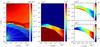 |
Fig. 1 Left panel: density distribution by colour at time t = 5.8 × 10⁴ s in the (quasi)-steady state. The star is located at (r∗,z∗) = (0,4.8 × 1012) cm and the pulsar wind is injected at a distance of 2.4 × 1011 cm with respect the pulsar centre at (rp,zp) = (0,4 × 10¹¹) cm. The grey lines show the obtained streamlines describing the trajectories of the pulsar wind fluid cells; the grey scale and the numbers are only for visualization purposes. Centre panel: distribution by colour of the module of the three-velocity at time t = 5.8 × 10⁴ s in the (quasi)-steady state. Right panel: distribution by colour of the Doppler boosting enhancement (δ4) for the emission produced in the shocked pulsar wind, as seen from 45° (top) and 135° (bottom) from the pulsar-star axis, at time t = 5.8 × 10⁴ s in the (quasi)-steady state. |
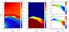 |
Fig. 2 Left panel: density distribution by colour at time t = 0.4 × 10⁴ s (measured from the steady case) considering an inhomogeneous stellar wind with χ = 10 and Rc = 8 × 1010 cm. The remaining plot properties are the same as those in Fig. 1. Centre panel: module of the three-velocity. Right panel: Doppler boosting enhancement as seen from 45° (top) and 135° (bottom). |
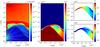 |
Fig. 3 Left panel: density distribution by colour at time t = 1.1 × 10⁴ s (measured from the steady case) considering an inhomogeneous stellar wind with χ = 10 and Rc = 4 × 1011 cm. The remaining plot properties are the same as those in Fig. 1. Centre panel: module of the three-velocity. Right panel: doppler boosting enhancement as seen from 45° (top) and 135° (bottom). |
3. Radiation
3.1. Non-thermal emitter
From the streamline information obtained from the RHD simulations, it is possible to derive the characteristics of injection, cooling, and radiation of the non-thermal particles as they are advected by the shocked pulsar wind. Each streamline is divided into 200 cells and from each cell we have a set of parameters: position and velocity information, pressure (P), density (ρ), streamline effective section (S), magnetic field in the flow frame (B′), and the flow velocity divergence (∇(Γv), for the computation of adiabatic losses; see de la Cita et al. 2016). A tracer accounting for wind mixing, ranging from 0 (100% pulsar material) to 1 (100% stellar wind), is provided by the RHD simulations.
In this work, we consider that the non-thermal emitter is restricted to the shocked pulsar wind, i.e., particles are accelerated at the pulsar wind termination shock, although the unshocked pulsar wind may also be an efficient gamma-ray emitter for certain values of the wind Lorentz factor (e.g. Aharonian & Bogovalov 2003; Khangulyan et al. 2007). For each cell of each streamline, we compute whether there is non-thermal particle injection and the luminosity injected in the form of these particles. The following procedure is applied along each streamline. Starting from the line origin, cells where the internal energy increases (and the flow velocity decreases) are found. Non-thermal particles with total energy corresponding to a fixed fraction ηNT of the internal energy increase are injected in these cells. Particle acceleration in pulsar wind termination shocks is not yet well understood. Our main aim here, however, is just to show general trends in the radiation due to the presence of clumps. Therefore, we follow a purely phenomenological approach, and assume that the injected particles follow a power-law distribution in energy, with a typical index of −2, and two exponential cut-offs at high (Emax) and low (Emin) energies. The value of Emin is fixed to 1 MeV, and Emax is derived adopting an acceleration rate of ~ 0.1 qB′c, typical of efficient accelerators. A value for the fraction ηNT of 0.1 is taken, but all the results scale linearly; currently, this quantity cannot be derived from first principles. We note that, as discussed by Dubus et al. (2015), a large value of ηNT would not be consistent if losses of energy (and momentum; see Sect. 5) were significant in the emitting flow, affecting the flow dynamics. In any case, a formal limitation for ηNT would be a value such that the energy losses of the non-thermal particles in the laboratory frame (LF) should be well below the energy rate of the pulsar wind (i.e. Lp; in fact, ηNT = 0.1 implies radiation losses of a small percentage of Lp; see Sect. 3.2).
Once the injection of non-thermal particles is characterized, we compute the energy evolution and spatial propagation of particles along the streamlines until they leave the grid, which eventually leads to a steady state. Then, the synchrotron and IC emission for each cell, for all the streamlines, are computed in the fluid frame (FF), and appropriately transformed afterwards to the observer frame multiplying the photon energies and fluxes by δ = 1/Γ(1−vcos [φobs]) and δ4, respectively, where φobs is the angle between the flow direction of motion and the line of sight in the LF. A detailed description of the applied method is described in de la Cita et al. (2016), Appendix B.
In the present scenario, the gamma-ray absorption due to electron-positron pair creation in the stellar photon field cannot be neglected and is taken into account. To compute gamma-ray absorption, we have adopted the cross section from Gould & Schréder (1967), and assumed that the star is far enough to be considered point-like (see e.g. Dubus 2006a; Bosch-Ramon & Khangulyan 2009). The angle between the direction of the stellar photons, which come from the star centre, and the observer line of sight, is taken into account for both pair production and IC scattering (see e.g. Aharonian & Atoyan 1981; Khangulyan et al. 2014a, for the latter). With all this information the total spectral energy distributions (SED) and the emission maps of the different radiation channels can be built. To keep the calculations manageable, emission of secondary particles from gamma-ray absorption (i) and IC cascading (ii) has not been considered, but these processes could indeed be important in close binaries, mainly increasing the X-ray fluxes (i; high ambient magnetic field), or enhancing the effective transparency of the system (ii; low ambient magnetic field) (e.g. Sierpowska & Bednarek 2005; Aharonian et al. 2006b; Sierpowska-Bartosik & Torres 2007; Bosch-Ramon et al. 2008; Cerutti et al. 2010; Bosch-Ramon & Khangulyan 2011).
The non-thermal emitter is a 3D structure, whereas the hydrodynamic simulations are 2D. Therefore, the streamlines have to be distributed in azimuthal angle around the pulsar-star axis to properly account for IC, gamma-ray absorption, and Doppler boosting for an observer looking from a certain direction. To do so, an azimuthal random position has been assigned to each streamline cell conserving the values of the r- and z-components for position and velocity. This transformation, only concerned with the observer direction, affects just the radiative part of the code; the particle energy distribution in each cell is determined by axisymmetric processes and remains unaffected.
The companion star is by far the dominant source of target IC photons. The stellar spectrum has been assumed to be typical for an O-type star: a black body with a temperature and luminosity of T⋆ = 4 × 10⁴ K and L⋆ = 1039 erg s-1, respectively. The high stellar luminosity allows us to neglect the radiation field produced in the emitter itself, in particular the role of synchrotron self-Compton radiation, which is a safe assumption as long as L⋆ ≫ Lp/η. The magnetic field is set as specified in Eq. (2) using two values for χB, 10-3 and 0.1, illustrative of a low and a high magnetic field case, respectively. Typically, pulsar winds at termination are thought to be strongly dominated by their kinetic energy (e.g. Kennel & Coroniti 1984; Bogovalov et al. 2012; Aharonian et al. 2012), although some models predict a high magnetization up to the termination shock, where the magnetic field would efficiently dissipate (e.g. Lyubarsky & Kirk 2001). We note that for χB = 0.1 the condition of a negligible magnetic field becomes only marginally fulfilled.
3.2. Results
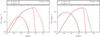 |
Fig. 4 Spectral energy distribution of synchrotron and IC for the no clump scenario, in the low (χB = 10-3) and high (χB = 0.1) magnetic field cases (left and right, respectively). We note that the unabsorbed (thin lines) and the absorbed (thick lines) IC emission are distinguishable only for φ = 45° and 90°. |
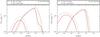 |
Fig. 7 Spectral energy distribution of synchrotron and IC for φ = 90°, in the low (χB = 10-3) and high (χB = 0.1) magnetic field cases (left and right, respectively). |
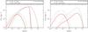 |
Fig. 8 Spectral energy distribution of synchrotron and IC for a fixed magnetic field (low case, χB = 10-3) and different φ-values: 45 and 135° (left and right, respectively). |
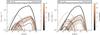 |
Fig. 9 Contribution of each streamline (numbered as in left panel of Fig. 1) to the overall synchrotron (dotted line) and IC (solid line) SED. The no clump (left) and the large clump (right) scenarios are both computed for a low magnetic field (χB = 10-3) and φ = 90°. |
The non-thermal emission was computed for three different stellar wind scenarios: the steady state of the two-wind interaction structure with no clump, the case with a small clump (χ = 10, Rc = 8 × 1010 cm), and the case with a large clump (χ = 10, Rc = 4 × 1011 cm). In addition to considering two magnetic field cases (χB = 10-3 and 0.1), three representative viewing angles were also considered: φ = 45°, 90°, and 135°. The first angle corresponds for instance to the superior conjunction of the compact object (SUPC) and a system inclination of 45°, the second to an intermediate orbital phase, and the third might represent the inferior conjunction (INFC) for the same inclination; the parameter values are listed in Table 2. The simulation times adopted for the emission calculations, of the cases including a clump, were chosen such that the clump was at its closest point from the pulsar; the state of the emitting flow can be considered steady given the short time needed for the particles to leave the grid. For each of these scenarios, we obtained the corresponding synchrotron and IC SEDs. These SEDs are presented in Figs. 4–9, the last of which shows the contribution from each streamline. Figure 10 shows the particle energy distribution in the LF for each streamline, and the summation of all of them. Maps were also computed to show how the emission is distributed in the rz-plane in the shocked pulsar wind region. These maps are presented in Figs. 11 and 12. Figure 13 illustrates the importance of the extended nature of the emitter comparing two SEDs: those obtained for the computed emitter geometry, and those computed assuming that all the emitting cells have the pulsar location (keeping, nonetheless, the particle distributions of the extended emitter). The extended emitter on the scales studied has a minor effect on IC, but a major one in gamma-ray absorption for the represented case with φ = 45°.
Set of parameters for the three scenarios considered.
Values of the integrated emission in different bands for the case of weak magnetization, χB = 10-3, given in erg s-1; and the difference imposed by clumps to the homogeneous case, given in per cent.
The impact of energy losses on the non-thermal particles can be seen by comparing the injected non-thermal luminosities with the energy leaving the computational domain per time unit in the LF. Particles lose 1.6 × 1035 erg s-1 through radiative losses, or a ≈ 23% of the injected non-thermal luminosity in the no clump case; instead, in the large clump case 1.8 × 1035 erg s-1 is radiated, or ≈ 20%. The adiabatic losses have more impact, around 49% of the injected non-thermal luminosity for both no clump and large clump cases. The total injected non-thermal luminosities would be 7.1 × 1035 and 9.1 × 1035 erg s-1 for the cases without a clump and with a large clump, respectively. Doppler boosting shows up by comparing the synchrotron+IC total luminosity in the observer frame for the case without clump, φ = 90° and χB = 10-3, of 2.75 × 1035 erg s-1, with the same quantity in the fluid frame, of 1.2 × 1035 erg s-1, where there is an increase of a factor between 2 and 3 in the emission.
For informative purposes and completeness, we provide in Table 3 the luminosities in the energy bands 1–10 keV, 10–100 keV, 0.1–100 MeV, 0.1–100 GeV, and 0.1–100 TeV for the cases without and with clump, focusing on the low magnetic field case (χB = 10-3), which can be considered the more realistic one (see Sect. 3.1). It is clear that in the system considered, which is representative (Dubus 2013), the radiative cooling represents ~ 1/3 of the injected non-thermal luminosity, and for ηNT = 0.1, a small percentage of Lp. In the large clump case, adiabatic losses get enhanced because of the shrinking of the two-wind interaction region, a tendency previously suggested in Bosch-Ramon (2013). This effect can be seen as a suppression of the lower energy part (where adiabatic losses are important) of the IC spectra in Fig. 7.
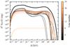 |
Fig. 10 Particle energy distributions for the different streamlines (thin lines) and the sum of all of them (thick black line) in the LF, for the low magnetic field (χB = 10-3) no clump scenario. |
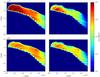 |
Fig. 11 Maps of the bolometric luminosity per cell for the no clump scenario, taking a low magnetic field χB = 10-3. Top panels: map in the rz-plane of the distribution of IC (left) and synchrotron (right) for φ = 45°. Bottom panels: same as the top panels, but for φ = 135°. |
3.3. Applications to PSR B1259-63/LS2883
The binary pulsar system PSR B1259-63/LS2883 consists of a 47.7 ms radio pulsar (Johnston et al. 1992; Kijak et al. 2011) on an eccentric orbit around a luminous O8.5 Ve star (Negueruela et al. 2011). The pulsar orbits are characterized by the following orbital parameters: eccentricity e = 0.87, period Porb = 3.5 yr, and semi-major axis a2 = 6.9 AU (see Negueruela et al. 2011, and references therein). The stellar companion in the system is thought to rapidly rotate (Negueruela et al. 2011). The rotation results in a strong surface temperature gradient (Tpole = 3.4 × 10⁴ K and Teq = 2.75 × 10⁴ K), and in the formation of a circumstellar disc. The plane of the orbit and the disc plane are expected to be misaligned. Negueruela et al. (2011) derived the orbital inclination of iorb ≈ 23° and adopted that the star rotation axis is inclined with respect to the line of sight by 32° (i.e., the star is mostly seen from the pole). Accounting for the uncertainty of the star orientation, the IC emission/loss process can be well approximated by a black body with temperature T∗ = 3 × 10⁴ K (Khangulyan et al. 2011).
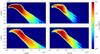 |
Fig. 12 Maps of the bolometric luminosity per cell, for the large clump scenario, taking a low magnetic field χB = 10-3. Top panels: IC (left) and synchrotron radiation (right) for φ = 45°. Bottom panels: same as the top panels, but for φ = 135°. |
The temperature and luminosity of the UV companion correspond to a late O star, but because of the fast rotation a Be star-type disc is formed. Thus the stellar wind in PSR B1259-63/LS2883 should consist of two distinct regions: a dense Keplerian disc, which is crossed by the pulsar approximately −16 and + 18 d to periastron passage and a fast low-density polar wind. The mass-loss rate and density of the discs around Be stars can vary significantly, but the density should be significantly higher than in the polar wind, and the azimuthal velocity should be Keplerian, i.e., vd ~ 2 × 10² km s-1 (at a distance of 1013 cm from the star). Based on the shape of the X-ray light curve, Takata et al. (2012) predicted that the density of the disc base in PSR B1259-63/LS2883 might be very high ρ0 ~ 10-9 g cm-3, but this conclusion is likely the result of large computational uncertainties. The polar wind should be similar to a wind from a O-type star, vw ~ 2 × 10³ km s-1. Both these winds might be inhomogeneous, but the disc clumps can be significantly more massive, so in what follows we consider the possible impact of a disc clump on the non-thermal emission in the system.
The system displays variable broadband non-thermal radio, X-ray, and TeV gamma-ray emission close to periastron passage (Grove et al. 1995; Johnston et al. 2005; Chernyakova et al. 2006, 2014, 2015; Aharonian et al. 2005, 2009; Uchiyama et al. 2009; H.E.S.S. Collaboration et al. 2013; Caliandro et al. 2015; Romoli et al. 2015). Although the light curves of the non-thermal emission clearly diverge in different energy bands, the general tendency is similar. Approximately 30 d to periastron passage the flux starts to increase and reaches its maximum around 20–10 d before periastron passage (depending on the energy band). When the pulsar approaches periastron, a decreasing tendency in the flux level is apparent. In post-periastron epoch the flux increases again, and then gradually decreases. This two-hump structure is less pronounced in the radio band, probably because of the long cooling time of the radio-emitting electrons, and in TeV gamma rays, possibly because of larger data uncertainties. The X-ray light curve displays quite stable orbit-to-orbit behaviour with two clear maxima. The pre- and post-periastron maxima of the X-ray light curve are characterized by similar patterns: a sharp increase and a slower decay, with a larger maximum flux level in the post-periastron epoch (Chernyakova et al. 2015). The X-ray peaking fluxes are reached close to the epochs, when the pulsed radio emission disappears. The weakening of the pulsed emission is conventionally associated with the pulsar eclipse by the circumstellar disc approximately during the epoch (−16, +18) d to periastron passage. The location of the light curve maxima suggests that the circumstellar disc may play an important role in the formation of the non-thermal emission. In turn, as indicated by the change of the equivalent width of Hα (Chernyakova et al. 2015), the pulsar also affects the disc. This complex interplay makes modelling the emission in this system a very challenging task, thus a consistent multi-wavelength interpretation is currently missing (however, see Takata et al. 2012).
In addition to TeV gamma rays, bight GeV flares have been detected from the system with Fermi LAT in 2011 January and 2014 May (see Caliandro et al. 2015, and references therein). In both epochs the onset of the flares occurred approximately one month after periastron passage. During the flare summit the measured GeV luminosity in 2011 was a factor of ~ 1.5 higher than, but the flare duration was similar to, that in 2014 (see e.g. Romoli et al. 2015). The typical flare flux is ~ 10-6 ph cm-2 s-1, which means a GeV output ~ 10% of the pulsar spin-down luminosity (Lp ≈ 8 × 1035 erg s-1, Johnston et al. 1992) for the distance to the system of 2.3 pc (Negueruela et al. 2011). No detectable change in the TeV emission was observed during the onset of the GeV flare in 2011 (H.E.S.S. Collaboration et al. 2013). Hard X-ray emission detected with NuSTAR during the GeV flare suggests that the GeV emission might be generated by the same radiation mechanism as the multi-keV X-ray emission, namely through the synchrotron channel (Tam et al. 2015; Chernyakova et al. 2015).
In what follows we qualitatively consider the possible contribution of the emission generated by the interaction of stellar wind clumps with the pulsar wind to the radiation detected from PSR B1259-63/LS2883, for the GeV flare, and the disc crossing in TeV.
3.3.1. GeV flare
As discussed in Paredes-Fortuny et al. (2015), the GeV flare detected from PSR B1259-63/LS2883 by Fermi LAT could be related to the impact of a dense, large clump of material, probably associated with the decretion disc of the Be star (Chernyakova et al. 2014). This GeV flare seems to follow a repetitive pattern (e.g. Caliandro et al. 2015; Chernyakova et al. 2015), which in the scenario just sketched would imply that the disc is similarly affected orbit to orbit, and parts of it are torn apart and directed towards the pulsar. The ram pressure of such a piece of circumstellar disc could have a strong impact on the two-wind interaction structure. As shown by Paredes-Fortuny et al. (2015), just a small fraction of the disc mass in the form of a clump of matter would be enough to strongly reduce the size of the interaction region. As was outlined above, the flare onset occurs approximately two weeks after the reappearance of the pulsed radio signal, and thus the pulsar has moved relatively far from the disc. We nevertheless assume that a dense cloud can still collide with the pulsar wind at this epoch.
The arrival of a large, dense piece of disc could potentially enhance, by compressing the emitting region, the energy density of the local radiation field (e.g. X-rays from the collision region, Dubus & Cerutti 2013; see also Khangulyan et al. 2012 for a related scenario based on IR target photons) to a point when synchrotron self-Compton (SSC) becomes dominant over external IC. This process seems nevertheless unlikely in PSR B1259-63/LS2883. Given the pulsar spin-down and the stellar luminosities (L∗ ≈ 3 × 1038 erg s-1, Negueruela et al. 2011), even optimistically assuming that most of Lp goes to the target photons for SSC, adopting the Thomson approximation for IC, and neglecting IC angular effects, to increase the local photon energy density above the stellar level, the two-wind interaction region should become ≲1/40 times the size typically considered. This is ~ 10% of the pulsar-star separation distance (Dubus & Cerutti 2013 obtained a similarly small emitting region). Although a detailed account of this possibility is still not available, such a huge reduction in size requires an increase in stellar material ram pressure by several orders of magnitude and does not seem plausible.
The arrival of a clump may by itself be enough to substantially enhance the IC emission for a combination of Doppler boosting, pulsar wind shock obliqueness, etc. To check this possibility, we computed the emission of the steady and the large clump cases adopting the parameters of PSR B1259-63/LS2883 at the time of the flare in GeV (not shown here). We took the orbital phase to be around the inferior conjunction of the compact object, an inclination of 23°, and scaled the hydrodynamic solution (Paredes-Fortuny et al. 2015) to a star-pulsar separation distance in accordance with the source properties. This scaling yields a clump mass ~ 1021 g, and a clump destruction time of about a week (the actual flare lasted for a few weeks). For instance, in the low B case, a jump in gamma-ray luminosity by a factor of ~ 2 was obtained, not far from the difference between the flare and the periastron Fermi LAT luminosity in PSR B1259-63/LS2883 (e.g. Caliandro et al. 2015). Unfortunately, the energetics in our case was short by about two orders of magnitude, even when adopting χNT = 1. Therefore, the simulated scenario is, in its present form, far from being able to explain the GeV flare in PSR B1259-63/LS2883.
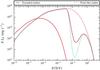 |
Fig. 13 Spectral energy distribution of the synchrotron and IC emission in the no clump scenario, with φ = 45° and χB = 10-3. The emission for the computed emitter geometry (solid line) and that obtained assuming that the emitter is point-like (dashed line) are shown. The lower energy component corresponds to synchrotron emission. |
3.3.2. Disc crossing and TeV emission
We also studied the interaction of the pulsar wind with the Be star disc assuming that this may be roughly approximated as the encounter between the wind and a large inhomogeneity. From a hydrodynamical point of view, as shown in Okazaki et al. (2011), the disc may be of great dynamical importance for the geometry of the pulsar wind termination shock, and thus in the overall non-thermal emitting region (see Takata et al. 2012, for non-relativistic calculations without particle energy losses). The effects of the disc in the non-thermal emission in PSR B1259-63/LS2883 has already been discussed, for instance in Khangulyan et al. (2007; see also Chernyakova et al. 2006).
We computed the SED for both the steady and the large clump cases when the pulsar is supposed to cross the Be disc after periastron passage. Assuming that the beginning of the disc crossing could be roughly modelled by the encounter with a large clump, we tried to semi-quantitatively reproduce the energetics and increase in flux above 100 GeV observed around those orbital phases. As the results were slightly improved, and given the inclination uncertainty, we adopted i = 30° instead of 23°. As shown in Fig. 14, with minor changes in the calculation set-up and a little parameter tuning (ηNT = 1; χB = 10-3)3, similar flux levels and evolution (a rise by a factor of several) are obtained, although with a somewhat steeper spectrum than the average one given in Romoli et al. (2015).
4. Conclusions
The results shown in Figs. 4–10 are partially determined by several well-known effects. First, there is a competition between synchrotron and IC losses at particle energies high enough for radiation cooling to dominate over adiabatic losses. Different magnetic-to-target radiation energy density ratios yield different synchrotron-to-IC luminosity ratios. Dominant synchrotron or IC in the Thomson regime (for IC photons ≲10 GeV) lead to a spectral softening, whereas dominant IC in Klein Nishina (for IC photons ≳10 GeV) leads to a spectral hardening (e.g. Khangulyan & Aharonian 2005). Second, an important factor is IC scattering on an anisotropic target photon field, which softens and boosts the gamma-ray emission for close to head-on collisions (around SUPC), and hardens and reduces the gamma-ray emission for small scattering angles (around INFC) (e.g. Khangulyan et al. 2008; Dubus et al. 2008). Third, at the highest energies there is absorption through pair creation in the anisotropic photon field of the star. This process has its minimum threshold energy of the absorbed gamma rays (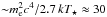 GeV), and the strongest attenuation, for close to head-on collisions (around SUPC), whereas it presents a high absorption threshold, and weak attenuation, for small photon-photon interaction angles (around INFC) (e.g. Böttcher & Dermer 2005; Dubus 2006a; Khangulyan et al. 2008). For the adopted stellar luminosity and orbital separation distance, gamma-ray absorption around 1 TeV is very strong for φ < 90°. This suggests that the bright TeV emission detected from several close binary systems, e.g. LS 5039 (Aharonian et al. 2006a), cannot be entirely generated in the inner part of the colliding wind structure, and some additional production sites should be considered (Zabalza et al. 2013).
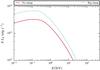 |
Fig. 14 Comparison of the spectral energy distribution for the steady and the large clump case adapting the hydrodynamical results to the case of PSR B1259-63/LS2883 around 20 d after periastron, roughly at the second disc passage. |
The importance of synchrotron losses was discussed in Bosch-Ramon (2013) in the context of a clump large enough to significantly reduce the size of the two-wind interaction region, which is expected to enhance the magnetic field in the shocked pulsar wind. This effect is seen in our results (see Table 3) when comparing the synchrotron and IC luminosities in different energy bands, and in the absence or presence of clumps. Adiabatic losses are also increased by the reduction of the two-wind interaction region, as noted in Sect. 3.2.
Doppler boosting is a very important factor characterizing the observer synchrotron and IC luminosities (by δ4), and to a lesser extent spectra through photon energy boosting (by δ), in the scenario studied here. Doppler boosting has been already discussed (e.g. Khangulyan et al. 2008, 2014b; Dubus et al. 2010, 2015; Kong et al. 2012; del Palacio et al. 2015) in the framework of a homogeneous stellar wind; in this context we obtain similar results, as Doppler boosting induces luminosity variations of up to a factor of a few by comparing different viewing angles in certain bands (see Table 3, no clump scenario). Radiation enhancement in the cases computed here is well illustrated by the maps presented in the right panels of Figs. 1–3. For comparison, the impact of clump absence/presence is also shown in the left panel of Figs. 1–3 for the general direction of the streamlines, and in the central panel of the same figures. for the shocked pulsar wind speed distribution. The effects on radiation are seen in the SEDs and maps shown in Figs. 11 and 12 (and again in Table 3, comparing the same energy bands and φ values for the three cases).
If the stellar wind is homogeneous, the two-wind interaction structure is already prone to suffer hydrodynamical instabilities (e.g. Bosch-Ramon et al. 2012, 2015; Lamberts et al. 2013; Paredes-Fortuny et al. 2015), i.e. the tinniest irregularities in the wind act as inhomogeneity seeds. The corresponding dispersion in the velocity field coupled with Doppler boosting can thus introduce a chaotic variability component to the emission even in the absence of clumps. Therefore, even rather small clumps enhance instability formation and growth, making the emission variability more complex.
It is interesting to compare the cases without and with a small clump in Table 3 for the same viewing angle. In these two cases, the overall two-wind interaction structure does not change significantly, and the flux difference is determined by the perturbations in the flow velocity. This already leads to luminosity variations of almost a factor of ~ 2 in certain bands. Large clumps add perturbations to the shocked flow structure, and also change the overall distribution of the streamline directions as the shock approaches the pulsar significantly. This induces a characteristic pattern, with its evolution determined by the shocked clump dynamics. We note that in the more realistic case of using a 3D simulation to compute the emission, the lack of symmetry in the azimuthal direction with respect to the pulsar-star axis would likely lead to an even more chaotic velocity field, and thus to stronger differences between clump scenarios.
It is worth noting that the shock becomes more perpendicular when approaching the pulsar in the large clump case. Therefore, the transfer of energy to non-thermal particles is increased, and thus the clump presence enhances particle acceleration at the pulsar wind shock, as shown by the injected luminosity into non-thermal particles, which in the large clump case is ~ 50% larger than without a clump (see Sect. 3.2). However, this effect may be difficult to disentangle from Doppler boosting in the radiation results. Also, if magnetic field reconnection plays a sensible role in particle acceleration, chaotic perturbations of the magnetic field structure induced by clumps may have a strong impact on the particle acceleration (Sironi & Spitkovsky 2011).
From a direct application of our radiation calculations using hydrodynamical information about the post-periastron GeV flare, and the post-periastron disc crossing in TeV, in PSR B1259-63/LS2883, the former is hard to reproduce in our simplified scenario, whereas the second semi-quantitatively agrees with our results.
5. Final remarks
This work provides some illustrative examples of how different types of clumps can affect the emitting region and the radiation itself in the case of an inhomogeneous stellar wind interacting with a pulsar wind. The studied effects (clump presence, velocity field dispersion, Doppler boosting for a given observer, instability development, magnetic field increase, and closing of the pulsar wind shock) acting together can either cancel out to some extent or combine rather unpredictably. There are also many different timescales, as instability growth, region shrinking, and magnetic field growth depend on the clump evolution timescale, which itself depends to first order on the clump size and density. On the other hand, the shocked pulsar wind flow can change direction much more quickly, and the rapidly changing, non-uniform, beaming of radiation in the emitting region is an important factor shaping variability. One can thus conclude that flares could occasionally be seen in some or all bands of the spectrum, with their duration determined by the dominant variability origin, whereas in general emission may vary more smoothly. There are periodic emission features in the systems studied that originate in repetitive physical phenomena (e.g. orbit-related IC, orbit-related Doppler boosting, pair creation angular effects, changes in radiative and non-radiative cooling along the orbit, etc.), but non-periodic variability originates from a combination of different, equally important, factors, and they can be hard to disentangle. A study of the X-ray light curve can provide information on the different processes shaping the non-thermal emission. We note that Kishishita et al. (2009) have found that the X-ray light curve of the pulsar binary candidate LS 5039 in the years 1999–2007 was rather stable, with even fine structures such as spikes and dips similar from one orbit to another. This non-chaotic behaviour, if confirmed, would not be explained by the processes discussed in this work.
A quantitative assessment of the importance of the different factors in the clump wind scenario is the next step to be carried out. The reason is that the shocked pulsar wind accelerates as it propagates (e.g. Bogovalov et al. 2008), and it does so in parallel with instability growth. Therefore, a quantitative prediction of the impact of instability growth on the emission, induced either by small perturbations or large clumps, requires a larger computational grid to properly capture all these processes. Multiple clump interactions should be also simulated. In this regard, a stellar wind with a distribution of clump properties (e.g. Moffat 2008) is likely to be an additional variability source affecting the non-linear hydrodynamical processes occurring in the two-wind interaction structure. Finally, the dynamical role of the magnetic field cannot be forgotten if the pulsar wind is weakly magnetized, as the flow magnetization may significantly grow in specific regions of the shocked pulsar wind (see e.g. Fig. 6 in Bogovalov et al. 2012)4. This growth can be important enough to moderate the development of hydrodynamical instabilities, or induce anisotropy and thus further complexity to their development.
If non-thermal radiation losses were to be accounted for (say ηNT ≲ 1) when modelling the properties of the shocked pulsar wind, full radiation-(magneto)hydrodynamic simulations should be carried out. We must point out though that, in addition to this effect, it is also necessary to account for the fact that IC emission on stellar photons is already anisotropic in the FF. This anisotropy in the FF implies that there will be momentum lost in the direction of the star, a form of Compton rocket (e.g. Odell 1981). Thus, if IC radiation is important for the flow internal (non-thermal) energy losses, its dynamical impact will also be important for the emitting flow through the loss of momentum in specific directions. Synchrotron emission may also be anisotropic if the magnetic field is ordered, but unless the field presents a strong gradient emission by particles moving in opposite directions along the field lines would effectively cancel the momentum loss out.
Acknowledgments
We thank the anonymous referee for the constructive and useful comments. We acknowledge support by the Spanish Ministerio de Economía y Competitividad (MINECO) under grants AYA2013-47447-C3-1-P, and MDM-2014-0369 of ICCUB (Unidad de Excelencia “María de Maeztu”) and the Catalan DEC grant 2014 SGR 86. This research has been supported by the Marie Curie Career Integration Grant 321520. V.B.-R. also acknowledges financial support from MINECO and European Social Funds through a Ramón y Cajal fellowship. X.P.-F. also acknowledges financial support from Universitat de Barcelona and Generalitat de Catalunya under grants APIF and FI (2015FI_B1 00153), respectively. D.K. acknowledges support from the Russian Science Foundation under grant 16-12-10443. M.P. is a member of the working team of projects AYA2013-40979-P and AYA2013-48226-C3-2-P, funded by MINECO.
References
- Aharonian, F. A., & Atoyan, A. M. 1981, Ap&SS, 79, 321 [NASA ADS] [Google Scholar]
- Aharonian, F. A., & Bogovalov, S. V. 2003, New Astron., 8, 85 [NASA ADS] [CrossRef] [Google Scholar]
- Aharonian, F., Akhperjanian, A. G., Aye, K.-M., et al. 2005, A&A, 442, 1 [NASA ADS] [CrossRef] [EDP Sciences] [Google Scholar]
- Aharonian, F., Akhperjanian, A. G., Bazer-Bachi, A. R., et al. 2006a, A&A, 460, 743 [NASA ADS] [CrossRef] [EDP Sciences] [Google Scholar]
- Aharonian, F., Anchordoqui, L., Khangulyan, D., & Montaruli, T. 2006b, J. Phys. Conf. Ser., 39, 408 [NASA ADS] [CrossRef] [Google Scholar]
- Aharonian, F., Akhperjanian, A. G., Anton, G., et al. 2009, A&A, 507, 389 [NASA ADS] [CrossRef] [EDP Sciences] [Google Scholar]
- Aharonian, F. A., Bogovalov, S. V., & Khangulyan, D. 2012, Nature, 482, 507 [NASA ADS] [CrossRef] [PubMed] [Google Scholar]
- Bogovalov, S. V., Khangulyan, D. V., Koldoba, A. V., Ustyugova, G. V., & Aharonian, F. A. 2008, MNRAS, 387, 63 [NASA ADS] [CrossRef] [Google Scholar]
- Bogovalov, S. V., Khangulyan, D., Koldoba, A. V., Ustyugova, G. V., & Aharonian, F. A. 2012, MNRAS, 419, 3426 [NASA ADS] [CrossRef] [Google Scholar]
- Bosch-Ramon, V. 2011, ArXiv e-prints [arXiv:1103.2996] [Google Scholar]
- Bosch-Ramon, V. 2013, A&A, 560, A32 [NASA ADS] [CrossRef] [EDP Sciences] [Google Scholar]
- Bosch-Ramon, V., & Khangulyan, D. 2009, Int. J. Mod. Phys. D, 18, 347 [NASA ADS] [CrossRef] [Google Scholar]
- Bosch-Ramon, V., & Khangulyan, D. 2011, PASJ, 63, 1023 [NASA ADS] [Google Scholar]
- Bosch-Ramon, V., Khangulyan, D., & Aharonian, F. A. 2008, A&A, 482, 397 [Google Scholar]
- Bosch-Ramon, V., Barkov, M. V., Khangulyan, D., & Perucho, M. 2012, A&A, 544, A59 [NASA ADS] [CrossRef] [EDP Sciences] [Google Scholar]
- Bosch-Ramon, V., Barkov, M. V., & Perucho, M. 2015, A&A, 577, A89 [NASA ADS] [CrossRef] [EDP Sciences] [Google Scholar]
- Böttcher, M., & Dermer, C. D. 2005, ApJ, 634, L81 [NASA ADS] [CrossRef] [Google Scholar]
- Bucciantini, N., Amato, E., & Del Zanna, L. 2005, A&A, 434, 189 [NASA ADS] [CrossRef] [EDP Sciences] [Google Scholar]
- Caliandro, G. A., Cheung, C. C., Li, J., et al. 2015, ApJ, 811, 68 [NASA ADS] [CrossRef] [Google Scholar]
- Cerutti, B., Malzac, J., Dubus, G., & Henri, G. 2010, A&A, 519, A81 [NASA ADS] [CrossRef] [EDP Sciences] [Google Scholar]
- Chernyakova, M., Neronov, A., Lutovinov, A., Rodriguez, J., & Johnston, S. 2006, MNRAS, 367, 1201 [NASA ADS] [CrossRef] [Google Scholar]
- Chernyakova, M., Abdo, A. A., Neronov, A., et al. 2014, MNRAS, 439, 432 [NASA ADS] [CrossRef] [Google Scholar]
- Chernyakova, M., Neronov, A., van Soelen, B., et al. 2015, MNRAS, 454, 1358 [NASA ADS] [CrossRef] [Google Scholar]
- Colella, P., & Woodward, P. R. 1984, J. Comput. Phys., 54, 174 [NASA ADS] [CrossRef] [MathSciNet] [Google Scholar]
- de la Cita, V. M., Bosch-Ramon, V., Paredes-Fortuny, X., Khangulyan, D., & Perucho, M. 2016, A&A, 591, A15 [NASA ADS] [CrossRef] [EDP Sciences] [Google Scholar]
- del Palacio, S., Bosch-Ramon, V., & Romero, G. E. 2015, A&A, 575, A112 [NASA ADS] [CrossRef] [EDP Sciences] [Google Scholar]
- Donat, R., & Marquina, A. 1996, J. Comput. Phys., 125, 42 [NASA ADS] [CrossRef] [Google Scholar]
- Donat, R., Font, J. A., Ibáñez, J. M. l., & Marquina, A. 1998, J. Comput. Phys., 146, 58 [NASA ADS] [CrossRef] [Google Scholar]
- Dubus, G. 2006a, A&A, 451, 9 [NASA ADS] [CrossRef] [EDP Sciences] [Google Scholar]
- Dubus, G. 2006b, A&A, 456, 801 [NASA ADS] [CrossRef] [EDP Sciences] [Google Scholar]
- Dubus, G. 2013, A&ARv, 21, 64 [NASA ADS] [CrossRef] [Google Scholar]
- Dubus, G., & Cerutti, B. 2013, A&A, 557, A127 [NASA ADS] [CrossRef] [EDP Sciences] [Google Scholar]
- Dubus, G., Cerutti, B., & Henri, G. 2008, A&A, 477, 691 [NASA ADS] [CrossRef] [EDP Sciences] [Google Scholar]
- Dubus, G., Cerutti, B., & Henri, G. 2010, A&A, 516, A18 [NASA ADS] [CrossRef] [EDP Sciences] [Google Scholar]
- Dubus, G., Lamberts, A., & Fromang, S. 2015, A&A, 581, A27 [NASA ADS] [CrossRef] [EDP Sciences] [Google Scholar]
- Font, J. A., Ibanez, J. M., Marquina, A., & Marti, J. M. 1994, A&A, 282, 304 [NASA ADS] [Google Scholar]
- Gould, R. J., & Schréder, G. P. 1967, Phys. Rev., 155, 1404 [NASA ADS] [CrossRef] [Google Scholar]
- Grove, J. E., Tavani, M., Purcell, W. R., et al. 1995, ApJ, 447, L113 [NASA ADS] [CrossRef] [Google Scholar]
- H.E.S.S. Collaboration, Abramowski, A., Acero, F., et al. 2013, A&A, 551, A94 [NASA ADS] [CrossRef] [EDP Sciences] [Google Scholar]
- Johnston, S., Manchester, R. N., Lyne, A. G., et al. 1992, ApJ, 387, L37 [NASA ADS] [CrossRef] [Google Scholar]
- Johnston, S., Ball, L., Wang, N., & Manchester, R. N. 2005, MNRAS, 358, 1069 [NASA ADS] [CrossRef] [Google Scholar]
- Kennel, C. F., & Coroniti, F. V. 1984, ApJ, 283, 710 [NASA ADS] [CrossRef] [Google Scholar]
- Khangulyan, D., & Aharonian, F. 2005, in High Energy Gamma-Ray Astronomy, eds. F. A. Aharonian, H. J. Völk, & D. Horns, AIP Conf. Ser., 745, 359 [Google Scholar]
- Khangulyan, D., Hnatic, S., Aharonian, F., & Bogovalov, S. 2007, MNRAS, 380, 320 [NASA ADS] [CrossRef] [Google Scholar]
- Khangulyan, D., Aharonian, F., & Bosch-Ramon, V. 2008, MNRAS, 383, 467 [NASA ADS] [CrossRef] [Google Scholar]
- Khangulyan, D., Aharonian, F. A., Bogovalov, S. V., & Ribó, M. 2011, ApJ, 742, 98 [NASA ADS] [CrossRef] [Google Scholar]
- Khangulyan, D., Aharonian, F. A., Bogovalov, S. V., & Ribó, M. 2012, ApJ, 752, L17 [NASA ADS] [CrossRef] [Google Scholar]
- Khangulyan, D., Aharonian, F. A., & Kelner, S. R. 2014a, ApJ, 783, 100 [NASA ADS] [CrossRef] [Google Scholar]
- Khangulyan, D., Bogovalov, S. V., & Aharonian, F. A. 2014b, Int. J. Mod. Phys. Conf. Ser., 28, 1460169 [NASA ADS] [CrossRef] [Google Scholar]
- Kijak, J., Dembska, M., Lewandowski, W., Melikidze, G., & Sendyk, M. 2011, MNRAS, 418, L114 [NASA ADS] [CrossRef] [Google Scholar]
- Kishishita, T., Tanaka, T., Uchiyama, Y., & Takahashi, T. 2009, ApJ, 697, L1 [NASA ADS] [CrossRef] [Google Scholar]
- Kong, S. W., Cheng, K. S., & Huang, Y. F. 2012, ApJ, 753, 127 [NASA ADS] [CrossRef] [Google Scholar]
- Lamberts, A., Fromang, S., Dubus, G., & Teyssier, R. 2013, A&A, 560, A79 [NASA ADS] [CrossRef] [EDP Sciences] [Google Scholar]
- Lucy, L. B., & Solomon, P. M. 1970, ApJ, 159, 879 [NASA ADS] [CrossRef] [Google Scholar]
- Lyubarsky, Y., & Kirk, J. G. 2001, ApJ, 547, 437 [NASA ADS] [CrossRef] [Google Scholar]
- Maraschi, L., & Treves, A. 1981, MNRAS, 194, 1 [Google Scholar]
- Martí, J. M., & Müller, E. 2015, Liv. Rev. Comput. Astrophys., 1, 3 [NASA ADS] [CrossRef] [Google Scholar]
- Martí, J. M., Müller, E., Font, J. A., Ibáñez, J. M., & Marquina, A. 1997, ApJ, 479, 151 [NASA ADS] [CrossRef] [Google Scholar]
- Moffat, A. F. J. 2008, in Clumping in Hot-Star Winds, eds. W.-R. Hamann, A. Feldmeier, & L. M. Oskinova, 17 [Google Scholar]
- Morlino, G., Lyutikov, M., & Vorster, M. 2015, MNRAS, 454, 3886 [NASA ADS] [CrossRef] [Google Scholar]
- Negueruela, I., Ribó, M., Herrero, A., et al. 2011, ApJ, 732, L11 [NASA ADS] [CrossRef] [Google Scholar]
- Odell, S. L. 1981, ApJ, 243, L147 [NASA ADS] [CrossRef] [Google Scholar]
- Okazaki, A. T., Nagataki, S., Naito, T., et al. 2011, PASJ, 63, 893 [NASA ADS] [Google Scholar]
- Olmi, B., Del Zanna, L., Amato, E., Bandiera, R., & Bucciantini, N. 2014, MNRAS, 438, 1518 [NASA ADS] [CrossRef] [Google Scholar]
- Paredes-Fortuny, X., Bosch-Ramon, V., Perucho, M., & Ribó, M. 2015, A&A, 574, A77 [NASA ADS] [CrossRef] [EDP Sciences] [Google Scholar]
- Perucho, M., Hanasz, M., Martí, J. M., & Sol, H. 2004, A&A, 427, 415 [NASA ADS] [CrossRef] [EDP Sciences] [Google Scholar]
- Perucho, M., Martí, J. M., & Hanasz, M. 2005, A&A, 443, 863 [NASA ADS] [CrossRef] [EDP Sciences] [Google Scholar]
- Porth, O., Komissarov, S. S., & Keppens, R. 2014, MNRAS, 438, 278 [NASA ADS] [CrossRef] [Google Scholar]
- Romoli, C., Bordas, P., Mariaud, C., et al. 2015, ArXiv e-prints [arXiv:1509.03090] [Google Scholar]
- Shu, C.-W., & Osher, S. 1988, J. Comput. Phys., 77, 439 [Google Scholar]
- Sierpowska, A., & Bednarek, W. 2005, MNRAS, 356, 711 [NASA ADS] [CrossRef] [Google Scholar]
- Sierpowska-Bartosik, A., & Torres, D. F. 2007, ApJ, 671, L145 [NASA ADS] [CrossRef] [Google Scholar]
- Sironi, L., & Spitkovsky, A. 2011, ApJ, 741, 39 [NASA ADS] [CrossRef] [Google Scholar]
- Takata, J., Okazaki, A. T., Nagataki, S., et al. 2012, ApJ, 750, 70 [NASA ADS] [CrossRef] [Google Scholar]
- Tam, P. H. T., Li, K. L., Takata, J., et al. 2015, ApJ, 798, L26 [NASA ADS] [CrossRef] [Google Scholar]
- Tavani, M., Arons, J., & Kaspi, V. M. 1994, ApJ, 433, L37 [NASA ADS] [CrossRef] [Google Scholar]
- Uchiyama, Y., Tanaka, T., Takahashi, T., Mori, K., & Nakazawa, K. 2009, ApJ, 698, 911 [NASA ADS] [CrossRef] [Google Scholar]
- Volpi, D., Del Zanna, L., Amato, E., & Bucciantini, N. 2008, A&A, 485, 337 [NASA ADS] [CrossRef] [EDP Sciences] [Google Scholar]
- Yoon, D., & Heinz, S. 2017, MNRAS, 464, 3297 [NASA ADS] [CrossRef] [Google Scholar]
- Zabalza, V., Bosch-Ramon, V., Aharonian, F., & Khangulyan, D. 2013, A&A, 551, A17 [NASA ADS] [CrossRef] [EDP Sciences] [Google Scholar]
All Tables
Values of the integrated emission in different bands for the case of weak magnetization, χB = 10-3, given in erg s-1; and the difference imposed by clumps to the homogeneous case, given in per cent.
All Figures
|
Fig. 1 Left panel: density distribution by colour at time t = 5.8 × 10⁴ s in the (quasi)-steady state. The star is located at (r∗,z∗) = (0,4.8 × 1012) cm and the pulsar wind is injected at a distance of 2.4 × 1011 cm with respect the pulsar centre at (rp,zp) = (0,4 × 10¹¹) cm. The grey lines show the obtained streamlines describing the trajectories of the pulsar wind fluid cells; the grey scale and the numbers are only for visualization purposes. Centre panel: distribution by colour of the module of the three-velocity at time t = 5.8 × 10⁴ s in the (quasi)-steady state. Right panel: distribution by colour of the Doppler boosting enhancement (δ4) for the emission produced in the shocked pulsar wind, as seen from 45° (top) and 135° (bottom) from the pulsar-star axis, at time t = 5.8 × 10⁴ s in the (quasi)-steady state. |
| In the text | |
|
Fig. 2 Left panel: density distribution by colour at time t = 0.4 × 10⁴ s (measured from the steady case) considering an inhomogeneous stellar wind with χ = 10 and Rc = 8 × 1010 cm. The remaining plot properties are the same as those in Fig. 1. Centre panel: module of the three-velocity. Right panel: Doppler boosting enhancement as seen from 45° (top) and 135° (bottom). |
| In the text | |
|
Fig. 3 Left panel: density distribution by colour at time t = 1.1 × 10⁴ s (measured from the steady case) considering an inhomogeneous stellar wind with χ = 10 and Rc = 4 × 1011 cm. The remaining plot properties are the same as those in Fig. 1. Centre panel: module of the three-velocity. Right panel: doppler boosting enhancement as seen from 45° (top) and 135° (bottom). |
| In the text | |
|
Fig. 4 Spectral energy distribution of synchrotron and IC for the no clump scenario, in the low (χB = 10-3) and high (χB = 0.1) magnetic field cases (left and right, respectively). We note that the unabsorbed (thin lines) and the absorbed (thick lines) IC emission are distinguishable only for φ = 45° and 90°. |
| In the text | |
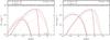 |
Fig. 5 Same as Fig. 4, but for the small clump scenario (χ = 10, Rc = 8 × 1010 cm). |
| In the text | |
 |
Fig. 6 Same as Fig. 4, but for the large clump scenario (χ = 10, Rc = 4 × 1011 cm). |
| In the text | |
|
Fig. 7 Spectral energy distribution of synchrotron and IC for φ = 90°, in the low (χB = 10-3) and high (χB = 0.1) magnetic field cases (left and right, respectively). |
| In the text | |
|
Fig. 8 Spectral energy distribution of synchrotron and IC for a fixed magnetic field (low case, χB = 10-3) and different φ-values: 45 and 135° (left and right, respectively). |
| In the text | |
|
Fig. 9 Contribution of each streamline (numbered as in left panel of Fig. 1) to the overall synchrotron (dotted line) and IC (solid line) SED. The no clump (left) and the large clump (right) scenarios are both computed for a low magnetic field (χB = 10-3) and φ = 90°. |
| In the text | |
|
Fig. 10 Particle energy distributions for the different streamlines (thin lines) and the sum of all of them (thick black line) in the LF, for the low magnetic field (χB = 10-3) no clump scenario. |
| In the text | |
|
Fig. 11 Maps of the bolometric luminosity per cell for the no clump scenario, taking a low magnetic field χB = 10-3. Top panels: map in the rz-plane of the distribution of IC (left) and synchrotron (right) for φ = 45°. Bottom panels: same as the top panels, but for φ = 135°. |
| In the text | |
|
Fig. 12 Maps of the bolometric luminosity per cell, for the large clump scenario, taking a low magnetic field χB = 10-3. Top panels: IC (left) and synchrotron radiation (right) for φ = 45°. Bottom panels: same as the top panels, but for φ = 135°. |
| In the text | |
|
Fig. 13 Spectral energy distribution of the synchrotron and IC emission in the no clump scenario, with φ = 45° and χB = 10-3. The emission for the computed emitter geometry (solid line) and that obtained assuming that the emitter is point-like (dashed line) are shown. The lower energy component corresponds to synchrotron emission. |
| In the text | |
|
Fig. 14 Comparison of the spectral energy distribution for the steady and the large clump case adapting the hydrodynamical results to the case of PSR B1259-63/LS2883 around 20 d after periastron, roughly at the second disc passage. |
| In the text | |
Current usage metrics show cumulative count of Article Views (full-text article views including HTML views, PDF and ePub downloads, according to the available data) and Abstracts Views on Vision4Press platform.
Data correspond to usage on the plateform after 2015. The current usage metrics is available 48-96 hours after online publication and is updated daily on week days.
Initial download of the metrics may take a while.