| Issue |
A&A
Volume 597, January 2017
|
|
|---|---|---|
| Article Number | A95 | |
| Number of page(s) | 12 | |
| Section | Stellar structure and evolution | |
| DOI | https://doi.org/10.1051/0004-6361/201629651 | |
| Published online | 10 January 2017 | |
EPIC 211779126: a rare hybrid pulsating subdwarf B star richly pulsating in both pressure and gravity modes
1 Uniwersytet Pedagogiczny, Obserwatorium na Suhorze, ul. Podchorążych 2, 30-084 Kraków, Poland
e-mail: This email address is being protected from spambots. You need JavaScript enabled to view it.
2 Department of Physics, Astronomy, and Materials Science, Missouri State University, Springfield, MO 65804, USA
3 Nordic Optical Telescope, Rambla José Ana Fernández Pérez 7, 38711 Breña Baja, Spain
4 Armagh Observatory, College Hill, Armagh BT61 9DG, UK
5 School of Physics, Trinity College Dublin, College Green, Dublin 2, Ireland
Received: 5 September 2016
Accepted: 11 October 2016
Abstract
We present our analysis of EPIC 211779126, a pulsating subdwarf B star discovered with the Kepler spacecraft during K2 Campaign 5. We found 154 frequencies in the g-mode region as well as 29 frequencies in the p-mode region. This makes EPIC 211779126 a rare hybrid pulsator with a rich pulsation spectrum in both regions. We successfully identified modal degrees and relative radial orders of most of the g-modes using asymptotic period spacing, and modal degrees of some of the p-modes using rotational splitting. We detected trapped modes, which are a very important feature for constraining theoretical models. Our ground-based spectroscopic observations revealed no companion, therefore EPIC 211779126 is likely a single sdB star. Using p-mode multiplets, we derived a rotation period of approximately 16 days, making EPIC 211779126 the fastest rotating non-binary subdwarf B pulsator observed with Kepler. However, we do not find any resolved multiplets among the high-amplitude g-mode pulsations that correspond to the rotation rate inferred from the p-mode splittings. This may indicate that the star’s core is rotating more slowly than its envelope.
Key words: subdwarfs / stars: oscillations
© ESO, 2017
1. Introduction
Subdwarf B (sdB) stars are hot, low-mass and compact stars located on the blue-ward extension of the horizontal branch. Their temperatures are between 20 000 and 40 000 K, their masses are sharply focused around 0.47 M⊙ (Fontaine et al. 2012), and their radii are between 0.1 and 0.3 R⊙. The formation and evolution of sdB stars, especially single sdB stars, is not fully understood. A star with initial mass less than 2 M⊙ must lose all of its hydrogen envelope shortly before reaching the tip of the red giant branch in order to become a core helium burning star with a negligible hydrogen envelope (Heber 2016). The mechanism of that loss is still under investigation. The sdB star burns helium into carbon in its core and when helium is exhausted, the star proceeds to the white dwarf cooling track, skipping the asymptotic giant branch.
Subdwarf B stars were classified based on analyses of spectroscopic data and from photometry of sdB stars in binaries. Such knowledge is limited to atmospheric properties, including chemical abundances, and bulk parameters of entire stars, such as Teff, radius, or mass. In the 1990s, an unexpected discovery (Kilkenny et al. 1997) as well as independent work on models of sdB stars (Charpinet et al. 1997) revealed that these objects can, and do, drive stellar pulsations. Pulsating sdB (sdBV) stars allow us to study their interiors by building evolutionary models that can be tested observationally. As part of our observational constraints, we supply mode identifications, which describe the pulsation geometry. This is equivalent to finding values for the three parameters n, l, and m. Mode identification is not an easy task. Since, we do not resolve stellar disks, we have to rely on indirect methods, which use rotational multiplets or asymptotic relations; features in amplitude spectra that are rarely seen from ground-based data. Data collected with the Kepler spacecraft, on the other hand, are precise and of sufficient duration that those features have become frequently detected (Reed et al. 2011; Baran & Østensen 2013).
During the Kepler mission, almost 20 new sdBV stars were observed and analyzed. Those analyses revealed important, sometimes new, and unexpected features, such as Doppler boosting (Telting et al. 2012), the lack of multiplets (Baran et al. 2015a), mode trapping (Østensen et al. 2014a), very unstable modes (Østensen et al. 2014b), and internal differential rotation (Foster et al. 2015). A failure of two reaction wheels terminated the original mission, and further use of Kepler required the spacecraft to be repointed at different fields along the ecliptic approximately every 80 days. This current mission is called K2, during which, we can find more sdBV stars, paying the price with data of shorter duration than during the original mission. Up to now, we have discovered a dozen or so new sdBV stars from K2 data. Two of those have already been published (Jeffery & Ramsay 2014; Reed et al. 2016).
RV data.
The stars discovered by Kepler mostly drive gravity (g) modes, with only KIC 10139564 having more p than g modes (Baran et al. 2012). Many of the Kepler sdBV stars are hybrid, showing both p- and g-modes. In this paper we present our analysis of another sdBV star discovered during the K2 mission. It is a rare hybrid pulsator which is g-mode dominated, but also contains a large amount of high-amplitude p-modes. The goal of our analysis was to search for features in an amplitude spectrum that could help identify modes. This identification will be used to constrain structural models.
Some of the sdBV stars were subject to successful theoretical modeling, that is, an application of asteroseismology. Originally, asteroseismic inferences were derived only for p-mode dominated sdBV stars, see Brassard et al. (2001), Charpinet et al. (2005a,b), Van Grootel et al. (2008a,b), Charpinet et al. (2008), Randall et al. (2009), for example. These stars were observed from the ground. With the advent of space-borne instruments such as CoRoT and Kepler, the application of asteroseismology to the long-period sdB pulsators has also become plausible, see Van Grootel et al. (2010a,b), Charpinet et al. (2011), for example. These analyses confirm the great potential of both p- and g-mode asteroseismology.
EPIC 211779126 first appears in the 2MASS selected sample of Green et al. (2006) as 2M 0856+1701. That spectrum was analyzed by Chris Winter in his 2006 Ph.D. Thesis, where it was classified as sdB1VI:He5, with effective temperature Teff = 29 527 ± 276 K, surface gravity log (g/ (cm s-2)) = 5.757 ± 0.035 and log (n(He) /n(H)) = −2.111 ± 0.056 (see also Winter 2006). The star was re-analyzed by Vennes et al. (2011) based on GALEX photometry with FUV = 11.761 and NUV = 12.687 who obtained Teff = 28 360 ± 700 K, log g = 5.30 ± 0.14 dex, log y< −2.6 dex, and by Luo et al. (2016) in their LAMOST sample, from which they obtained Teff = 29 360 ± 230 K, log g = 5.477 ± 0.064 dex, log y = −3.0101 ± 0.199 dex. Østensen et al. (2010) looked for pulsations, but found no significant flux variation in a short (<1 h) run.
2. Spectroscopy
We obtained six low resolution spectra of EPIC 211779126 using the 2.56-m Nordic Optical Telescope with ALFOSC, grism #18 and a 0.5 arcsec slit, exposure time 300 s, resolution R ≈ 2000, resolution elements 2.2 Å, and signal-to-noise ratio (S/N) ranging from 70 to 110 (Table 1). The data were homogeneously reduced and analyzed using standard reduction steps within IRAF. These include bias subtraction, removal of pixel-to-pixel sensitivity variations, optimal spectral extraction, and wavelength calibration based on arc-lamp spectra. The target spectra and the mid-exposure times were shifted to the barycentric frame of the solar system.
Radial velocities were derived with the FXCOR package in IRAF. We used the Hβ, Hγ, Hδ, Hζ, and Hη lines to determine the radial velocities (RVs), and used the fitted spectrum (see Fig. 1) as a zero-velocity template. The final RVs were adjusted for the position of the target in the slit, judged from slit images taken immediately before and after the spectral exposure. See Table 1 for the results, with errors in the radial velocities as reported by FXCOR.
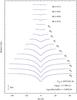 |
Fig. 1 Fit to LTE models. |
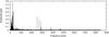 |
Fig. 2 Amplitude spectrum calculated from the K2 data of EPIC 211779126. The dashed horizontal line represents a detection threshold at 0.0167 ppt. |
The spectra were obtained during three different nights only. The measured RV values are comparable to the scatter of the data and do not reveal an obvious binary. From these data we can rule out a close-orbit binary, unless it is seen at an angle perpendicular to the orbital plane. Additionally, the 2MASS near-IR photometry does not show evidence for any IR excess expected from a low-mass main-sequence companion. From the available data, EPIC 211779126 appears to be a single sdB star.
From a fit to local thermodynamical equilibrium (LTE) models (Heber et al. 2000; Edelmann et al. 2003), with S/N ~ 200, we find the following values for the atmospheric parameters: Teff = 28 557(82) K, log g = 5.396(12) dex and log (NHe/NH) = −3.065(24) dex, with the fit shown in Fig. 1. The parameters are consistent, within the errors, with those determined by previous investigators.
3. Photometry
EPIC 211779126 was observed during K2’s Campaign 5. The observations started on April 27 and finished on July 10, 2015. Both short (SC) and long cadence processed data are available, but for this analysis we used only SC data. During K2, the spacecraft is rolling, as a consequence of missing two reaction wheels. To compensate for this roll, as necessary, thrusters are fired every 5.9 h. This means that pointing is maintained by a combination of two reaction wheels and thrusters. This pointing method causes slow drops or spikes in the light curve. The flux variations caused by spacecraft motion are much larger than those from pulsations and must be removed from the data before the final analysis. Even though the raw light curves appear discouraging, the removal of unstable pointing is relatively simple. First, we used standard IRAF tasks (daofind and phot) to pull out fluxes by means of aperture photometry with a 3.5 pixel aperture. Then, we clipped the data at 4σ and de-correlated fluxes in both directions of a target mask. This latter step removed the flux’s positional dependance on the CCD. The resultant light curve was free of the signatures of thruster firings. Finally, we converted fluxes to parts per thousand (ppt) and the data were ready for Fourier analysis.
4. Fourier analysis
We present the amplitude spectrum of EPIC 211779126 in Fig. 2. It is dominated by signal in the low frequency g-mode region, with additional signal at higher p-mode frequencies. The amplitudes are relatively small, below 0.1%, which explains why Østensen et al. (2010) did not detect any flux variations in their observations. The peak profiles are complicated, which is a consequence of variable amplitudes and/or periods. The profiles (shown in Fig. 3) are discussed in subsequent subsections. Since the amplitudes and/or frequencies vary, we prewhitened the data simply in order to look for other small-amplitude peaks near the prewhitened frequencies, and not to derive precise properties. The frequencies listed in Table A.1 should be considered as an approximate location, particularly where closely spaced frequencies occur. Assuming that 2000 μHz distinguishes between p- and g-modes, we found 183 frequencies in total, including 154 in the g-mode region and 29 in the p-mode region. The detection threshold was 0.0167 ppt and was defined as 5σ (Baran et al. 2015b), where σ is the average noise level in the residual amplitude spectrum equaling 0.00334 ppt. We verified the pulsation content against artifacts presented by Baran (2013).
4.1. p-modes
The spectrum in the p-mode region is relatively rich in peaks and we were successful in identifying modal degrees of some of the modes. The frequency distribution resembles that of Balloon 090100001 (Baran et al. 2009). We also found frequencies that are grouped and separated by almost 1000 μHz, with decreasing widths of the gaps and amplitudes as frequency increases. Such groupings are predicted by theoretical models (Charpinet et al. 2000) and indicate consecutive radial overtones.
In the p-mode region, the only tool we have for identifying pulsation degree, ℓ is frequency multiplets. Stellar rotation removes azimuthal degeneracy, creating 2ℓ + 1 peaks for each degree, each separated by the inverse of the orbital period (assuming the Ledoux constant for low-degree p-modes is negligible). Since the rotation period of EPIC 211779126 was unknown, we had to determine it using commonly-spaced frequency multiplets.
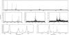 |
Fig. 3 Amplitude spectrum of the p-mode region. Top panel: most of the p-modes. The middle panels are zoomed to show details of the three groups of modes, while the bottom panels zoom in on the two best p-mode multiplets. |
In Fig. 3 we show all the interesting p-mode regions. The top panel includes three groups of frequencies, which are likely separated as consecutive radial overtones. The middle panels show close-ups of those three groups. The left plot centers at three frequencies with the highest amplitudes. In fact, the two lower frequencies look like singlets, while the highest frequencies have some additional signal to the left. These are likely a quintuplet and a triplet with an average splitting of 0.707 μHz which we show in the bottom panels of Fig. 3 and discuss in Sect. 4.3. The center and right middle panels show higher frequencies. The profiles of the peaks in these two regions are very complicated and we did not expect a prewhitening process to work efficiently. These regions resemble the high end of the amplitude spectrum of KIC 10139564 presented by Baran et al. (2012). We checked the superNyquist region and can confirm that these frequencies do not originate from that region. Only the two multiplets near 2900 μHz allow unambiguous mode identifications using frequency multiplets.
4.2. g-modes
The g-mode region has a rich content. The amplitudes are comparable to those of p-modes, with the highest being almost 0.8 ppt. We present the g-mode region up to 2000 μHz in Fig. 4. From the p-mode multiplets, assuming a solid-body rotation, we can estimate rotational splittings for g-mode multiplets to be 0.35 μHz for l = 1 and 0.59 μHz for l = 2. Such splittings should be resolved in our data, as the frequency resolution is equal to 0.23 μHz. Consistent rotational splittings in p- and g-modes are observed in KIC 10139564 (Baran et al. 2012) which means that solid body rotation exists in sdB stars. On the other hand, Foster et al. (2015) showed that KIC 3527751 experiences internal differential rotation, with the core rotating three times slower than the envelope. If the core of EPIC 211779126 rotates more slowly, then g-mode splittings will not agree with our predictions and multiplets could remain unresolved. If the core rotates faster than the envelope then multiplets should easily be resolved. Our observations do not support the latter case.
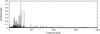 |
Fig. 4 Amplitude spectrum in the g-mode region. |
To verify whether multiplets are present in the g-mode region we used an extra tool to examine the data. When amplitude, phase, and/or frequency variations occur during observations, they are not well accounted for in the integrated amplitude spectrum. As such, we also examined sliding amplitude spectra (time-frequency diagrams) of subsets of the data. We examined amplitude spectra spanning 10, 15, and 20 days of data, stepped in two-day increments. The 20-day subsets are shown as sliding amplitude spectra in the top panels of Figs. 5 and 6 with examples of the individual amplitude spectra in the bottom panels. We used the sliding amplitude spectra to guide which individual amplitude spectra to use for determining the frequency and amplitude. As those data are shorter, the noise is higher, and so rather than list amplitudes in Table A.1, we only list S/N.
Figures 4 and 5 show that we clearly do not detect g-modes with splittings of 0.35 or 0.59 μHz. The implications of this are discussed further in Sect. 4.3.
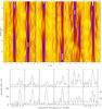 |
Fig. 5 Temporal examination of pulsations. Sliding amplitude spectra (top panels) show the time evolution of pulsations. Time is on the ordinate, relative frequency on the abscissa and color indicates amplitude in σ. White (saturated) pixels indicate amplitudes above 41, 40, 55, 27, 15, and 40σ for central frequencies of 102.55, 112.9, 124.1, 158.2, 166.0, and 179.9 μHz, respectively. Bottom panels: individual amplitude spectra which make up the sliding amplitude spectra on top. Dashed horizontal lines indicate 5σ. Note that the ordinate scale changes between panels, indicated by the position of the 5σ lines. |
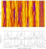 |
Fig. 6 Similar to Fig. 5 but with panels centered at 618.65, 845.5, 1006.0, 158.2, 1142.5, and 2884.2 μHz with color limits of 10.2, 19.7, 5.0, 27, 11.5, and 11.7σ. |
To identify the radial order of pulsation modes, we used an asymptotic relation, which separates consecutive radial overtones in period. The known spacing for sdBV stars is approximately 250 and 150 s, for dipole and quadrupole modes, respectively (Reed et al. 2011). Since the effect of surface cancelation leaves higher detectable amplitudes for l = 1 modes, we started our search with a sequence of dipole modes. The highest-amplitude modes are separated by almost 250 s and we used them as a baseline for our l = 1 sequence. At some frequencies, there are too many modes to assign them all with only one sequence. Initially we tried to complete the l = 1 sequence, but modes which did not match that sequence were checked against the l = 2 sequence. l ≥ 3 modes are not commonly detectable in amplitude spectra and so a l ≥ 3 sequence would not likely be well-populated. As such, we did not seek to identify those modes using asymptotic period spacings. We arbitrarily chose the closest highest-amplitude period to be l = 1 and, where sequences overlapped, the second highest as l = 2. Some times there are other periods with lower amplitudes which could fit one or both sequences and it is possible one of these is the actual l = 1 or 2 mode. However, changing that assignment would not significantly change the period spacings. In Fig. 7 we show the result of our period spacing search.
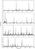 |
Fig. 7 Modal degree assignment. Note that the horizontal axis is in period instead of frequency. |
We found a complete sequence of dipole modes from 2900 to 11 000 s. The sequence contains 31 radial overtones. We also found quite a long, although incomplete, sequence of quadrupole modes from 2400 to 5100 s. We were successful in assigning modal degree and radial order, n, to most of the frequencies in the g-mode region. Pulsations above 500 μHz are not well-separated in period, making our search for 250 or 150 s spacings difficult. Also, asymptotic spacings would not be expected for l ≤ 2 modes in this region as they would not have l ≪ n. On the other hand, if they are high-degree modes, then their radial order could be similar to the ℓ ≤ 2 modes.
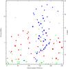 |
Fig. 8 Échelle diagram appropriate for dipole modes (blue dots). All periods are shown with red squares indicating ℓ = 2 modes and green diamonds for unidentified modes. Black outlines indicate trapped modes. |
4.3. Multiplets and period of rotation
Frequency multiplets in EPIC 21179126 are complex and unique for sdBV stars. The two multiplets between 2880 and 2920 μHz (bottom panels of Fig. 3) are the most straightforward to interpret. The splittings in both multiplets are consistent, with four frequencies in the left plot and three in the right. We anticipate that the multiplet in the left plot has an additional fifth component (marked with a dashed vertical line) that is not driven to a detectable amplitude. We assume these multiplets represent rotationally split modes. The splitting equals 0.707 μHz which translates to a rotation period of 16 days. Such a period is shorter than most other sdBV stars observed during the Kepler mission and is comparable to the rotation period of Balloon 090100001 (Baran et al. 2009).
Beyond these two multiplets, it becomes more difficult to interpret. The higher frequencies, as mentioned in Sect. 4.1, are more variable, making their frequencies less secure. This same feature was observed in the p modes of Balloon 090100001 (Baran et al. 2009) and KIC 3527751 (Foster et al. 2015). While we cannot directly assign modes based on their multiplet structure, we find six splittings near those of f161–f168, or an integer multiple, therefore they are consistent.
We find interesting multiplets between 500 and 1202 μHz. Most of the frequencies in this region are part of complex multiplets with spacings near those of the p-mode region. High-degree g-mode frequencies have previously been detected in the lower portion of this region using extended Kepler data sets (Foster et al. 2015; Telting et al. 2014). Within the limits of K2, it is more difficult to determine frequencies, and we rely on sliding amplitude spectra to guide our frequency extraction. Still, we typically only list two or three frequencies, while the region itself may contain more (see Fig. 6). If these are portions of high-degree (ℓ ≥ 4) modes, then the Ledoux constant, Cn,ℓ is small, and the splittings should be roughly equal to those of p-modes, which is what we find. However, we have not previously observed high-degree g-modes above 900 μHz, and so EPIC 21179126’s near-continuous frequency spectrum between the g- and p-mode regions is unique.
We also find a few frequency separations at low frequencies which are clearly within the g-mode range, yet similar to those in the p-mode region. These are much more difficult to interpret. If EPIC 21179126 were a solid-body rotator, as indicated by the >500 μHz splittings, then low-degree (ℓ ≤ 2) modes should have splittings of 0.35 and 0.59 μHz. Such splittings would be resolved in our data set and be easy to detect in the higher-amplitude pulsations, yet we clearly do not detect them (see Figs. 4 and 5). We interpret the g-mode multiplets below 500 μHz to be chance alignments caused by the frequency density of the region or amplitude and/or phase variations (see Fig. 5), which would indicate that the core does not co-rotate with the envelope. There are some multiplet-like peaks (at approximately 8000 and 9600 s in Fig. 4) but the splitting is very small and more likely caused by amplitude and/or phase variations (see Fig. 5). Even if these were caused by rotation, they would indicate a slower rotation for the core.
When we examine the frequency multiplets present in EPIC 21179126, we are presented with a unique situation. The p-mode region shows two characteristic multiplets and several others with consistent splittings, most easily interpretable as stellar rotation with a period of approximately 16 days. The lower g-mode region (below 500 μHz) does not show any obvious multiplets, even though there are high-amplitude peaks that would resolve into multiplets if EPIC 21179126 rotated as a solid body. This region strongly indicates that the core rotates more slowly, leaving rotational multiplets unresolved in this data set. In the upper g-mode region (500–1200 μHz), there are many complex multiplets with splittings commensurate to those in the p-mode region. Frequencies in the lower portion of this region have previously been found to be high-degree g modes in other sdBV stars. These are low-amplitude, complex, frequency/amplitude structures, which are less reliable than the much higher-amplitude low-degree g modes in the lower regions. As such, our best interpretation is that the envelope rotates with a period of approximately 16 days and most likely the core rotates more slowly.
4.4. The échelle diagram
After determining a characteristic period spacing ΔP of approximately 256 s we can generate the échelle diagram by plotting P modulo ΔP versus P. A distinctive ℓ = 1 sequence is produced when plotting with ΔP = 256 s, with the sequence showing a characteristic meandering curve (Fig. 8). The corresponding ℓ = 2 sequence can be found by plotting the same data modulo using the predicted spacing for ℓ = 2, ΔP = 256/ = 148 s (Fig. 9). Note, that the ℓ = 2 sequence shows the same meandering pattern as the ℓ = 1 sequence, only shifted to shorter periods, which corresponds to the asymptotic order n (as indicated on the right-side axes in the figures). These observed échelle diagrams are very similar to those presented by Charpinet et al. (2013, 2014a,b), which confirm the theoretical expectations obtained by using the newest models of sdB stars.
After assigning ℓ to the modes (see Table A.1), we can convert all periods, P, to reduced period, Π, according to  and subsequently compute the differences ΔΠ between consecutive modes. When plotting ΔΠ as a function of Π we obtained the reduced period diagram (Fig. 10).
We used the asymptotic relation to define n values for our modes, and these values are listed in Table 2. We note that there may be a zero-point offset nl between the listed n values and the actual n values of the modes, an offset that we cannot determine without detailed modeling (see e.g., Charpinet et al. 2000). Furthermore, any trapped mode is effectively inserted between the asymptotic radial orders, implying smaller period spacings between subsequent modes in the radial-order range around the trapped mode.
The identification of a trapped mode (for more details see Østensen et al. 2014a) between radial orders n = 20 and 21 is very convincing as it is well-matched in both the ℓ = 1 and ℓ = 2 sequences. The possible trapped mode indicated at approximately n = 14 is much less convincing, because dips in both sequences do not overlap.
5. Summary
We present our discovery and analysis of the sdBV star, EPIC 211779126. The amplitude spectrum shows a very rich content in the low-frequency region with additional signal in the high-frequency region. This makes EPIC 211779126 a rare, richly pulsating hybrid. Its rich, hybrid nature should provide secure constraints over a wider range of stellar properties, since p- and g-modes have information from different parts of a star.
We searched the amplitude spectrum for rotational multiplets and asymptotic period spacings. Both features help with identification of modal degrees and radial orders that are relative to arbitrary zero-point, while the former also determines the rotational period. We found some convincing multiplets among p-mode pulsations whilst we did not find any obvious ones among the g-modes. This observation presents us with an enigma. If a star rotates, we expect to see multiplets in both p- and g-mode regions. We suspect that EPIC 211779126 rotates differentially and that its core rotates slower than its outer envelope. In such a case, we would not see multiplets among low-degree g-modes, because they are unresolved. We estimated the rotational period of the envelope to be 16 days, while we can only suspect that the core rotates slower, such as that of KIC 3527751 (Foster et al. 2015).
Among the g-modes, we found two sequences of dipole and quadrupole overtones. The former is relatively complete, covering over 30 radial orders. We were successful in assigning modal degrees of approximately 50% of the modes up to a frequency of 500 μHz. The completeness of the g-mode sequences allows us to calculate a reduced-period plot. The two overlapping sequences clearly indicate trapped modes, similar to some other sdBV stars (Østensen et al. 2014a; Foster et al. 2015). This feature points to a discontinuity in the stellar chemical profile and is a significant factor in calculating theoretical evolutionary models of sdB stars. We do not assign mode identifications in the intermediate region of 500 to 2000 μHz. Between 500 and 1200 μHz there are several complex multiplets indicative of high-degree modes, but amplitude and/or frequency variations prevent us from obtaining clear identifications.
The p-mode region is separated into approximately three groups. These groups are spaced consistently with consecutive radial overtones in models. In all of the groups we see frequency multiplets with a common spacing which indicates a rotation period of approximately 16 days. However, in only one of these groups do we see a clear triplet and quintuplet, from which we can derive modal degrees. The other groups have more complex natures, which prohibit clear modal degree assignment. Such a feature has been observed in other sdBV stars (Baran et al. 2009; Foster et al. 2015)
Our spectroscopic effort does not show any signature of binarity, therefore we assume that EPIC 211779126 is a single star. The spectroscopic parameters obtained from our new spectra place this star in the log g – Teff diagram in the so-called hybrid region, hence, both types of pulsations in one star is not surprising. However, EPIC 211779126 is a rare sdBV star, as both regions have pulsations driven to similar amplitudes and both regions contain many periodicities.
EPIC 211779126 is an sdBV star that provides important constraints for the evolution of sdB stars. It increases our sample of single sdB stars that likely have their own formation channel. Its pulsation content provides near-complete identification of modal degree and relative radial order which will provide substantial constraints on full asteroseismological and stellar evolution models. The rotation period constraints also provide evidence of possible differential rotation.
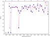 |
Fig. 10 Reduced period diagram. |
Acknowledgments
A.S.B. gratefully acknowledges financial support from the Polish National Science Center under project No. UMO-2011/03/D/ST9/01914. Funding for this research was provided by the National Science Foundation grant #1312869. Any opinions, findings, and conclusions or recommendations expressed in this material are those of the author(s) and do not necessarily reflect the views of the National Science Foundation. Based on observations made with the Nordic Optical Telescope, operated on the island of La Palma by, jointly, Denmark, Finland, Iceland, Norway, and Sweden, in the Spanish Observatorio del Roque de los Muchachos (ORM) of the Instituto de Astrofisica de Canarias operated by the Isaac Newton Group. We thank the anonymous referee for very useful comments that surely improved this manuscript.
References
- Baran, A. S. 2013, Acta Astron., 63, 203 [NASA ADS] [Google Scholar]
- Baran, A. S., & Østensen, R. H. 2013, Acta Astron., 63, 79 [NASA ADS] [Google Scholar]
- Baran, A., Oreiro, R., Pigulski, A., et al. 2009, MNRAS, 392, 1092 [NASA ADS] [CrossRef] [Google Scholar]
- Baran, A. S., Reed, M. D., Stello, D., et al. 2012, MNRAS, 424, 2686 [NASA ADS] [CrossRef] [Google Scholar]
- Baran, A. S., Telting, J. H., Nemeth, P., Bachulski, S., & Krzesinski, J. 2015a, A&A, 573, A52 [NASA ADS] [CrossRef] [EDP Sciences] [Google Scholar]
- Baran, A. S., Koen, C., & Pokrzywka, B. 2015b, MNRAS, 448, 16 [Google Scholar]
- Brassard, P., Fontaine, G., Billères, M., et al. 2001, ApJ, 563, 1013 [CrossRef] [Google Scholar]
- Charpinet, S., Fontaine, G., Brassard, P., et al. 1997, ApJ, 483, 123 [Google Scholar]
- Charpinet, S., Fontaine, G., Brassard, P., & Dorman, B. 2000, ApJS, 131, 223 [Google Scholar]
- Charpinet, S., Fontaine, G., Brassard, P., Green, E., & Chayer, P. 2005a, A&A, 437, 575 [NASA ADS] [CrossRef] [EDP Sciences] [Google Scholar]
- Charpinet, S., Fontaine, G., Brassard, P., et al. 2005b, A&A, 443, 251 [NASA ADS] [CrossRef] [EDP Sciences] [Google Scholar]
- Charpinet, S., Van Grootel, V., Reese, D., et al. 2008, A&A, 489, 377 [NASA ADS] [CrossRef] [EDP Sciences] [Google Scholar]
- Charpinet, S., Van Grootel, V., Fontaine, G., et al. 2011, A&A, 530, L3 [Google Scholar]
- Charpinet, S., Van Grootel, V., Brassard, P., et al. 2013, in Eur. Phys. J. Web Conf. 43, eds. J. Montalbán, A. Noels, & V. Van Grootel, 4005 [Google Scholar]
- Charpinet, S., Van Grootel, V., Brassard, P., & Fontaine, G. 2014a, in Proc. IAU 301, eds. J. Guzik, W. Chaplin, G. Handler, & A. Pigulski, 397 [Google Scholar]
- Charpinet, S., Brassard, P., Van Grootel, V., & Fontaine, G. 2014b, in Meetings on Hot Subdwarf Stars and Related Objects, eds. V. van Grootel, E. Green, G. Fontaine, & S. Charpinet, ASP Conf. Ser., 481, 179 [Google Scholar]
- Edelmann, H., Heber, U., Hagen, H.-J., et al. 2003, A&A, 400, 289 [Google Scholar]
- Fontaine, G., Brassard, P., Charpinet, S., et al. 2012, A&A, 539, A12 [NASA ADS] [CrossRef] [EDP Sciences] [Google Scholar]
- Foster, H., Reed, M. D., Telting, J. H., Østensen, R. H., & Baran, A. S. 2015, ApJ, 805, 94 [NASA ADS] [CrossRef] [Google Scholar]
- Green, E. M., Fontaine, G., Hyde, E. A., Charpinet, S., & Chayer, P. 2006, in 2nd Meeting on Hot Subdwarfs and Related Objects, ed. R. H. Østensen, 15, 167 [Google Scholar]
- Heber, U. 2016, PASP, 128, 2001 [Google Scholar]
- Heber, U., Reid, I. N., & Werner, K. 2000, A&A, 363, 198 [NASA ADS] [Google Scholar]
- Jeffery, C. S., & Ramsay, G. 2014, MNRAS, 442, 61 [Google Scholar]
- Kilkenny, D., Koen, C., O’Donoghue, D., & Stobie, R. S. 1997, MNRAS, 285, 640 [Google Scholar]
- Luo, Y.-P., Németh, P., Liu, C., Deng, L.-C., & Han, Z.-W. 2016, ApJ, 818, 202 [NASA ADS] [CrossRef] [Google Scholar]
- Østensen, R. H., Oreiro, R., Solheim, J.-E., et al. 2010, A&A, 513, L6 [NASA ADS] [CrossRef] [EDP Sciences] [Google Scholar]
- Østensen, R. H., Telting, J. H., Reed, M. D., et al. 2014a, A&A, 569, A15 [NASA ADS] [CrossRef] [EDP Sciences] [Google Scholar]
- Østensen, R. H., Reed, M. D., Baran, A. S., & Telting, J. H. 2014b, A&A, 564, L14 [NASA ADS] [CrossRef] [EDP Sciences] [Google Scholar]
- Randall, S., van Grootel, V., Fontaine, G., Charpinet, S., & Brassard, P. 2009, A&A, 507, 911 [NASA ADS] [CrossRef] [EDP Sciences] [Google Scholar]
- Reed, M. D., Baran, A., Quint, A. C., et al. 2011, MNRAS, 414, 2885 [Google Scholar]
- Reed, M. D., Baran, A. S., Østensen, R. H., et al. 2016, MNRAS, 458, 1417 [NASA ADS] [CrossRef] [Google Scholar]
- Telting, J. H., Østensen, R. H., Baran, A. S., et al. 2012, A&A, 544, A1 [NASA ADS] [CrossRef] [EDP Sciences] [Google Scholar]
- Telting, J. H., Baran, A. S., Németh, P., et al. 2014, A&A, 570, A129 [NASA ADS] [CrossRef] [EDP Sciences] [Google Scholar]
- Van Grootel, V., Charpinet, S., Fontaine, G., & Brassard, P. 2008a, A&A, 483, 875 [NASA ADS] [CrossRef] [EDP Sciences] [Google Scholar]
- Van Grootel, V., Charpinet, S., Fontaine, G., et al. 2008b, A&A, 488, 685 [NASA ADS] [CrossRef] [EDP Sciences] [Google Scholar]
- Van Grootel, V., Charpinet, S., Fontaine, G., Green, E., & Brassard, P. 2010a, A&A, 524, A63 [NASA ADS] [CrossRef] [EDP Sciences] [Google Scholar]
- Van Grootel, V., Charpinet, S., Fontaine, G., et al. 2010b, ApJ, 718, 97 [Google Scholar]
- Vennes, S., Kawka, A., & Nemeth, P. 2011, MNRAS, 410, 2095 [NASA ADS] [Google Scholar]
- Winter, C. 2006, Ph.D. Thesis, Armagh Observatory, The Queen’s University of Belfast [Google Scholar]
Appendix A: Additional table
Frequency list obtained by visual inspection of the sliding amplitude spectra as well as the overall amplitude spectrum of EPIC 211779126.
All Tables
Frequency list obtained by visual inspection of the sliding amplitude spectra as well as the overall amplitude spectrum of EPIC 211779126.
All Figures
|
Fig. 1 Fit to LTE models. |
| In the text | |
|
Fig. 2 Amplitude spectrum calculated from the K2 data of EPIC 211779126. The dashed horizontal line represents a detection threshold at 0.0167 ppt. |
| In the text | |
|
Fig. 3 Amplitude spectrum of the p-mode region. Top panel: most of the p-modes. The middle panels are zoomed to show details of the three groups of modes, while the bottom panels zoom in on the two best p-mode multiplets. |
| In the text | |
|
Fig. 4 Amplitude spectrum in the g-mode region. |
| In the text | |
|
Fig. 5 Temporal examination of pulsations. Sliding amplitude spectra (top panels) show the time evolution of pulsations. Time is on the ordinate, relative frequency on the abscissa and color indicates amplitude in σ. White (saturated) pixels indicate amplitudes above 41, 40, 55, 27, 15, and 40σ for central frequencies of 102.55, 112.9, 124.1, 158.2, 166.0, and 179.9 μHz, respectively. Bottom panels: individual amplitude spectra which make up the sliding amplitude spectra on top. Dashed horizontal lines indicate 5σ. Note that the ordinate scale changes between panels, indicated by the position of the 5σ lines. |
| In the text | |
|
Fig. 6 Similar to Fig. 5 but with panels centered at 618.65, 845.5, 1006.0, 158.2, 1142.5, and 2884.2 μHz with color limits of 10.2, 19.7, 5.0, 27, 11.5, and 11.7σ. |
| In the text | |
|
Fig. 7 Modal degree assignment. Note that the horizontal axis is in period instead of frequency. |
| In the text | |
|
Fig. 8 Échelle diagram appropriate for dipole modes (blue dots). All periods are shown with red squares indicating ℓ = 2 modes and green diamonds for unidentified modes. Black outlines indicate trapped modes. |
| In the text | |
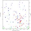 |
Fig. 9 Same as in Fig. 8 for quadrupole modes. |
| In the text | |
|
Fig. 10 Reduced period diagram. |
| In the text | |
Current usage metrics show cumulative count of Article Views (full-text article views including HTML views, PDF and ePub downloads, according to the available data) and Abstracts Views on Vision4Press platform.
Data correspond to usage on the plateform after 2015. The current usage metrics is available 48-96 hours after online publication and is updated daily on week days.
Initial download of the metrics may take a while.