| Issue |
A&A
Volume 597, January 2017
|
|
|---|---|---|
| Article Number | A119 | |
| Number of page(s) | 12 | |
| Section | Interstellar and circumstellar matter | |
| DOI | https://doi.org/10.1051/0004-6361/201629493 | |
| Published online | 12 January 2017 | |
Anatomy of the internal bow shocks in the IRAS 04166+2706 protostellar jet
1 Observatorio Astronómico Nacional (IGN), Alfonso XII 3, 28014 Madrid, Spain
e-mail: This email address is being protected from spambots. You need JavaScript enabled to view it.
2 Academia Sinica, Institute of Astrophysics (ASIAA), and Theoretical Institute for Advanced Research in Astrophysics (TIARA), Academia Sinica, 11F of Astronomy-Mathematics Building, AS/NTU, No.1, Sec. 4, Roosevelt Rd, Taipei 10617, Taiwan
3 National Research Council of Canada, Herzberg Astronomy & Astrophysics, 5071 West Saanich Road, Victoria, BC, V9E 2E7, Canada
4 Department of Physics and Astronomy, University of Victoria, Victoria, BC V8P 1A1, Canada
5 Harvard-Smithsonian Center for Astrophysics, 60 Garden Street, Cambridge, MA 02138, USA
6 Instituto de Radioastronomía Milimétrica (IRAM), Avenida Divina Pastora 7, Núcleo Central, 18012 Granada, Spain
7 Graduate Institute of Astronomy and Astrophysics, National Taiwan University, No. 1, Sec. 4, Roosevelt Road, Taipei 10617, Taiwan
Received: 5 August 2016
Accepted: 27 September 2016
Abstract
Context. Highly collimated jets and wide-angle outflows are two related components of the mass-ejection activity associated with stellar birth. Despite decades of research, the relation between these two components remains poorly understood.
Aims. We study the relation between the jet and the outflow in the IRAS 04166+2706 protostar. This Taurus protostar drives a molecular jet that contains multiple emission peaks symmetrically located from the central source. The protostar also drives a wide-angle outflow consisting of two conical shells.
Methods. We have used the Atacama Large Millimeter/submillimeter Array (ALMA) interferometer to observe two fields along the IRAS 04166+2706 jet. The fields were centered on a pair of emission peaks that correspond to the same ejection event. The observations were carried out in CO(2–1), SiO(5–4), and SO(JN = 65–54).
Results. Both ALMA fields present spatial distributions that are approximately elliptical and have their minor axes aligned with the jet direction. As the velocity increases, the emission in each field moves gradually across the elliptical region. This systematic pattern indicates that the emitting gas in each field lies in a disk-like structure that is perpendicular to the jet axis and whose gas is expanding away from the jet. A small degree of curvature in the first-moment maps indicates that the disks are slightly curved in the manner expected for bow shocks moving away from the IRAS source. A simple geometrical model confirms that this scenario fits the main emission features.
Conclusions. The emission peaks in the IRAS 04166+2706 jet likely represent internal bow shocks where material is being ejected laterally away from the jet axis. While the linear momentum of the ejected gas is dominated by the component in the jet direction, the sideways component is not negligible, and can potentially affect the distribution of gas in the surrounding outflow and core.
Key words: stars: formation / ISM: individual objects: IRAS 04166+2706 / ISM: jets and outflows / ISM: molecules / radio lines: ISM
© ESO, 2017
1. Introduction
Highly collimated jets and wide-angle molecular outflows are common signatures of stellar birth. They are thought to represent two aspects of the same mass-loss phenomenon and to arise from the need of a protostar to release angular momentum as it contracts. Despite decades of study, however, the exact relation between these two forms of ejection is still a matter of debate (Frank et al. 2014; Arce et al. 2007). One popular view is that the jets are the denser, inner parts of wide-angle protostellar winds, and that these wider winds are the true accelerating agents of the large-scale outflows (Shu et al. 2000; Shang et al. 2006). A popular alternative defends the view that the jets are the sole driving agents of the outflows, and that there is no need to invoke an unseen wide-angle component to explain the less-collimated appearance of the molecular flows. According to this view, the action of the narrow jets can be widened by several mechanisms, including jet precession or wandering, entrainment, and the lateral ejection of material in internal jet shocks (Masson & Chernin 1993; Stahler 1994; Raga & Cabrit 1993).
While observations of individual outflows often support either the wide-angle wind or jet-only picture, systematic studies of outflow morphology and kinematics have shown that no single model can explain the variety of observations (Lee et al. 2000). Compounding this problem is the rarity of systems where both the highly collimated jet and the molecular outflow can be studied simultaneously. This limitation partly results from an observational bias, since the detection of a jet, because of its atomic composition, needs to be carried out at optical or infrared wavelengths, which favors objects with little obscuration. However, the detection of a molecular outflow is achieved in the radio, and therefore requires a highly embedded system (Chernin & Masson 1995).
Fortunately, observations have slowly revealed that there is a small group of protostars where both the jet and molecular outflow can be studied simultaneously. These protostars, probably due to their extreme youth, have highly collimated jets that are molecular instead of atomic, and therefore can be observed with the same molecular tracers as those used to study the wider angle outflows. Examples of these young protostars are L1448-mm and IRAS 04166+2706 (IRAS 04166 hereafter). These systems present molecular spectra with characteristic secondary components of extremely high velocity (EHV) gas that are distinctly separated from the standard outflow wings (Bachiller et al. 1990; Tafalla et al. 2004, 2010). When the EHV components are observed with high angular resolution, they are found to trace highly collimated molecular jets that travel inside conical cavities whose walls represent the lower velocity, wide-angle outflows (Guilloteau et al. 1992; Bachiller et al. 1995; Santiago-García et al. 2009; Hirano et al. 2010; Wang et al. 2014). Although L1448-mm and IRAS 04166 represent the finest examples of molecular jets, they are not the only examples. Systems like HH 211 and HH 212 also present highly collimated molecular jets, but their low inclination angle with respect to the plane of the sky hinders the detection of clearly detached EHV features in the spectra (Gueth & Guilloteau 1999; Palau et al. 2006; Lee et al. 2007; Codella et al. 2014; Lee et al. 2015).
In this paper we present Atacama Large Millimeter/submillimeter Array (ALMA) observations of the molecular jet driven by IRAS 04166. This protostar is a 0.4 L⊙ class 0 source in the Taurus molecular cloud at an estimated distance of 140 pc (Elias 1978; Torres et al. 2007). The outflow of this protostar presents a remarkable jet-plus-cavity morphology. Interferometric observations by Santiago-García et al. (2009) and Wang et al. (2014) (SG09 and W14 hereafter) have resolved the IRAS 04166 jet into a collection of discrete emission peaks that are located symmetrically with respect to the IRAS position, and which likely correspond to a number of pulsation events in the history of the jet ejection. Position-velocity diagrams along the jet axis made by these authors reveal that each emission peak has an internal linear velocity gradient where the gas that appears closer to the source moves faster than the gas that appears further away. This type of velocity gradient matches the prediction from models of pulsating jets (e.g., Wilson 1984; Raga et al. 1990; Stone & Norman 1993), which show that variability in the velocity of ejection at the jet base creates a series of internal shocks where rapidly moving jet material overtakes slower gas launched previously. When these shocks occur, the gas inside the jet is ejected sideways and the projection of this motion along the line of sight produces a characteristic saw-toothed pattern (e.g., Fig. 16 in Stone & Norman 1993).
Unfortunately, the observations of the IRAS 04166 jet by SG09 and W14 lacked the necessary sensitivity to study the 2D velocity field of the gas in the EHV emission peaks, and the interpretation of the lateral ejection motions had to rely on the analysis of 1D position-velocity diagrams. The recent online availability of ALMA, with its significant increase in sensitivity and image quality, has now made it possible to study the 2D velocity structure of the relatively weak jet emission in detail. In this paper, we present ALMA observations of the IRAS 04166 jet aimed to determine the full velocity field of two selected EHV emission peaks. By using the ALMA interferometer, and by concentrating on only two jet positions, these observations were designed to achieve high enough sensitivity to study the internal motions of the EHV gas. As shown below, the new observations not only confirm the previous interpretation of the kinematics of the EHV gas, but provide a detailed picture of how the gas is laterally ejected in this remarkable molecular jet.
2. Observations
We used ALMA to observe the two target fields indicated with circles in Fig. 1. These fields are located at offsets ( ,
,  ) and (
 ,
,  ) with respect to the position of IRAS 04166 at
  δ(J2000) = + 27°13′36′′ (SG09). They were observed jointly during two 1.3-h ALMA scheduling blocks in December 2014, as part of Early Science Cycle 1 project 2012.1.00304.S (PI Yu-Nung Su). The Band 6 receivers were tuned to a frequency of 230.5 GHz, to observe simultaneously CO(2−1), SiO(J = 5–4), and SO(JN = 65–54). The correlator was configured to provide a velocity resolution of approximately 0.32 km s-1. The telescope array was in its C32-2 configuration and the baselines between its 12 m antennas ranged approximately between 15 and 330 m. Because of shadowing limitations caused by the low declination of the source, no observations with the compact Morita Array were made for this project.
The ALMA observations consisted of alternating pointings on the two target fields interspersed with observations of J0510+1800 for phase calibration. The same continuum source was used for flux calibration, and J0423-0120 was used to calibrate the bandpass. The resulting visibility data were reduced using the observatory pipeline in CASA version 4.3.1 (McMullin et al. 2007), which was used for calibration, image synthesis, and preliminary cleaning. Imaging was carried out using briggs weighting with a robust parameter of 0.5, and resulted in a synthesized beam of  for the higher frequency CO(2–1) line (230.5 GHz) and
  for the lowest frequency SiO(5–4) line (217.1 GHz). Final cleaning of the maps was carried out using the MAPPING program of the GILDAS software1, although no significant differences were found between the cleaning results from CASA and MAPPING. The typical rms noise level in the maps is 2.5 mJy beam-1 (=35 mK) per 0.5 km s-1 channel.
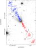 |
Fig. 1 Large-scale image of the IRAS 04166 jet with circles representing the ALMA target positions. The color scale and contours represent the CO(2–1) EHV emission observed by SG09 with the IRAM PdBI, and the background grayscale is an archival Spitzer/IRAC1 image. The two 25′′ diameter circles represent the fields of view of the ALMA antennas. The B5, B6, and R6 labels indicate the emission peaks identified by SG09 and further studied in this paper. |
3. Results
Figure 1 shows, with circles, the location of the two ALMA fields on a colored image of the EHV CO(2–1) emission obtained with the IRAM PdBI. The fields were chosen to cover a pair of emission peaks labeled B6 and R6 in the SG09 notation, and these seem to have resulted from an ejection event that occurred about 900 yr ago. They were selected as ALMA targets because they are well separated from the other emission peaks within the jet, and because their size matches the primary beam of the 12 m ALMA antennas (25′′FWHM). In this paper, we refer to these as the “northern” and “southern” fields, and unless indicated, we color code the first one in blue and the second one in red following the color of the outflow lobe to which they belong.
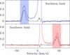 |
Fig. 2 Comparison between the IRAM 30 m single dish spectra from T04 (blue and red histograms) and ALMA spectra synthesized for the same positions and angular resolution (11′′). The color vertical bands indicate the location of the blue and red EHV regimes. There is a good agreement between the 30 m and ALMA spectra inside the EHV ranges, which is indicative of only minor missing flux. IRAM 30 m data in Tmb scale and ALMA data in TB scale. |
The ALMA observations did not include the compact array, and as a result, they may be missing flux from the largest spatial scales. For this reason, we start our analysis by comparing the ALMA observations with single-dish data, which contain all the flux and thus provide a reliable reference. We use the CO(2–1) line because it is the brightest and most extended line in the ALMA observations and, therefore, the most sensitive line to the missing flux problem. As for single dish data, we use the spectra from Tafalla et al. (2004, T04 hereafter), who mapped the CO(2–1) emission of the IRAS 04166 outflow with the IRAM 30 m single-dish telescope. From these data we chose the two positions closest to each of the ALMA fields, and we compared these positions with spectra synthesized from the ALMA data assuming the same position and angular resolution as the 30 m observations (11′′FWHM). Figure 2 shows the ALMA-30 m comparison using colored histograms for the single-dish data and black histograms for the synthesized ALMA data.
As can be seen, the ALMA spectra match well the single-dish data for velocities inside the EHV regime (color-shaded bands), where the intensity agreement between the two spectra is within about 30% at the line peak. This match implies that the ALMA observations recover most of the emission inside the EHV regime, and that the lack of compact array data does not significantly affect the observations of the EHV gas.
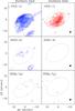 |
Fig. 3 Maps of the integrated EHV emission in the two ALMA target fields for the three main transitions in the setup: CO(2–1) (upper row of panels), SiO(5–4) (middle row), and SO(JN = 65–54) (bottom row). First contour and contour interval are 1.0 K km s-1 in the CO(2–1) maps and 0.5 K km s-1 in the SiO and SO maps. The dashed ellipses delineate the approximate boundaries of the CO emission. The small filled ellipses in the maps of the southern field indicate the synthesized beam for each transition. |
In contrast with the EHV regime, the emission from the low-velocity outflow is mostly missing in the ALMA observations (see velocities near the systemic value of 6.7 km s-1). This loss is caused by the very extended nature of this emission, whose size exceeds the ALMA primary beam, and which can only be mapped using mosaicking techniques. For this reason, we do not study the slow outflow component and our analysis is restricted to the EHV regime.
3.1. Integrated intensity maps
Figure 3 shows maps of the emission integrated over the EHV regime for the three lines of our setup: CO(2–1), SiO(5–4), and SO(JN = 65–54). The EHV regime is defined as the 20 km s-1-wide velocity range that is centered on | V0 ± 37.5 km s-1 |, where V0 is the LSR velocity of the ambient cloud (6.7 km s-1, T04), and the plus and minus signs correspond to the red and blue shifted parts of the EHV regime, respectively.
As can be seen in the top panels of Fig. 3, CO is detected in both target fields with high signal-to-noise ratios. In each target, most of the CO emission lies inside an approximately elliptical region that we indicated in the figure with dashed lines, and which is further discussed below. The northern field presents additional CO emission to the southwest, outside the ellipse, and close to the edge of the ALMA field of view. This extra emission seems to correspond to the nearby B5 EHV emission peak, which according to the estimate by SG09, lies  SW of B6 (Fig. 1). Since we have not corrected the maps in Fig. 3 for the attenuation of the primary beam of the antennas (to avoid amplifying noise near the edges), the emission from the B5 peak is significantly weakened and distorted in the image.
In contrast with CO(2–1), the SiO(5–4) emission is barely detected inside the elliptical regions (Fig. 3, middle panels). In the northern field, the off-center B5 peak is clearly detected, and its emission overshadows the emission from the target B6 peak. A brighter B5 emission peak is expected from the data of SG09, who mapped SiO(2–1) together with CO(2–1), and found that the SiO emission from both B6 and R6 is much weaker than the emission from the inner jet peaks. Although the maps of Fig. 3 suggest that there is negligible SiO(5–4) emission in the elliptical regions, this is somewhat exaggerated by integrating the signal over the 20 km s-1-wide EHV regime. As we see in the next section, the EHV regime has a large-scale velocity gradient and the intrinsic velocity width of the emission at any position is significantly lower than the full width of the EHV range. As a result, integrating the emission over the full 20 km s-1-wide EHV regime dilutes the signal and decreases the sensitivity to weak features. Narrower channel maps show some SiO emission inside the elliptical regions of both fields, but the behavior of this emission seems so similar to that of the much brighter CO (presented in the next section) that its analysis adds very little to the study of our target fields (see Appendix A for channel maps of the SiO emission).
The last transition in our setup, SO(JN = 65–54), was not detected inside the elliptical regions of either ALMA field, even when using narrow channel maps (Fig. 3, bottom panels). The B5 peak was marginally detected inside a narrow velocity range, but its signal is strongly attenuated by the ALMA primary beam. Because of its weak signal, the SO emission is not further discussed here.
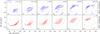 |
Fig. 4 Channel maps of CO(2–1) emission for the northern (top, color-coded blue) and southern (bottom, color-coded red) ALMA fields. For each field, the maps cover the 20 km s-1-wide range shaded with color in Fig. 2. The velocity range of each map, after correction for a jet velocity of 37.5 km s-1, is indicated in the top row in units of km s-1. First contour and step are 20% of the map emission peak, which is indicated for each panel in the bottom left corner in units of K km s-1. The dashed ellipses delineate the approximate boundary of the emission. The emission from SW to NE is gradually displaced as the velocity increases. |
3.2. Velocity structure: Evidence of expanding gas disks
The spectra in Fig. 2 show that the red and blue EHV components are symmetrically offset in velocity with respect to the ambient cloud (at VLSR = 6.7 km s-1). We estimated the value of this offset using a a Gaussian fit to the spectra, deriving a velocity of 37.5 km s-1 for both the blue and red EHV components. This offset velocity likely represents the mean radial velocity of the IRAS 04166 jet, and as a first step in our analysis, we corrected the EHV emission in each ALMA field by this value. In this way, our study concentrates on the internal motions of the EHV gas and measures them in the local rest frame of the jet.
Having set the mean gas velocity to zero in each field, we now divide the 20 km s-1-wide EHV regime into multiple velocity channels. Figure 4 shows the result for the case of six equally spaced channels of 3.33 km s-1 width, although other width choices produce similar maps. As the figure shows, the two ALMA fields present very similar velocity patterns. The emission at the lowest (bluest) velocities lies toward the southwest boundary of the dashed ellipse, and as the velocity increases, the emission moves gradually from SW to NE sweeping the full elliptical region. Finally, the reddest EHV emission lies near the NE boundary of the ellipse and appears approximately mirror-symmetric with respect to the extremely blue emission. This systematic SW-to-NE shift of the emission with increasing velocity is not only seen in the emission inside the two ellipses. It can also be seen in the off-center B5 peak of the northern field, although the pattern here is less prominent than in B6 and R6 owing to the strong effect of the primary-beam attenuation.
The systematic shift of the emission as a function of velocity matches the sense of the velocity gradients found by SG09 and W14 in their PV diagrams along the jet axis. These PV gradients show that in each EHV peak, the absolute value of the radial velocity decreases with distance to the source. As Fig. 4 shows, this is the same sense of the velocity gradient found in the channel maps: the reddest gas of the red (southern) field is found at positions closer to the central source (toward the NE), and the bluest gas in the blue (northern) field is also found toward positions closer to the source (in this case toward the SW). The gas motions seen in Fig. 4 therefore represent the velocity structure underlying the gradients previously seen in the PV diagrams.
The velocity gradients in the PV diagrams were interpreted by SG09 and W14 as arising from the sideways ejection of gas in a series of internal jet shocks. This interpretation was based on a comparison of the observed PV diagrams with synthetic diagrams predicted by numerical models of pulsating jets, such as those of (Stone & Norman 1993; see also Völker et al. 1999; and Moraghan et al. 2016). The high level of detail provided by the new ALMA images allows us now to further investigate the lateral ejection interpretation by studying the detailed 2D distribution of the gas velocity field. To do this, we first characterize the elliptical regions that bound the EHV emission in each ALMA field. We use for this the maps of extreme red- and blueshifted velocity in Fig. 4 because they seem to best constrain the curvature of the ellipses. For the northern field, we estimate an ellipse size of about 20′′ × 12′′ (major times minor axis), while for the southern field we estimate a slightly larger size of 22′′ × 14′′.
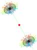 |
Fig. 5 Schematic geometry of the emitting gas. The filled red circle indicates the position of IRAS 04166, and the green line is the direction of propagation of the jet. Each emitting region is represented by a tilted disk of gas that expands perpendicular to the jet axis, and whose velocity vectors have been color coded according to their Doppler shift. This schematic geometry simultaneously reproduces the elliptical shape of the emission and the systematic velocity pattern. (To improve visibility, the size of the disks has been exaggerated in proportion to their distance from the central source.) |
The final parameter needed to characterize the elliptical regions is the position angle (PA). For both ALMA fields, we estimate a value of about − 60°, measured clockwise from north according to the standard convention. This PA value indicates that the minor axis of each ellipse is approximately parallel to the direction of the IRAS 04166 jet, which was determined as  by SG09 from a fit to the emission centroids of all the EHV peaks in the outflow. Such a coincidence between the ellipse minor axis and the direction of the jet strongly suggests that the elliptical shape of the regions is the result of a projection effect and that the true distribution of the gas is in circular disks that are perpendicular to the jet axis. This geometry is illustrated in Fig. 5, where the gas in the two ALMA fields has been represented by two disks of expanding gas. As can be seen, the circular disks are foreshortened into ellipses that have their minor axes parallel to the direction of the jet. In addition, the expansion velocity field of the gas creates a pattern of velocities in which the blueshifted material occupies the SW section of the disk and the redshifted material occupies the NE section. This pattern matches the behavior of the velocity field seen in the channel maps of Fig. 4.
If the elliptical shape of the emission in each ALMA field results from the foreshortening of a circular gas disk, the aspect ratio of the ellipse is an indicator of the inclination angle of the disk with respect to the plane of the sky. From this angle, we can estimate the inclination angle of the jet. As we have seen, the two ALMA fields are fitted with ellipses of very similar aspect ratio, 6/10 and 7/11, and these ratios correspond to jet inclination angles of  and
and  . These values are very similar, especially considering our simple fitting method, so we average them as 52°, and assume a probable uncertainty of less than 10%. With this angle we can deproject the radial jet velocity derived from our Gaussian fit to the EHV emission (37.5 km s-1) and obtain a true jet velocity of about 61 km s-1, again with an uncertainty of about 10%.
3.3. Asymmetry at high velocities: evidence of curvature
So far we have stressed the similarities between the emission in the northern and southern ALMA fields in terms of velocity offset from the ambient cloud, elliptical shape, and velocity pattern. These similarities are indeed the dominant feature of the emission. A close inspection of the data, however, also reveals slight but systematic differences between the emission from the two ALMA fields. One indication of these differences comes from comparing the emission at the most extreme velocities; Fig. 6 shows together the emission in the reddest and bluest 5 km s-1 of the EHV range (top panels). As expected, in both fields the blue emission lies toward the SW and the red emission lies toward the NE. This blue-red symmetry, however, is not perfect. In the northern field, the redshifted emission is significantly narrower and more curved than the blueshifted emission. In the southern field, the asymmetry is reversed: the blueshifted emission is the one that is narrow and curved, while the redshifted emission is wider and rounder.
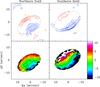 |
Fig. 6 Evidence of curvature in the CO(2–1) emitting regions. Top panels: comparison between the CO emission in the reddest and bluest 5 km s-1 intervals of the EHV range for each ALMA field. First contour and contour interval are 0.5 K km s-1. Bottom panels: first moment maps of the CO(2–1) emission. As in Fig. 4, the velocity scale has been centered on zero by correcting for the source and jet velocities. Data outside the elliptical regions have been masked out as a result of their low signal-to-noise ratio. The wedge to the right shows the scale in km s-1. |
The asymmetry seen at extreme velocities is part of a global pattern that also occurs at intermediate velocities. This is illustrated in the bottom panels of Fig. 6 using maps of the first moment (velocity centroid) of the CO(2–1) emission. The maps show the expected layered distribution that has the blue emission toward the SW and the red emission toward the NE. In addition, the maps show that in each field, the iso-velocity contours are slightly curved and the sense of curvature is opposite in the two fields. In the northern field, the contours curve slightly away from the NE (red edge), while in the southern field, the contours curve away from the SW (blue edge).
The curvature of the first-moment maps in Fig. 6 implies that the expanding gas disks responsible for the emission in each ALMA field are not perfectly flat. They must be slightly curved, or at least their velocity field must present a small degree of curvature. To reproduce the first-moment maps, the curvature must be such that the edge of each disk curves back toward the central IRAS source. This sense of curvature again matches the prediction from numerical models of lateral expansion of gas in an internal jet shock (e.g., Hartigan et al. 1987), which show that the material ejected from the jet curves back because it is slowed down by its interaction with lower velocity gas outside the jet beam. Numerous observations of optical and IR jets show this type of curvature, both at the leading end of the jet and at the internal shocks, likely caused by jet pulsations (e.g., Devine et al. 1997; Zinnecker et al. 1998; Reipurth et al. 2002).
To summarize, the new ALMA observations support the previous interpretation of the EHV emission as arising from gas that has been laterally ejected in a series of jet shocks (SG09 and W14). In addition, the new data provide a detailed picture of the distribution of gas both in space and velocity, thanks to the significant increase in sensitivity afforded by ALMA. In the next section we present a geometrical model aimed at taking advantage of this new sensitivity to further constrain the properties and kinematics of the EHV gas.
4. A geometrical model of the EHV gas
The goal of our model is to reproduce the behavior of the CO emission in the two ALMA fields by assuming that it arises from laterally-expanding material in jet bow shocks. Since the emission from the two ALMA fields looks similar in the velocity maps (Fig. 4) and moment maps (Fig. 6), we assume that the two emitting regions have the same internal structure, and that they only differ in their relative orientation with respect to the central source. By doing this, our model does not attempt to fit the individual details of each ALMA field, but fits the common features of their emission.
 |
Fig. 7 Schematic view of the shell used to model the emission in the southern ALMA field (the northern model is just the reflection image with respect to central source). As in Fig. 5, the green line represents the jet axis and the velocity vectors have been color coded according to their Doppler shift. |
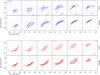 |
Fig. 8 Comparison between observed velocity maps and results from a geometrical model for both the northern (top and blue) and southern (bottom and red) ALMA fields. Both fields have been modeled assuming the same physical conditions but opposite orientation, as expected for two bow shocks moving away from the central IRAS source. Panel velocities, dashed ellipses, and contour levels as in Fig. 4. |
We start our modeling by assuming that the emitting gas is distributed in a shell of parabolic walls, and that the gas expands outward moving parallel to the walls. This geometry is illustrated in Fig. 7 for the southern field and is motivated by the analytic shock models of Hartigan et al. (1987), who found that bow shocks tend to be parabolic in the vicinity of the jet axis. To reproduce our observations, the curvature of the parabola must be very mild (described as z = 0.02r2), and the shell must be truncated when its outer cylindrical radius r reaches a size of 11′′ to match the observed emission size. Our model also assumes that the shell has a thickness of  . This choice is not very critical, since the emission is optically thin and depends only on the column density. Any other choice of the shell thickness can be compensated with a change in the gas density.
We also assume that the gas is isothermal. The single dish observations of CO(1–0) and CO(2–1) by T04 indicate gas temperatures between 7 and 20 K in the different EHV peaks, with a tendency for the colder peaks to be found further away from the IRAS source. Following this trend, we assume that the gas in the shells has a constant temperature of 10 K. We also assume a standard CO abundance of 8.5 × 10⁻⁵ (Frerking et al. 1982).
Once we assume the physical conditions of the gas, we calculate the expected CO emission using a modified version of the ray-tracing program presented in Tafalla et al. (1997). This program integrates the equation of radiative transfer over a grid of positions assuming LTE conditions and taking the gas velocity field into account. We explored a variety of velocity and density laws to fit the data. To fit the velocity maps of Fig. 4, which show that the emission gradually sweeps the elliptical regions and forms a series of narrow bands approximately parallel to the major axis, a constant velocity model does a poor job (Appendix B), and we need to use a velocity field that increases in magnitude with distance from shell center. After some trial and error, we found a best fit using a linear velocity field where the gas expansion increases gradually from 0 to 13 km s-1 at the shell edge.
The gas density law is less well constrained than the velocity, since it depends on our assumption of the shell thickness, and also because the maps of integrated emission do not show a systematic pattern but significant differences between the two ALMA fields (Fig. 3). To reproduce the common gradual decrease of intensity toward the emission edges, we used an inverse square-root density law in the outer half of the shells, and to avoid creating a deep hole at the center, we assumed that the inner half of the shell has a constant density of a 0.8 × 104 cm-3. While this choice may not be unique, it seems to capture the general distribution of mass inside the shells.
Figures 8 and 9 compare the results of our geometrical model with the velocity maps, integrated maps, and first-moment maps of the two ALMA fields. Despite its simplicity, the model reproduces well the main features of the CO emission, especially its elliptical distribution, gradual displacement from SW to NE as a function of velocity, and opposite sense of curvature in the first-moment maps. These characteristics arise from the disk-like distribution of the emitting gas and from its expansion velocity field, and constitute the best-constrained properties of the EHV gas. Their success in modeling the data provide a further confirmation that the EHV emission arises from the internal bow shocks of a pulsating jet.
While the geometrical model fits the data well, the agreement is not perfect. Figure 8 shows that the model emission is significantly more concentrated than observed with ALMA, an effect that is especially noticeable in the maps of intermediate velocities. This discrepancy probably results from our simplified velocity field, which assumes that the gas moves along the shell with no shear and no internal velocity dispersion. This is of course an extreme approximation, since the gas must have additional motions resulting from the dissipation of the supersonic jet velocity in the internal shock. Such complex turbulent motions are indeed seen in numerical simulations of jet shocks, and arise from a number of instabilities (Blondin et al. 1990; Stone & Norman 1993). Adding these motions, likely broadens the emission in the channel maps by increasing the number of shell points that contribute to any given map.
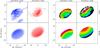 |
Fig. 9 Comparison between maps of integrated intensity (left) and iso-velocity (right) from ALMA observations and the geometrical model presented in the text. For each comparison, the top panels represent the ALMA observations and the bottom panels represent the model. Each comparison uses the same velocity interval and contour levels as in Fig. 3 (integrated maps) and Fig. 8 (iso-velocity maps). |
Despite the above limitation, it seems clear from the model that the kinematics of the CO-emitting gas is dominated by the motions of lateral expansion along the shells. We can therefore use the model fit to constrain the main properties of these motions. An important constraint from the model is the need for the gas velocity to increase in magnitude with distance from the jet axis (Appendix B). This linear velocity gradient could arise from different physical processes. One possibility is that the strength of the jet shock has decreased systematically with time, and that the linear velocity gradient reflects this gradual shock weakening. Both numerical and analytic models of pulsating jets with sinusoidal velocity oscillations show that the strength of the shock is highest at early times, since the original sinusoidal velocity oscillation quickly steepens into a saw-toothed profile that makes the fastest jet gas encounter the slowest gas from the previous cycle, producing the strongest possible shock (Kofman & Raga 1992; Stone & Norman 1993; Smith et al. 1997; Suttner et al. 1997). As time progresses, the relative velocity between the incoming and trailing parts of the jet decreases, and so does the strength of the shock. This decrease is approximately linear, as shown by the analytic model of Kofman & Raga (1992, see their Fig. 2).
An alternative interpretation of the linear velocity gradient is that it is the result of a single shock event that generated gas moving at multiple expansion velocities. In this case, the expanding material would naturally sort itself spatially because each gas parcel would move away from the jet axis proportionally to its expansion velocity. To test the consistency of this interpretation, we estimate the time since the shock event took place by dividing the maximum displacement of the gas from the jet axis (≈11′′) by the largest estimated gas velocity (≈13 km s-1). The result is approximately 550 yr, which is lower than the estimated travel time of the jet gas from the protostar (≈900 yr). This means that an explosive event could have occurred during the flight time of the jet material and, therefore, that the interpretation as a single internal shock event is consistent with the rest of jet properties.
While the origin of the linear velocity gradient is unclear, the pattern occurs in both ALMA fields and is hinted in the off-center B5 peak of the northern field, so it seems to represent a robust characteristic of the EHV emission. Further ALMA observations of the inner EHV peaks along the jet, together with more detailed numerical models of the internal shocks in pulsating jets, are clearly needed to understand this effect.
5. Implications for outflow evolution
The lateral ejection of material in the IRAS 04166 jet has potential consequences for the evolution of both the outflow and its surrounding dense core. To evaluate these consequences, we now use the physical parameters of the ejected gas that we have estimated with the geometrical model. As a first step, we integrate the model density profile of the shell to estimate the amount of mass in each EHV peak. For simplicity, we ignore the slight curvature of the shell and we treat the emitting region as a flat disk of thickness, 11′′ radius, and the density profile described in the previous section. In this way, we derive a shell mass of 8.6 × 10⁻⁵M⊙, which applies to each ALMA field because by construction we have fitted them using the same model. This value is in good agreement with the mass estimates for the B6 and R6 peaks made by SG09 by direct integration of the CO(2–1) intensity, assuming optically thin conditions, which were 8.8 × 10⁻⁵ and 5.9 × 10⁻⁵M⊙, respectively. The agreement between the two estimates is not surprising, since they both make use of CO(2–1) observations of consistent intensity and assume similar excitation conditions. Still, it provides a further test that our simple geometrical reproduces the main properties of the observations.
Using the mass estimate, we calculate the forward momentum in the EHV shell. This is an important outflow parameter, since the momentum is a conserved quantity in contrast with the kinetic energy, which is partly radiated away in shocks. We again assume that the shell is a flat disk, ignoring the small curvature effect. We do this not only because the curvature is very small, but also because bow-shock models show that the curvature is caused by the transfer of momentum from the shell to the surrounding gas in the jet “shroud” (Masson & Chernin 1993); our estimate refers to the momentum originally available in the EHV gas. Since we have estimated that the shell moves in the jet direction with a bulk deprojected velocity of 61 km s-1 (Sect. 3.2), we estimate that the linear momentum of each EHV shell is 5.2 × 10⁻³M⊙ km s-1.
More unique to our analysis is the estimate of the momentum perpendicular to the jet direction. To calculate this parameter, we again use the shell model and integrate the product of the density times the radial velocity, again assuming that the gas lies in a flat disk. The result indicates that the sideways momentum of the EHV shell is 7.1 × 10⁻⁴M⊙ km s-1. Dividing the estimate by the forward momentum, we find a small ratio of 0.14, which is consistent with the high degree of collimation found for the EHV component (T04, SG09, W14).
While significantly smaller than the forward momentum, the lateral momentum of the EHV gas is not negligible. To estimate its effect on the rest of the outflow and surrounding core, we need to evaluate the accumulated action of all EHV ejections over the outflow lifetime. This is highly uncertain because we ignore how many EHV ejections have taken place, or even for how long the IRAS 04166 jet has been active. Since the ejections we have studied correspond to B6 and R6 in the notation of SG09, and these authors estimated that the kinematic age of these ejections is about 900 yr, we estimate that the typical time between EHV ejections is 150 yr. To estimate the outflow lifetime, we use the kinematic age of 3000 yr derived by T04 from the position and velocity of the outermost EHV peaks (not covered by SG09). This age is probably a lower limit because the IRAS 04166 outflow seems to be significantly larger than the region covered by T04, as shown by the larger scale map of Narayanan et al. (2012), and also because kinematic distances tend to underestimate the true age of outflows (e.g., Parker et al. 1991). Still, using the above numbers, we estimate that there have been a total of 20 EHV ejections (in each direction) over the history of the IRAS 04166 outflow. If all these ejections have had the same lateral momentum as those observed with ALMA, we estimate a total injection of lateral momentum by the jet of about 1.4 × 10⁻²M⊙ km s-1 in each outflow direction.
To evaluate the impact of this momentum deposition on the surrounding core, we first estimate the amount of core material that has been evacuated by the outflow. According to SG09 and W14, the IRAS 04166 low-velocity outflow moves along the walls of a cavity whose full opening angle varies from 40–50° close to the central source to about 32° at larger distances. Assuming now that the core is spherical and that the outflow cavity is a spherical sector with a full opening angle of 40° (intermediate between the inner and outer estimates of SG09 and W14), we estimate that each outflow cavity corresponds to 3% of the full core volume. Since Shirley et al. (2000) and T04 estimated the mass of the core at between 1.0 and 1.5 M⊙, we deduce that the mass that used to fill each outflow cavity was approximately 0.04 M⊙. For this mass to be affected against the recovering thermal pressure, for example, to be pushed to the sides to create the cavity, we estimate that the impulse necessary is on the order of the displaced mass times the characteristic sound speed, which is 0.2 km s-1 for the typical core gas temperature of 10 K (T04). This means that the estimated impulse would be 8 × 10⁻³M⊙ km s-1 for each outflow cavity.
As can be seen, the sideways momentum imparted by the outflow over the last 3000 yr is almost twice that estimated as necessary to push aside and open the outflow cavity. The estimate, of course, is very approximate, given the many assumptions and simplifications in our treatment of the outflow-core interaction. Still, it indicates that lateral ejection of material by internal jet shocks has a potential impact on the distribution of mass in an outflow and its core.
The idea that internal bow shocks can produce outflow cavities was originally proposed by Raga & Cabrit (1993), who argued that the gas ejected sideways in the internal shocks of a pulsating jet could entrain the surrounding ambient material and give rise to the full low-velocity outflow component. Unfortunately, the viability of this mechanism has not yet been systematically studied. A number of numerical simulations of pulsating jets have been presented in the literature, but they tend to show that internal jet shocks propagate sideways for only one or two jet radii before dissolving in the turbulent wake of the jet (e.g., Stone & Norman 1993; de Gouveia dal Pino & Benz 1994; Suttner et al. 1997; Smith et al. 1997; Lee et al. 2001). The EHV features of IRAS 04166 mapped with ALMA have a radius of 11′′, and are therefore significantly wider than the jet, whose radius is probably <1′′ according to the high angular resolution images of W14, and in agreement with the expected jet radius for a typical Class 0 source (Cabrit et al. 2007). As seen in Fig. 1 and in the larger scale maps of T04, there is evidence of even wider EHV peaks in the outermost parts of the IRAS 04166 jet.
The IRAS 04166 jet is not unique in having large internal bow shocks. Other jets with similar characteristics have been found using optical/IR observations, as in the cases of HH 212 (Zinnecker et al. 1998) and HH 34 (Devine et al. 1997; Reipurth et al. 2002). These observations suggest that pulsating jets often extend their sideways action over distances that are larger than a few jet radii without the need of additional mechanisms (e.g., precession), and that numerical simulations that produce small bow shocks are either missing some physical process or may not have been run for long enough to eliminate the transient effect of the jet head passage. A new generation of pulsating jets models is clearly needed to clarify this important issue. Additionally, further observations of the IRAS 04166 outflow, and of similar outflows with a well-defined EHV component, are urgently needed to test the generality of the results presented here, and to further clarify the still mysterious relation between highly collimated jets and wide-angle molecular outflows.
6. Conclusions
We used the ALMA interferometer to observe two fields in the IRAS 04166 molecular jet, each one centered on one EHV peak. From the analysis of the CO(2–1), SiO(5–4), and SO(JN = 65–54) emission, we reached the following conclusions.
In the two observed fields, the EHV emission is concentrated in elliptical regions of similar size, aspect ratio, and position angle. The geometry and orientation of these regions with respect to the previously determined direction of the jet implies that the emitting gas is located in two disk-like structures that are perpendicular to the jet axis. From this geometry, we estimate that the IRAS 04166 jet is inclined by about 52° with respect to the plane of the sky and that its deprojected velocity is 61 km s-1.
When corrected for the jet velocity, the emission in both fields presents similar velocity patterns. At the lowest velocities, the emission lies along the SW edge of the ellipse, and as the velocity increases, the emission shifts gradually toward the NE while sweeping the elliptical region. This velocity pattern is best explained as resulting from the systematic expansion of the emitting gas away from the jet axis.
Although the velocity pattern of the two ALMA fields is very similar, there is a small asymmetry in the curvature of the iso-velocity contours. This asymmetry indicates that the disk-like structures responsible for the EHV emission are slightly curved in the opposite sense in the two fields. The sense of curvature is that expected for bow shocks that move away from the central IRAS source.
We used a geometrical radiative-transfer model to reproduce the main behavior of the EHV emission in the two ALMA fields. The model indicates that the ALMA observations can be explained as resulting from the emission by two slightly curved shells of expanding gas. The velocity of this expansion increases linearly away from the jet axis, which may be an indication of each emission peak arising from a single explosive event, although other options are possible.
Our observations and modeling confirm the previous interpretation of the EHV emission in IRAS 04166 as arising from gas ejected sideways in a series of internal shocks inside a pulsating jet. The new ALMA data provide quantitative information on the characteristics of this ejected gas, and in particular, its amount of linear momentum. While the momentum is dominated by the forward component along the jet direction, the sideways component is not negligible. We estimate that over the lifetime of the outflow, this sideways component could deposit enough momentum on the surrounding cloud to affect the distribution of gas and even produce an outflow cavity. Further numerical simulations of pulsating jets and observations of the IRAS 04166 outflow are necessary to fully explore this possibility.
Acknowledgments
We thank Miguel Santander-García for help with the programs Shape (Steffen et al. 2011) and Shapemol (Santander-García et al. 2015), which were used for the initial modeling of the data and in two figures. M.T. acknowledges financial support from projects FIS2012-32096 and AYA2012-32032 of Spanish MINECO. D.J. is supported by the National Research Council of Canada and by an NSERC Discovery Grant. This paper makes use of the following ALMA data: ADS/JAO.ALMA#2012.1.00304.S. ALMA is a partnership of ESO (representing its member states), NSF (USA), and NINS (Japan), together with NRC (Canada) and NSC and ASIAA (Taiwan) and KASI (Republic of Korea), in cooperation with the Republic of Chile. The Joint ALMA Observatory is operated by ESO, AUI/NRAO and NAOJ. The National Radio Astronomy Observatory is a facility of the National Science Foundation operated under cooperative agreement by Associated Universities, Inc.
References
- Arce, H. G., Shepherd, D., Gueth, F., et al. 2007, Protostars and Planets V, 245 [Google Scholar]
- Bachiller, R., Cernicharo, J., Martin-Pintado, J., Tafalla, M., & Lazareff, B. 1990, A&A, 231, 174 [NASA ADS] [Google Scholar]
- Bachiller, R., Guilloteau, S., Dutrey, A., Planesas, P., & Martin-Pintado, J. 1995, A&A, 299, 857 [NASA ADS] [Google Scholar]
- Blondin, J. M., Fryxell, B. A., & Konigl, A. 1990, ApJ, 360, 370 [NASA ADS] [CrossRef] [Google Scholar]
- Cabrit, S., Codella, C., Gueth, F., et al. 2007, A&A, 468, L29 [NASA ADS] [CrossRef] [EDP Sciences] [Google Scholar]
- Chernin, L. M., & Masson, C. R. 1995, ApJ, 443, 181 [NASA ADS] [CrossRef] [Google Scholar]
- Codella, C., Cabrit, S., Gueth, F., et al. 2014, A&A, 568, L5 [Google Scholar]
- de Gouveia dal Pino, E. M., & Benz, W. 1994, ApJ, 435, 261 [NASA ADS] [CrossRef] [Google Scholar]
- Devine, D., Bally, J., Reipurth, B., & Heathcote, S. 1997, AJ, 114, 2095 [NASA ADS] [CrossRef] [Google Scholar]
- Elias, J. H. 1978, ApJ, 224, 857 [NASA ADS] [CrossRef] [Google Scholar]
- Frank, A., Ray, T. P., Cabrit, S., et al. 2014, Protostars and Planets VI, 451 [Google Scholar]
- Frerking, M. A., Langer, W. D., & Wilson, R. W. 1982, ApJ, 262, 590 [NASA ADS] [CrossRef] [Google Scholar]
- Gueth, F., & Guilloteau, S. 1999, A&A, 343, 571 [NASA ADS] [Google Scholar]
- Guilloteau, S., Bachiller, R., Fuente, A., & Lucas, R. 1992, A&A, 265, L49 [NASA ADS] [Google Scholar]
- Hartigan, P., Raymond, J., & Hartmann, L. 1987, ApJ, 316, 323 [NASA ADS] [CrossRef] [Google Scholar]
- Hirano, N., Ho, P. P. T., Liu, S.-Y., et al. 2010, ApJ, 717, 58 [NASA ADS] [CrossRef] [Google Scholar]
- Kofman, L., & Raga, A. C. 1992, ApJ, 390, 359 [NASA ADS] [CrossRef] [Google Scholar]
- Lee, C.-F., Mundy, L. G., Reipurth, B., Ostriker, E. C., & Stone, J. M. 2000, ApJ, 542, 925 [NASA ADS] [CrossRef] [Google Scholar]
- Lee, C.-F., Stone, J. M., Ostriker, E. C., & Mundy, L. G. 2001, ApJ, 557, 429 [NASA ADS] [CrossRef] [Google Scholar]
- Lee, C.-F., Ho, P. T. P., Palau, A., et al. 2007, ApJ, 670, 1188 [NASA ADS] [CrossRef] [Google Scholar]
- Lee, C.-F., Hirano, N., Zhang, Q., et al. 2015, ApJ, 805, 186 [NASA ADS] [CrossRef] [Google Scholar]
- Masson, C. R., & Chernin, L. M. 1993, ApJ, 414, 230 [NASA ADS] [CrossRef] [Google Scholar]
- McMullin, J. P., Waters, B., Schiebel, D., Young, W., & Golap, K. 2007, in Astronomical Data Analysis Software and Systems XVI, eds. R. A. Shaw, F. Hill, & D. J. Bell, ASP Conf. Ser., 376, 127 [Google Scholar]
- Moraghan, A., Lee, C.-F., Huang, P.-S., & Vaidya, B. 2016, MNRAS, 460, 1829 [NASA ADS] [CrossRef] [Google Scholar]
- Narayanan, G., Snell, R., & Bemis, A. 2012, MNRAS, 425, 2641 [NASA ADS] [CrossRef] [Google Scholar]
- Palau, A., Ho, P. T. P., Zhang, Q., et al. 2006, ApJ, 636, L137 [NASA ADS] [CrossRef] [Google Scholar]
- Parker, N. D., Padman, R., & Scott, P. F. 1991, MNRAS, 252, 442 [NASA ADS] [CrossRef] [Google Scholar]
- Raga, A., & Cabrit, S. 1993, A&A, 278, 267 [NASA ADS] [Google Scholar]
- Raga, A. C., Binette, L., Canto, J., & Calvet, N. 1990, ApJ, 364, 601 [NASA ADS] [CrossRef] [Google Scholar]
- Reipurth, B., Heathcote, S., Morse, J., Hartigan, P., & Bally, J. 2002, AJ, 123, 362 [NASA ADS] [CrossRef] [Google Scholar]
- Santander-García, M., Bujarrabal, V., Koning, N., & Steffen, W. 2015, A&A, 573, A56 [NASA ADS] [CrossRef] [EDP Sciences] [Google Scholar]
- Santiago-García, J., Tafalla, M., Johnstone, D., & Bachiller, R. 2009, A&A, 495, 169 [NASA ADS] [CrossRef] [EDP Sciences] [Google Scholar]
- Shang, H., Allen, A., Li, Z.-Y., et al. 2006, ApJ, 649, 845 [NASA ADS] [CrossRef] [Google Scholar]
- Shirley, Y. L., Evans, II, N. J., Rawlings, J. M. C., & Gregersen, E. M. 2000, ApJS, 131, 249 [NASA ADS] [CrossRef] [Google Scholar]
- Shu, F. H., Najita, J. R., Shang, H., & Li, Z.-Y. 2000, Protostars and Planets IV, 789 [Google Scholar]
- Smith, M. D., Suttner, G., & Zinnecker, H. 1997, A&A, 320, 325 [NASA ADS] [Google Scholar]
- Stahler, S. W. 1994, ApJ, 422, 616 [NASA ADS] [CrossRef] [Google Scholar]
- Steffen, W., Koning, N., Wenger, S., Morisset, C., & Magnor, M. 2011, IEEE Trans. Visualization and Computer Graphics, 17, 454 [Google Scholar]
- Stone, J. M., & Norman, M. L. 1993, ApJ, 413, 210 [NASA ADS] [CrossRef] [Google Scholar]
- Suttner, G., Smith, M. D., Yorke, H. W., & Zinnecker, H. 1997, A&A, 318, 595 [NASA ADS] [Google Scholar]
- Tafalla, M., Bachiller, R., Wright, M. C. H., & Welch, W. J. 1997, ApJ, 474, 329 [NASA ADS] [CrossRef] [Google Scholar]
- Tafalla, M., Santiago, J., Johnstone, D., & Bachiller, R. 2004, A&A, 423, L21 [NASA ADS] [CrossRef] [EDP Sciences] [Google Scholar]
- Tafalla, M., Santiago-García, J., Hacar, A., & Bachiller, R. 2010, A&A, 522, A91 [NASA ADS] [CrossRef] [EDP Sciences] [Google Scholar]
- Torres, R. M., Loinard, L., Mioduszewski, A. J., & Rodríguez, L. F. 2007, ApJ, 671, 1813 [NASA ADS] [CrossRef] [Google Scholar]
- Völker, R., Smith, M. D., Suttner, G., & Yorke, H. W. 1999, A&A, 343, 953 [NASA ADS] [Google Scholar]
- Wang, L.-Y., Shang, H., Su, Y.-N., et al. 2014, ApJ, 780, 49 [NASA ADS] [CrossRef] [Google Scholar]
- Wilson, M. J. 1984, MNRAS, 209, 923 [NASA ADS] [CrossRef] [Google Scholar]
- Zinnecker, H., McCaughrean, M. J., & Rayner, J. T. 1998, Nature, 394, 862 [NASA ADS] [CrossRef] [PubMed] [Google Scholar]
Appendix A: SiO(5–4) channel maps
Figure A.1 presents channel maps of the SiO(5–4) emission from the two ALMA fields using the same velocity intervals as used for CO(2–1) in Fig. 4. The SiO emission inside the ellipses is significantly weaker than the CO emission, but the velocity pattern of the two is similar as far as the low signal-to-noise ratio of SiO allows one to see. The bright SiO emission to the SW in the northern field corresponds to the B5 peak. As already seen in CO, this emission shows the characteristic SW-to-NE displacement with velocity seen in the emission of the main peaks.
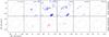 |
Fig. A.1 Channel maps of SiO(5–4) emission for the northern (top, color-coded blue) and southern (bottom, color-coded red) ALMA fields. Each map covers a 3.33 km s-1-wide velocity range indicated in the top row. First contour and interval are at 0.15 K km s-1. Compare to the equivalent maps for CO shown in Fig. 4. |
Appendix B: Comparison with a constant velocity model
To illustrate the need for a velocity gradient to fit the CO emission, we present here the results of a model that assumes constant velocity. This model uses the same parabolic shell geometry and gas parameters as the best-fit model presented in Sect. 4 with the only difference that its expansion velocity has a constant value of 11 km s-1. Figures B.1 and B.2 compare the predictions of this constant-velocity model with the ALMA observations, using the same maps used to compare the best-fit model with the data in Figs. 8 and 9.
As Fig. B.1 shows, the constant-velocity model predicts channel maps where the emission is distributed in a series of wedges that have their apex near the ellipse center and extend toward the ellipse boundary. At intermediate velocities, two symmetric wedges appear in each map, while only one wedge is present at extreme velocities.
The same wedge-like distribution of the velocity field can be seen in the first-moment map of Fig. B.2. This figure shows that the iso-velocity contours emerge radially from the ellipse center and have the ellipse minor axis as a plane of symmetry. This radial distribution of the contours is a direct consequence of the constant velocity field, which generates the different values of the radial velocity by simple projection. Since the ALMA data are inconsistent with this pattern, we can safely exclude a constant velocity of expansion.
In contrast with the channel and first moment maps, the integrated-intensity map shown in the left panels of Fig. B.2 presents a reasonable fit to the data. The map is in fact identical to that obtained with the best-fit model. This is expected because the emission is optically thin, so its integrated value depends only on the gas column density, which by construction is the same in the two models.
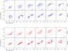 |
Fig. B.1 Comparison between observed velocity maps and results from a geometrical model that assumes constant velocity for both the northern (top and blue) and southern (bottom and red) ALMA fields. All labels and contours as in Fig. 8. |
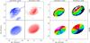 |
Fig. B.2 Comparison between maps of integrated intensity (left) and first momentum (right) from ALMA observations and a geometrical model that assumes constant velocity. All labels and contours as in Fig. 9. |
All Figures
|
Fig. 1 Large-scale image of the IRAS 04166 jet with circles representing the ALMA target positions. The color scale and contours represent the CO(2–1) EHV emission observed by SG09 with the IRAM PdBI, and the background grayscale is an archival Spitzer/IRAC1 image. The two 25′′ diameter circles represent the fields of view of the ALMA antennas. The B5, B6, and R6 labels indicate the emission peaks identified by SG09 and further studied in this paper. |
| In the text | |
|
Fig. 2 Comparison between the IRAM 30 m single dish spectra from T04 (blue and red histograms) and ALMA spectra synthesized for the same positions and angular resolution (11′′). The color vertical bands indicate the location of the blue and red EHV regimes. There is a good agreement between the 30 m and ALMA spectra inside the EHV ranges, which is indicative of only minor missing flux. IRAM 30 m data in Tmb scale and ALMA data in TB scale. |
| In the text | |
|
Fig. 3 Maps of the integrated EHV emission in the two ALMA target fields for the three main transitions in the setup: CO(2–1) (upper row of panels), SiO(5–4) (middle row), and SO(JN = 65–54) (bottom row). First contour and contour interval are 1.0 K km s-1 in the CO(2–1) maps and 0.5 K km s-1 in the SiO and SO maps. The dashed ellipses delineate the approximate boundaries of the CO emission. The small filled ellipses in the maps of the southern field indicate the synthesized beam for each transition. |
| In the text | |
|
Fig. 4 Channel maps of CO(2–1) emission for the northern (top, color-coded blue) and southern (bottom, color-coded red) ALMA fields. For each field, the maps cover the 20 km s-1-wide range shaded with color in Fig. 2. The velocity range of each map, after correction for a jet velocity of 37.5 km s-1, is indicated in the top row in units of km s-1. First contour and step are 20% of the map emission peak, which is indicated for each panel in the bottom left corner in units of K km s-1. The dashed ellipses delineate the approximate boundary of the emission. The emission from SW to NE is gradually displaced as the velocity increases. |
| In the text | |
|
Fig. 5 Schematic geometry of the emitting gas. The filled red circle indicates the position of IRAS 04166, and the green line is the direction of propagation of the jet. Each emitting region is represented by a tilted disk of gas that expands perpendicular to the jet axis, and whose velocity vectors have been color coded according to their Doppler shift. This schematic geometry simultaneously reproduces the elliptical shape of the emission and the systematic velocity pattern. (To improve visibility, the size of the disks has been exaggerated in proportion to their distance from the central source.) |
| In the text | |
|
Fig. 6 Evidence of curvature in the CO(2–1) emitting regions. Top panels: comparison between the CO emission in the reddest and bluest 5 km s-1 intervals of the EHV range for each ALMA field. First contour and contour interval are 0.5 K km s-1. Bottom panels: first moment maps of the CO(2–1) emission. As in Fig. 4, the velocity scale has been centered on zero by correcting for the source and jet velocities. Data outside the elliptical regions have been masked out as a result of their low signal-to-noise ratio. The wedge to the right shows the scale in km s-1. |
| In the text | |
|
Fig. 7 Schematic view of the shell used to model the emission in the southern ALMA field (the northern model is just the reflection image with respect to central source). As in Fig. 5, the green line represents the jet axis and the velocity vectors have been color coded according to their Doppler shift. |
| In the text | |
|
Fig. 8 Comparison between observed velocity maps and results from a geometrical model for both the northern (top and blue) and southern (bottom and red) ALMA fields. Both fields have been modeled assuming the same physical conditions but opposite orientation, as expected for two bow shocks moving away from the central IRAS source. Panel velocities, dashed ellipses, and contour levels as in Fig. 4. |
| In the text | |
|
Fig. 9 Comparison between maps of integrated intensity (left) and iso-velocity (right) from ALMA observations and the geometrical model presented in the text. For each comparison, the top panels represent the ALMA observations and the bottom panels represent the model. Each comparison uses the same velocity interval and contour levels as in Fig. 3 (integrated maps) and Fig. 8 (iso-velocity maps). |
| In the text | |
|
Fig. A.1 Channel maps of SiO(5–4) emission for the northern (top, color-coded blue) and southern (bottom, color-coded red) ALMA fields. Each map covers a 3.33 km s-1-wide velocity range indicated in the top row. First contour and interval are at 0.15 K km s-1. Compare to the equivalent maps for CO shown in Fig. 4. |
| In the text | |
|
Fig. B.1 Comparison between observed velocity maps and results from a geometrical model that assumes constant velocity for both the northern (top and blue) and southern (bottom and red) ALMA fields. All labels and contours as in Fig. 8. |
| In the text | |
|
Fig. B.2 Comparison between maps of integrated intensity (left) and first momentum (right) from ALMA observations and a geometrical model that assumes constant velocity. All labels and contours as in Fig. 9. |
| In the text | |
Current usage metrics show cumulative count of Article Views (full-text article views including HTML views, PDF and ePub downloads, according to the available data) and Abstracts Views on Vision4Press platform.
Data correspond to usage on the plateform after 2015. The current usage metrics is available 48-96 hours after online publication and is updated daily on week days.
Initial download of the metrics may take a while.