| Issue |
A&A
Volume 597, January 2017
|
|
|---|---|---|
| Article Number | A97 | |
| Number of page(s) | 14 | |
| Section | Extragalactic astronomy | |
| DOI | https://doi.org/10.1051/0004-6361/201629409 | |
| Published online | 10 January 2017 | |
Bulges and discs in the local Universe. Linking the galaxy structure to star formation activity
Excellence Cluster Universe, Boltzmannstr. 2, 85748 Garching bei München, Germany
e-mail: This email address is being protected from spambots. You need JavaScript enabled to view it.
Received: 27 July 2016
Accepted: 17 November 2016
Abstract
We use a sample built on the SDSS DR7 catalogue and the bulge-disc decomposition of Simard et al. (2011, ApJS, 196, 11) to study how the bulge and disc components contribute to the parent galaxy’s star formation activity, by determining its position in the star formation rate (SFR) – stellar mass (M⋆) plane at 0.02 < z < 0.1 and around the main sequence (MS) of star-forming galaxies. For this purpose, we use the bulge and disc colours as proxy for their SFRs, while the total galaxy SFR comes from Hα or D4000. We study the mean galaxy bulge-total mass ratio (B/T) as a function of the residual from the MS (ΔMS) and find that the B/T-ΔMS relation exhibits a parabola-like shape with the peak of the MS corresponding to the lowest B/Ts at any stellar mass. The lower and upper envelope of the MS are populated by galaxies with similar B/T, velocity dispersion and concentration (R90/R50) values. The mean values of such distributions indicate that the majority of the galaxies are characterised by classical bulges and not pseudo-bulges. Bulges above the MS are characterised by blue colours or, when red, by a high level of dust obscuration, thus indicating that in both cases they are actively star forming. When on the MS or below it, bulges are mostly red and dead. At stellar masses above 1010.5M⊙, bulges on the MS or in the green valley tend to be significantly redder than their counterparts in the quiescence region, despite similar levels of dust obscuration. This could be explained with different age or metallicity content, suggesting different evolutionary paths for bulges on the MS and green valley with respect to those in the quiescence region. The disc g−r colour anti-correlates at any mass with the distance from the MS, getting redder when approaching the MS lower envelope and the quiescence region. The anti-correlation flattens as a function of the stellar mass, likely due to a higher level of dust obscuration in massive SF galaxies. We conclude that the position of a galaxy in the Log SFR – Log M⋆ plane depends on the star formation activity of its components: above the MS both bulge and disc are actively star forming. The nuclear activity is the first to be suppressed, moving the galaxies on the MS. Once the disc stops forming stars as well, the galaxy moves below the MS and eventually to the quiescence region. This is confirmed by a significant percentage (~45%) of passive galaxies with a secure two component morphology, coexisting with a population of pure spheroidals. Our findings are qualitatively in agreement with the compaction-depletion scenario, in which subsequent phases of gas inflow in the centre of a galaxy and depletion due to high star formation activity move the galaxy across the MS before the final quenching episode takes place.
Key words: galaxies: evolution / galaxies: bulges / galaxies: star formation / galaxies: structure / galaxies: spiral
© ESO, 2017
1. Introduction
The main sequence (MS) of star-forming galaxies (SFGs) is a linear relation between the star formation rate (SFR) of a galaxy and its stellar mass (M⋆). This relation is close to linear, with a small scatter (0.2–0.3 dex) over a wide stellar mass range (e.g., Brinchmann et al. 2004; Noeske et al. 2007a,b; Daddi et al. 2007; Elbaz et al. 2007; Salim et al. 2007; Whitaker et al. 2012; Speagle et al. 2014; Pannella et al. 2015). It has also been shown that, while the slope of the relation remains ~1 up to z ~ 2, the normalisation changes drastically with redshift, where the SFR of galaxies at z ~ 2 is almost 20 times larger than that of galaxies at z ~ 0. (e.g., Schreiber et al. 2015). The physical processes that cause this decrease in SF activity are generally grouped under the term quenching, a topic at the core of galaxy evolution studies.
Quenching works by prohibiting SF in a galaxy and by acting on the cold gas reservoir. Processes that expel cold gas from galaxies, such as galactic winds driven by supernovae and massive stars are efficient in dark matter (DM) haloes with M< 1012M⊙ (e.g. Dekel & Silk 1986; Efstathiou 2000). Above this mass threshold, more powerful outflows are required to counter the deeper DM halo potential well. In such haloes, accreting central BHs can quench star formation by either heating the gas in the disc (quasar mode; Hopkins et al. 2006a,b; Dunn et al. 2010; Feruglio et al. 2010; Fabian 2012; Cicone et al. 2014), or mechanically removing the gas from the inner regions through powerful radio jets (radio mode; Croton et al. 2006; Bower et al. 2006, 2008; De Lucia et al. 2006; McNamara & Nulsen 2007; Vogelsberger et al. 2013; Di Matteo et al. 2005; Ciotti et al. 2007; Cattaneo et al. 2009). Besides ejecting the gas, the effects of quenching can also be caused by a lack of cold gas supply. In DM halos with M> 1012M⊙, the transition from cold to hot accretion (Dekel & Birnboim 2006) would prohibit further SF (Cen 2014). On the other hand, Martig et al. (2009) propose morphological quenching where the growth of central mass concentration, i.e. a massive bulge, could simply stabilise a gas disc against fragmentation, thus preventing SF without affecting the cold gas reservoir in the galaxy. It has also been proposed that quenching could be a combination of all these processes. For example, using their cosmological zoom-in simulations, Zolotov et al. (2015) show that quenching of high redshift SFGs is preceded by a compaction phase that creates the so-called blue nuggets: SFGs morphologically similar to quiescent ones. This compaction phase is caused by strong inflows to the centre due to minor mergers and/or counter-rotating gas and violent disc instabilities. The availability of dense cold gas in the centre results in a high SF and consequent stellar/supernova and/or AGN feedback causing quenching. Tacchella et al. (2015) propose that episodes of compaction, quenching and replenishment are responsible for the position of a galaxy in a ±0.3 dex region around the MS. The final quenching happens when the replenishment time is longer than the depletion time (i.e. in massive haloes, or at low redshifts) and results in a passive galaxy.
Observational evidence in favour of this scenario increased in the past years. The SFGs at z ≳ 2 characterised by the largest central gas densities seem to have spheroidal morphologies similar to the one of passive galaxies at the same redshift (Wuyts et al. 2011; Barro et al. 2014; Patel et al. 2013; Stefanon et al. 2013; Williams et al. 2013), but are significantly different from other SFGs (with lower central gas densities), which at z ≳ 2 are mostly irregular and clumpy (Elmegreen et al. 2004; Genzel et al. 2008; Guo et al. 2015b). At low redshift, less massive SFGs are mainly pure discs, while more massive SFGs are characterised by a bulge plus disc structure (Wuyts et al. 2012; Bruce et al. 2012, 2014; Lang et al. 2014). Wuyts et al. (2011) analyse the dependence of galaxy structure (size and Sérsic index) on the position of the galaxies with respect to the MS ridge at z = 0−2. They find that the Sérsic index tends to be roughly the same, n ~ 1, within 3σ from the MS, i.e., there is no significant gradient of n across the MS. They observe an increase of n only in the starburst region. While Cheung et al. (2012) confirm that the Sérsic index most sharply discriminates between the red sequence and the blue cloud, they also find a large number of blue outliers (≈40%) in their n > 2.3 galaxy sample at z ~ 0.65. Concurrently, using a sample of local galaxies Guo et al. (2015a) report that that bulges/bars are responsible for the large dispersion of the specific SFR (sSFR), but only for massive SFGs. These recent results imply that a significant percentage of SFGs must have a bulge plus disc morphology. Under the assumption that the star formation activity is confined in the disc, Abramson et al. (2014) show that defining the sSFR with respect to the disc mass rather than the total galaxy mass decreases (and sometimes erases) the dependence of sSFR on stellar mass. This suggests that the slope of the sSFR – M⋆ relation reflects the increase of the bulge prominence with stellar mass, and also points towards the importance of treating galaxies as multicomponent systems.
The aim of this paper is to study the relation between galaxies structural parameters and location with respect to the MS in the local Universe. The choice of performing this study on a local galaxy sample is dictated by the fact that the Sloan Digital Sky Survey (SDSS; Strauss et al. 2002) provides the required statistics to dissect the MS brick by brick to study the nature of its scatter as a function of the galaxy morphology with high accuracy. In addition, the availability of accurate morphological classification and bulge/disc decomposition (Simard et al. 2011) of the SDSS galaxies allows us to study the role and interconnection of the individual galaxy components. This is the first paper of a series, which follows the evolution of the relation of the galaxy structural parameter and scatter across the MS in the 0−2.0 redshift window.
The paper is organised as follows. In Sect. 1 we describe our dataset. In Sect. 2 we analyse the reliability of the morphological classification and colours of the bulge and disc in individual galaxies. In Sect. 3 we present our results and in Sect. 4 we present our discussion and conclusions. Throughout the study, the following cosmology is assumed: H0 = 70.0 km s-1 Mpc-1, Ωm = 0.3 and ΩΛ = 0.7.
2. Dataset
In this paper we make use of the catalogues derived from the SDSS-DR7 database (Abazajian et al. 2009) and in particular the following quantities: SFRs, stellar masses, stellar velocity dispersion, and properties derived from bulge/disc decomposition of galaxies. We now briefly summarise how these were derived and provide references to the original papers for details.
2.1. SFRs, stellar masses, and velocity dispersion
SFRs and M⋆ are taken from the MPA/JHU DR7 catalogues (Kauffmann et al. 2003; Brinchmann et al. 2004; Salim et al. 2007). In particular, we use the total, aperture corrected, stellar mass computed from the total ModelMag photometry that is less sensitive to emission line contamination. SFRs come from emission line modelling using the grid of ~2 × 10⁵ models of Charlot & Longhetti (2001), where dust corrections are mainly based on the Hα/Hβ ratio. The stellar aperture velocity dispersion σap (computed from stars) and mean signal-to-noise ratio (S/N) per pixel are taken from the MPA/JHU gal_info catalogue, while values of the Hα and Hβ fluxes and their S/Ns are from the MPA/JHU gal_line catalogue.
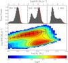 |
Fig. 1 Distribution of galaxies in SALL sample in the Log SFR – Log M⋆ plane. Top panels: SFR distribution of galaxies in three different stellar mass bins. The red solid line is the result of the gaussian fit to the right-side of the SF peak. Bottom panel: Log SFR – Log M⋆ plane colour-coded as a function of the number of galaxies in each bin. The contours encircle bins that host a number of galaxies from 50 to 1250, with step of 250. The MS of SFGs is indicated by the thick solid line, while the error bars mark the 1σ scatter. |
2.2. The bulge/disc decomposition catalogue
Galaxy structural parameters are taken from the bulge/disc decomposition of the Simard et al. (2011) catalogue (S11 hereafter). In S11, the GIM2D code (Simard et al. 2002) has been applied to the g and r filter images of 1 123 718 SDSS DR7 galaxies to obtain a two-dimensional bulge-disc decomposition convolved with the point-spread function. The simultaneous fit of the g and r images makes the decomposition robust against spurious effects. S11 provide structural parameters for three different fitting models: 1) a pure Sérsic; 2) an exponential disc plus De Vaucouleurs bulge; and 3) an exponential disc plus free Sérsic bulge model. In this work, we use the catalogue obtained from the exponential disc plus De Vaucouleurs bulge model as the F statistics reveal that SDSS images are not good enough to efficiently compute the Sérsic index of the bulge and its structural parameters (see S11 for details). We use the bulge-total ratio (B/T) computed from the r-band image and the magnitudes of the bulge and disc components, that are given as rest-frame, extinction, and K corrected. Extinction values are taken from the SDSS pipeline, while K correction was computed using version 4.2 of k-correct Blanton & Roweis (2007). We use the criterion PPS ≤ 0.32 (as suggested by S11) to select robust subsamples of genuine bulge plus disc systems, where PPS is the probability that a two-component model is not statistically needed to fit the galaxy image.
2.3. The galaxy sample
We construct the master catalogue from the MPA-JHU SFR and M⋆ catalogue, after removing duplicates and objects with no SFR or M⋆ estimates, and cross-correlate it with the S11 catalogue. Less than 2% of galaxies do not have a SFR or a stellar mass estimate because of low quality photometric or spectroscopic data. In the cross-correlation between the master and the S11 catalogues, only 8% of galaxies are lost owing to minor differences in the selection criteria applied in S11. To limit our analysis to a local volume galaxy sample with relatively high spectroscopic completeness, we select galaxies that satisfy the following criteria: 0.02 < z < 0.1, Log M⋆ ≥ 9.0M⊙, no AGN as identified in the MPA-JHU catalogue, and a good estimate of z and SFR.
Our selection criteria lead to a final galaxy sample of ~265 000 galaxies, SALL. In the bottom panel of Fig. 1 we show how galaxies in our SALL sample populate the Log SFR – Log M⋆ plane. In the upper panels we show the distribution of the SFR of galaxies in three bins of stellar mass to better visualise the typical bimodal distribution and its dependency on stellar mass. The thick solid line and error bars in the bottom panel of Fig. 1 indicate the position of the MS of SFGs and its 1σ scatter, respectively. Following the example of Renzini & Peng (2015), the MS and its scatter are computed as the mode and dispersion of the SFR distribution in several stellar mass bins. We divide the sample in stellar mass bins of 0.2 dex in the range 9.0 ≤ Log(M⋆/M⊙) ≤ 11.0. In each bin, we fit with a Gaussian to the right side of SFR distribution (see, as an example, the red fits in the upper panels of Fig. 1), to avoid shift in the peak value caused by the green valley population. We did not compute the MS values for masses M⋆ > 1011M⊙ since in this range the distribution is significantly non–Gaussian (Erfanianfar et al. 2016; Whitaker et al. 2012) and cannot be easily disentangled from the tail of the quiescent distribution. The mean (μ) and sigma (σ) values of the Gaussian fit are used as MS and scatter in the midpoint of each stellar mass bin and are summarised in Table 1.
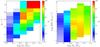 |
Fig. 2 Completeness in the (g−r) – Log M⋆ plane (left panel) and Log SFR – Log M⋆ plane (right panel) of the spectroscopic SALL sample with respect to the parent photometric Sphot sample. |
Main sequence SFRs (first column) and dispersion values (second column) in bins of stellar mass, in Log (M/M⊙) (third column).
To check for biases introduced by our selection criteria, we study the completeness of our spectroscopic SALL sample in the Log SFR – LogM⋆ plane, by comparing it with the parent photometric sample drawn from the SDSS DR7 in the same region, redshift, and stellar mass range (Sphot). The stellar masses for Sphot galaxies without spectroscopic data are derived from the z band absolute magnitude, Mz, using the best-fit Log M⋆−Mz relation obtained for SALL (Log(M⋆/M⊙) = (−0.42 ± 0.1)Mz + 1.3(±0.2)). On the other hand, obtaining a measure of the SFR without spectroscopic data is not trivial. We verified that the five SDSS broadbands are insufficient to retrieve a reliable measure of the SFR through the SED fitting technique. Also, the addition of the GALEX UV bands does not help in obtaining a reliable dust correction. Indeed, the scatter between the SFR derived in this manner and the SFR derived from the dust-corrected Hα emission of the MPA-JHU catalogue exceeds 0.5 dex. To overcome this issue we use the rest-frame (g−r) galaxy colour as a proxy for star formation activity.
The left panel of Fig. 2 shows the (g−r) – Log M⋆ plane colour-coded as a function of the completeness level of SALL with respect to Sphot. The completeness in each bin is estimated as the percentage of Sphot galaxies that are also in the SALL sample in the same bin. Completeness is below 50% for 109.0M⊙ < M⋆ < 1010.0M⊙. In this stellar mass range it is larger for blue, SFGs than for passive, redder galaxies because of the presence of strong emission lines. For M⋆ > 1010.0M⊙, the completeness is larger for redder galaxies, most likely owing to the strong stellar continuum. To obtain the completeness in the Log SFR – Log M⋆ plane we proceed as follows. For every galaxy we get the completeness value by its (g−r) colour and stellar mass (left panel). We then compute the completeness in a given bin of the Log SFR – Log M⋆ as the average completeness over all galaxies in that bin. The result is shown in the right panel of Fig. 2. Completeness varies between 5% and ~20% for galaxies with M⋆ < 109.5M⊙, where it is larger for blue, SFGs owing to the presence of strong emission lines. For stellar masses in 109.5−10.0M⊙, the completeness of the spectroscopic catalogue reaches 40% on the MS and in its upper envelope, while it decreases to 20% for passive galaxies. For galaxies with M⋆ > 1010M⊙, completeness is always higher than 60%, reaches values of ~80% on the MS, and is even larger in the passive region with M⋆ ~ 1010.5−11.0M⊙, where galaxies are characterised by a strong continuum.
2.4. Bulge/disc decomposition reliability: comparison with BUDDA and Galaxy Zoo
To check the reliability of the S11 B/T classification, we compare it with different morphological classifications, in particular, BUDDA (de Souza et al. 2004, Bulge/disc Decomposition Analysis) and Galaxy Zoo (Lintott et al. 2008). Both classifications take the presence of bars into account. Thus, this comparison is particularly interesting to understand how the presence of a bar can bias the S11 B/T estimate.
BUDDA is a fortran code that performs multicomponent decomposition of galaxies. Bulges are fitted with Sérsic profiles and discs are fitted with exponentials. Unlike in GIM2D, in addition to bulge and disc, bars are also modelled with a Sérsic profile. We make use of the public catalogue of structural parameters presented in Gadotti (2009, G09 hereafter), where the BUDDA code has been applied to a sample of 946 spectroscopically confirmed, nearly face-on galaxies, in the range 0.02 ≤ z ≤ 0.07 and M⋆ > 1010M⊙. The final sample of G09 is clean and optimal for bulge/disc decomposition as the quality of each image has been inspected by eye and the redshift range is low. The S11 and G09 catalogues have 910 galaxies in common (correlation radius r = 3″). We compare the B/T ratios of S11 (B/TGIM2D) with the G09 values (B/TBUDDA). Both B/T values have been computed from the r-band images. Results are shown in Fig. 3. The red stars are the median values of the whole sample in bins of 0.1 in B/T and the errors are computed as the standard deviation in each bin. We find an overall agreement between the two methods at least below B/T ~ 0.6. GIM2D tends to find slightly higher B/Ts with respect to BUDDA. The blue triangles indicate the subsample of galaxies that are classified as “barred” in BUDDA, while the black circles indicate the “unbarred” subsample. A very good agreement in B/TBUDDA and B/TGIM2D is found for unbarred galaxies, while for barred galaxies, GIM2D tends to estimate higher values of the B/T of almost double at B/T < 0.1 and 20−30% higher at larger B/Ts. Despite this, the overall effect is not dramatic as B/TGIM2D for the whole sample (red stars) does not increase more than 25% because of the inclusion of barred galaxies. This is because of their relatively low percentage, ~30%. Above the B/T ~ 0.6 threshold, B/TGIM2D tends to flatten to an average value of ~0.7. This is consistent with the tendency of GIM2D to find an overabundance of small discs in spheroidal galaxies, as pointed out in S11.
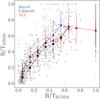 |
Fig. 3 Comparison between B/TBUDDA and B/TGIM2D. The red stars are the median value of the B/TGIM2D in bins of 0.1 B/TBUDDA for all galaxies that the two catalogues have in common, while the blue triangles and black circles are used for the subsamples of barred and unbarred galaxies, respectively. The error bars are given by the standard deviation in each bin. |
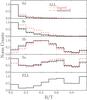 |
Fig. 4 Distribution of the S11 B/T in the different morphological classes defined by Galaxy Zoo 2 (from top to bottom: Sd, Sc, Sb, Sa, and ellipticals). The histograms have been normalised to the peak. The red dashed histograms describe barred spirals, while the black dashed histograms indicate unbarred spirals. The whole population of barred and unbarred galaxies is described by the black solid histograms. |
We compare GIM2D with the second release of Galaxy Zoo (Lintott et al. 2008), which is a project aimed at classifying “bye-eye” the morphology of galaxies in the SDSS Main Galaxy Sample (Strauss et al. 2002). The catalogue provides morphological classification only for ~50% of the parent photometric sample drawn from the SDSS. The remaining half of the galaxy sample is classified with uncertain morphology. In the second release (GZ2; Willett et al. 2013) ellipticals are classified as round, cigar-like, or in-between. Spirals are classified in four classes as a function of the bulge prominency: Sa if they have dominant bulge, Sb for obvious bulges, Sc if the bulge is just noticeable, and Sd if there is no bulge. In addition, spirals are also divided into barred and not-barred categories. Since edge-on spirals have separate morphological classes in GZ2, we restrict this analysis to galaxies that, in S11, have a disc inclination angle that is smaller than 70° (where i = 90° for an edge-on disc). In Fig. 4, we show the B/T distribution of each subcategory, which are identified using the gz2class final classification in GZ21. The GZ2 ellipticals, which are considered as a whole regardless of the shape, are characterised by a B/T distribution peaking at B/T ~ 1 and with a second peak at B/T ~ 0.6. We also observe a third, much less significant peak at B/T of 0. Approximately 60% of GZ2 ellipticals with B/T < 0.8 have PPS ≤ 0.32, thus making the disc component statically significant. These galaxies could be S0 galaxies that are visually misclassified as ellipticals (Willett et al. 2013; Huertas-Company et al. 2011). Not surprisingly, for GZ2 Sa galaxies, i.e. consistent with an intermediate morphology template (bulge-dominated spiral), the B/T distribution is wide with three peaks, at B/T of 0, ~0.5, and 1, respectively. However, we point out that Sa galaxies account only for less than ~1% of the GZ2 sample. For Sb, Sc, and Sd the B/T distributions reveal a very good agreement between GZ2 and GIM2D classification. Also, it is clear from Fig. 4 that the presence of a bar (red dashed line histograms) results in an overestimate of the GIM2D B/T, in particular for Sc and Sd galaxies.
We point out that neither G09 or GZ2 catalogues are suitable for our analysis. While BUDDA does not provide the required statistics, in GZ2, the visual classification is available only for half of the parent galaxy subsample drawn from the SDSS, leading to a high level of incompleteness. Only S11simultaneously provides the required statistics and completeness.
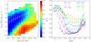 |
Fig. 5 Left panel: Log SFR – Log M⋆ plane colour-coded according to the weighted average B/T in the bin. The white line represents the location of the MS of SFGs, and the error bars indicate its dispersion. Right panel: B/T ratio as a function of ΔMS (distance from the MS) in different stellar mass bins. The dotted vertical line indicate the position of the MS. Error bars are obtained via bootstrapping. |
The drawback of using S11 is the uncertainty of bulge/disc decomposition at relatively high values of B/T. Indeed, the comparison with BUDDA and GZ2 shows that S11 find an overabundance of double component systems among galaxies that are classified as pure spheroidal by BUDDA and by the visual classification. Cheung et al. (2013) suggest that among galaxies with B/T > 0.5 only those with PPS < 0.32 have a reliable the bulge/disc decomposition. However, such a drastic cut would imply selecting only half of the S11 sample at B/T > 0.5, leading to significant selection effects in our analysis. To overcome this problem, we adopt the following approach. When measuring the mean B/T in the Log SFR – Log M⋆ plane, we use a weighted mean, where the weights are based on the errors provided by the S11 catalogue for B/T. Including this error in the weighted mean allows us to take into account the uncertainty due to low S/N and resolution issues. This approach also allows us to propagate the uncertainty of the morphological classification throughout our analysis. As an alternative approach, and to verify the robustness of our results, we create a reference sample (Sref) in which we keep the B/T as given by S11 for all galaxies with PPS ≤ 0.32. Instead, galaxies that have PPS > 0.32 are consider as pure disks (B/T = 0) when B/T ≤ 0.5 or as pure spheroidals (B/T = 1) when B/T > 0.5. The results based on Sref are shown for comparison in Appendix A. When analysing the colours of the individual components in the Log SFR – Log M⋆ plane, we use a sample with robust double component classification by imposing the cut at PPS < 0.32.
3. Results
In the following sections, we study the galaxy B/T and bulge/disc colours in the Log SFR – Log M⋆ plane. The purpose of this analysis is to better understand the drivers of the MS scatter, and the main differences in galaxy properties between SF and passive galaxies.
3.1. The B/T across the Log SFR – Log M⋆ plane
In Fig. 5 we show the distribution of the B/T values of SALL in the Log SFR – Log M⋆ plane (left panel). Each bin is colour-coded according to the weighted average of the B/Ts in that bin. The width of each bin is 0.2 in both Log M⋆ and Log SFR to account for the average errors with a minimum of 20 galaxies per bin. The white solid line is the MS and the error bars show the dispersion around it (Table 1).
Figure 5 confirms the result already obtained by Wuyts et al. (2011): the MS is populated mainly by disc-dominated galaxies and the quiescent region by bulge-dominated systems. Intermediate B/T values are found in the green valley and the upper envelope of the MS. We also confirm previous results that the mean B/T on the MS increases as a function of the stellar mass, going from 0.16 at 10.2 < Log M⋆ < 10.4, to 0.21 at 10.4 < Log M⋆ < 10.6, 0.26 at 10.6 < Log M⋆ < 10.8, and 0.32 at 10.8 < Log M⋆ < 11.0. This implies that the MS above Log M⋆ = 10.2 begins to be populated by double component galaxies, which is consistent with previous findings (Lang et al. 2014; Bluck et al. 2014; Erfanianfar et al. 2016). When approaching the quiescence region at ≳1 dex below the MS, the B/T further increases to reach an average value between 0.6−0.7 for galaxies with Log M⋆ > 9.6. For less massive galaxies, the average B/T in the passive region is in the range 0.3–0.5. However, this is the region most affected by completeness issues as shown in Fig. 2. Thus, it is very likely that a strong selection effect in favour of emission line galaxies is biasing the mean value of the B/T in the weighted mean.
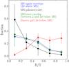 |
Fig. 6 Fraction of galaxies as a function of the B/T within the MS (black circles), in the upper envelope of the MS (blue stars), in the green valley, and in the passive region (red triangles). The fraction is estimated as the mean in several bin of stellar mass from 1010 to 1011M⊙. The error bars show the dispersion around the mean. The MS upper envelope and the lower envelope (green valley) share the same distribution of galaxies as a function of the B/T: ~40% of the population has B/T > 0.4 vs. 15% of the galaxies in the MS. |
A deeper insight is obtained from a careful analysis of the relation between the residuals around the MS, ΔMS = Log SFRMS – Log SFRgal (where SFRMS is the SFR on the MS and SFRgal is the galaxy SFR), and the mean B/T in different stellar mass bins as shown in the right panel of Fig. 5. Contrary to Wuyts et al. (2011), who find a roughly constant value of the Sérsic index n ~ 1 around the MS, we observe that the B/T-ΔMS relation exhibits a parabola-like shape within 3σ from the MS with the MS coinciding with the lowest B/Ts at any stellar mass. In contrast to previous results (Wuyts et al. 2011; Cheung et al. 2012), we find that star-forming blue galaxies with a bulge-dominated morphology are not outliers in the diagram but are just populating the upper envelope tail of the MS. To further investigate how galaxies with different morphologies populate the plane, we study the distribution in the entire stellar mass range of the B/T for galaxies above the MS (>2σ), within the MS (±2σ), in the lower envelope of the MS (2−3σ below) and in the passive region (3σ below). As shown in Fig. 6, the MS (black line) is dominated by pure disc galaxies, in which ~60% of the population have B/T < 0.2. The large error associated with MS galaxies with B/T ≤ 0.2 reflects the increase of the B/T along the MS. In the upper envelope of the MS (blue stars), disc galaxies make up only ~30% of the entire galaxy sample, favouring a population of intermediate B/Ts. Similarly, ~35% of galaxies are pure discs in the lower envelope of the MS. Galaxies in the lower and upper envelopes of the MS share the same distribution of galaxy B/T. Among passive galaxies (red triangles), ≈70% have B/T ≤ 0.8. As discussed earlier, this fraction is contaminated by true spheroidal galaxies for which GIM2D finds a spurious disc. Nevertheless, there is a significant population of passive galaxies with a secure bulge plus disc morphology, as ≈45% of all passive galaxies have B/T ≤ 0.8 and PPS < 0.32. Also, the fraction of passive galaxies with B/T < 0.2 is negligible, indicating that passive pure discs, if at all present, are outliers of the galaxy population.
These trends of B/T in the Log SFR – Log M⋆ are also confirmed using the Sref sample (see Appendix A). As an additional test, we repeat the analysis by limiting the sample to galaxies with high S/N photometric data and secure S11 classification, by selecting galaxies with a disc scale length larger than 2 arcsec to avoid resolution issues (as in Cheung et al. 2013). All the tests confirm the results presented in Fig. 5.
3.2. The effect of bars
In Sect. 2.4 we conclude that S11 and G09 show good agreement for B/T < 0.6 and that the presence of a bar leads to an overestimation of the S11 B/T of 10−25%. However, the gradient observed from the peak of the MS towards the upper and lower envelopes of the relation leads to an increase of the mean B/T by a factor ~3−5, depending on the stellar mass bin. Thus, the increase of the mean B/T across the MS is much larger than the overestimation of the B/T due to the bars. Nevertheless, the bars could be preferentially located in certain regions of the Log SFR – Log M⋆ plane, thus affecting the average B/T value of that region.
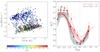 |
Fig. 7 Left panel: Log SFR – Log M⋆ plane for galaxies in the bulge-disc decomposition catalogue of G09. Each marker is colour-coded accordingly to the B/T value of the galaxy. Right panel: B/T as a function of the distance from the MS, ΔMS, for the G09 whole sample (shaded region), and for the G09 subsample of unbarred galaxies (solid lines). The sample was divided into two bins of stellar mass, 10.0 ≤ Log(M⋆/M⊙) < 10.5 (in black) and 10.5 ≤ Log(M⋆/M⊙) < 11.0 (in red). The B/T distributions computed for the SALL sample are also shown for comparison in dashed lines. The solid vertical lines indicates the location of the MS. error bars are obtained via bootstrapping. |
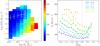 |
Fig. 8 Left panel: distribution of galaxies in the Log SFR – Log M⋆ plane, in which each bin (0.2 M⊙ in M⋆ and 0.2 M⊙ yr-1 in SFR) is colour-coded according to the weighted average value of the velocity dispersion σe in the bin. The white line represents the location of the MS of SFGs. Right panel: σe as a function of the distance from the MS, ΔMS, in six different bins of stellar mass, each 0.2 M⊙ wide. The different bins of stellar mass are indicated with different colours, as defined in the legend of the image, while the grey dotted vertical line represents the location of the MS. The error bars are obtained via bootstrapping. |
To check this, we perform the same analysis as in Fig. 5 on the G09 sample (see left panel of Fig. 7). We observe a ~25% milder increase of the mean B/T along the MS with respect to the result of Fig. 5 (mean B/T value of 0.13, 0.19, and 0.23 at stellar masses of 1010−10.4, 1010.4−10.8, and 1010.8−11.2M⊙, respectively), which is consistent with the overall effect of overestimation of the S11 B/T from the inclusion of barred galaxies. Because of the relatively small size of the G09 sample, the upper and lower envelopes of the MS are poorly populated. Thus, we limit the analysis of the mean B/T as a function of the distance from the MS to two stellar mass bins, above and below the median mass of the sample (1010.25M⊙). We perform the analysis for the whole G09 sample and for the “unbarred” G09 sample (deprived of barred galaxies). The right panel of Fig. 7 shows the mean B/T as a function of ΔMS for the two G09 samples in comparison with the mean relation obtained in the same stellar mass bins in S11. The error bars are estimated via bootstrapping technique. We find a perfect match of all relations in the MS region. This indicates that bars do not play a crucial role in the gradient of B/T across the MS. Only in the quiescence region, as expected, the S11 relation shows lower mean B/T with respect to G09 because of the underestimation of S11 B/T for spheroidal galaxies (Fig. 3). In addition the barred galaxy sample of G09 shows that the B/T-ΔMS for barred galaxies exhibits the same parabola-like shape. Thus, barred galaxies follow the same trend. This suggests that the presence of a bar on average plays a second order effect with respect to the galaxy morphology.
3.3. Velocity dispersion in the Log SFR – Log M⋆ plane
To investigate the similarities and differences of the bulgy galaxy population in the upper and lower limit of the MS, we use the bulge velocity dispersion, σ, and the SDSS concentration parameter, R90/R50. The parameters σ and R90/R50 are often used to discriminate between classical and pseudo-bulges (see e.g. G09). Classical bulges resemble spheroidal galaxies for their colours and scaling relations. Pseudo-bulges are, instead, outliers in the Kormendy relation (Kormendy 1977,G09). They tend to be blue and with low velocity dispersion with a Sérsic index close to ~2.
To retrieve the bulge velocity dispersion, we use the estimate of the stellar velocity dispersion provided by the MPA-MJU catalogue, which is measured by fitting the stellar absorption features of the SDSS galaxy spectra. The aperture velocity dispersion, σap, is computed inside the SDSS fibre, characterised by a 3 arcsec diameter. Such an aperture samples different galaxy parts as a function of redshift, galaxy size, and morphology. In order to sample the bulge alone, we select galaxies with B/T ≥ 0.5 and galaxies with PPS ≤ 0.32 if B/T< 0.5. In order to exclude contamination by disc rotation, we limit our analysis to nearly face-on galaxies, with disc inclination i< 30°2.
Given the spectral resolution of the SDSS spectrograph and typical S/N values, velocity dispersion estimates smaller than ~70 km s-1 are not reliable. Thus, to all galaxies with σap< 70 km s-1, we assign a fixed upper limit of σap = 70 km s-1 with an error of ±70 km s-1 to be used for the weight calculation in the weighted mean. We also exclude galaxies with σap> 420 km s-1 (as the SDSS template spectra are convolved to a maximum sigma of 420 km s-1) and with low S/N continuum (<3). We apply the aperture correction of Jorgensen et al. (1995) to σap to compute σe: the velocity dispersion within the effective radii of the galaxy, re (that we take from SDSS database). In the redshift range considered here, the average aperture correction is ~14%.
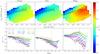 |
Fig. 9 Galaxy (left panels), disc (central panels), and bulge (right panels) colours in the Log SFR – Log M⋆ plane. In the upper panels, the distribution of galaxies in the Log SFR – Log M⋆ plane is colour-coded according to the weighted average (g−r) colour in each bin. The bins are 0.2 M⊙ in Log M⋆ and 0.2 M⊙ yr-1 in Log SFR. In the bottom panels, the (g−r) colour is shown as a function of the distance from the MS, ΔMS, in different bins of stellar mass, represented by different colours (same as Fig. 5). The error bars in the lower panels are obtained via a bootstrapping. |
Figure 8 shows the distribution of galaxies in the Log SFR – Log M⋆ plane colour-coded as a function of the average σe in each bin. The error bars in Fig. 8 are estimated via a bootstrapping analysis. The behaviour of σe across and along the MS is qualitatively similar to the B/T ratio. At a fixed stellar mass, σe has its minimum on the MS, increases towards the upper and lower envelopes of the MS, and reaches its maximum in the quiescence region. Also, the velocity dispersion of MS galaxies increases for increasing stellar mass along the MS, resembling the B/T behaviour. We point out that the exclusion of pure-disc galaxies, which populate the core of the MS, naturally leads to a flatter parabola-like shape for the σe−ΔMS distribution as a function of the mass.
The same trend in Fig. 8 is also observed for the concentration parameter, which is one of the most reliable discriminant (G09) between bulges and pseudo-bulges at given B/T (see Appendix B). In the lower and upper envelopes of the MS the mean value of R90/R50 ≈ 2.5 is consistent with the mean for classical bulges with low values of D4000, as estimated in the same mass range by G09 (see Fig. 20 of G09). Low values of the D4000 index would indicate a relatively young age of the stellar population. Values of R90/R50 ≈ 2, which are consistent with pseudo-bulges, are found only in the core of the MS. In the quiescence region, the mean R90/R50 ≈ 3 is consistent with classical bulges with high values of D4000, i.e. older stellar populations. Thus, we conclude that lower and upper envelopes of the MS share the same B/T, bulge velocity dispersion, and concentration parameter distributions. Both are populated by intermediate morphology galaxies with classical bulges. The similarity of these distributions could suggest that the scatter around the MS is characterised by different evolutionary stages of the same galaxy population, while the MS itself is mainly populated by pure disc galaxies.
3.4. Bulge and disc colours in the Log SFR – Log M⋆ plane
The SDSS spectroscopic dataset does not provide any spatial information. Thus to understand whether there is a connection between the SF activity of the individual galaxy components (bulge and disc) and the star formation of the galaxy as a whole, we use the colour of bulges and discs as a proxy of their SFR, while the total SFR of the galaxy is taken from Brinchmann et al. (2004). For this purpose we limit this analysis to the SALL sample with secure double morphological component, applying the cut at PPS ≤ 0.32.
In Fig. 9 we show the (g−r) colour of the galaxy (upper left panels), disc (upper central panels), and bulge (upper right panels) in the Log SFR – Log M⋆ plane. The upper panels are colour–coded as a function of the galaxy or galaxy component colour. The colour in each bin is obtained with a weighted mean. The bottom panels show the dependence of the mean colour of the whole galaxy (left panel), disc (central panel) and bulge (right panel) on the distance from the MS.
The galaxy and disc colours follow similar trends where at any stellar mass bin, they anti-correlate with the distance from the MS, getting progressively bluer from the quiescence region to the upper envelope of the MS. The anti-correlation is steeper for the whole galaxy colour than for the disc component. In both cases, the relation flattens progressively towards highest stellar mass bin. The bulge colour shows a different behaviour instead. Up to ~1010M⊙, the bulge colour also anti-correlates with the distance from the MS, getting bluer from the passive region to the upper envelope of the MS. In this stellar mass range bulges above the MS are as blue as their discs. However, above ~1010M⊙, the relation reverses with the bulge colour getting redder from the passive region up to the MS. After reaching its reddest value, the bulge turns slightly bluer towards the upper envelope of the MS. However, the bulge colour is always redder than the disc even in the upper envelope of the MS. For M > 1011M⊙, bulges are always characterised by red colours independent of their position on the Log SFR – Log M⋆ plane.
In order to check the bias from dust obscuration, we analyse the average Balmer decrement computed for galaxies with S/N > 8 in both Hα and Hβ (Fig. 10). Dust obscuration is not significant for galaxies with stellar masses below 1010M⊙. Hence the trends in colours reflect a trend in SF activity. Very massive (≳1010.5M⊙) SFGs in the upper MS envelope exhibit the highest values of Balmer decrement, pointing to a very high level of dust obscuration. This, in turn, would suggest that the flattening of the colour gradients across the MS at increasing stellar mass in all panels of Fig. 9 could be due to an increasing level of dust obscuration towards the upper envelope of the MS.
We also point out that above 1010.5M⊙, the very red colour of bulges in the green valley and on the MS cannot be explained by a large level of dust obscuration due to the low average Balmer decrement. We conclude that the bulges in massive MS and green valley galaxies are intrinsically redder than their counterparts in the passive region. This implies that such bulges might be older or more metal rich with respect to bulges in the passive region. In any case, this suggests different evolutionary paths for bulges on the MS, and in the passive region.
The observed trends of the bulge and disc colours at fixed stellar mass with the distance from the MS are also preserved when considering all galaxies in SALL with 0.2 ≤ B/T ≤ 0.8.
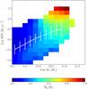 |
Fig. 10 Balmer decrement in the Log SFR – Log M⋆ plane for galaxies in our sample that have a median S/N per pixel >8. The white solid line and error bars represent the MS of SFGs and its dispersion. |
4. Discussion and conclusions
We used the bulge-disc decomposition of Simard et al. (2011) to study the link between the structural parameters of galaxies and their location in the Log SFR – Log M⋆ plane. We use the colour of bulges and discs to understand how these individual components influence the evolution of the galaxy as a whole. Our sample is drawn from the spectroscopic sample of SDSS DR7, in the redshift range 0.02 < z < 0.1 and M⋆ > 109M⊙, and the main findings are as follows:
-
The MS of SFGs is populated by galaxies that, at every stellarmass, have the lowest B/Ts. At low stellar masses, M⋆ < 1010.2M⊙, MS galaxies are pure discs, while the prominence of the bulge component increases with increasing stellar mass for more massive galaxies.
-
The upper and lower envelopes of the MS are populated by galaxies characterised by intermediate B/Ts. This is robust against different decompositions and independent of the modelling of the bar component.
-
Bulges in the upper envelope of the MS are characterised by blue colours at low stellar masses, or red colours and large dust obscuration at high stellar masses. This is consistent with high SF activity in the central region of the galaxy.
-
The study of the mean bulge velocity dispersion and galaxy concentration parameter indicates that galaxies populating the upper and lower envelopes of the MS are structurally similar. The values of the concentration parameter, in particular, suggest that these galaxies are characterised by classical bulges rather than pseudo-bulges.
-
In the low mass regime, M⋆ < 1010M⊙, disc and bulge colours show a similar behaviour at fixed stellar mass, becoming progressively redder from the upper envelope of the MS to the passive region. Nevertheless, the reddening of the bulge component is steeper than for discs. Discs and bulges become bluer for M⋆ > 1010M⊙ when going form the MS towards its upper envelope, despite a less pronounced total variation of colours. The trend of the bulge colour reverses in the lower envelope of the MS, where bulges are redder than in the passive region.
-
The population of passive galaxies is largely made of genuine bulge plus disc systems (at least 45%).
Our results point to a tight link between the distribution of galaxies around the MS and their structural parameters. Contrary to Wuyts et al. (2011) and Cheung et al. (2012), we find that blue bulgy SFGs are not outliers in the distribution of galaxies on the MS. They occupy the upper tail of the MS distribution, leading to a progressive increase in B/T above the MS. In particular, Wuyts et al. (2011) find that the galaxy Sérsic index remains ~1 in the region of the MS. We find, instead, that the MS location corresponds to the lowest value of the B/T at any mass. This could be due to the inability of a single Sérsic model (used in Wuyts et al. 2011) to capture small bulges in disc-dominated galaxies. In agreement with previous results, we find a large percentage of bulge-dominated systems in the high-mass SF region, where the MS scatter tends to increase (i.e. Lang et al. 2014; Whitaker et al. 2014; Erfanianfar et al. 2016). However, the B/T-ΔMS relation at fixed stellar mass holds in the stellar mass range 109−11M⊙, and seems to flatten where the MS itself tends to disappear. We also investigate how the presence of a bar influences the scatter around the MS. Overall we conclude that bars do not affect the scatter of the MS or the B/T−ΔMS relation. In fact, this relation holds for both the unbarred and barred G09 subsamples. This suggests, partly in disagreement with the findings of Guo et al. (2015a), that the predominance of the bulge in a galaxy is intrinsically related to the location of a galaxy around the MS, and this is true at any stellar mass independent of the presence of a bar. Nevertheless, we do not exclude the possibility that a large percentage of bars among very massive SFGs can contribute to an increase in the scatter of the MS, as suggested by Guo et al. (2015a).
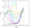 |
Fig. 11 B/T ratio, as a function of the distance from the MS, represented by the vertical dotted line. Here ΔMS was computed from the sSFR normalised to Mdisc. Different bins of stellar mass are indicated with different colours. |
Our study shows that the location of galaxies in the Log SFR – Log M⋆ plane and, in particular, with respect to the MS of SFGs, is determined by the combined activity (or inactivity) of the individual galaxy components. This was previously suggested by Abramson et al. (2014), who have pointed out that the MS becomes roughly linear if one assumes that the SF activity takes place only in the disc rather than in the entire galaxy. However, our results suggest otherwise. The effect of normalising the SF activity to the disc mass leads to a completely flat and tight relation only for pure disc galaxies, which, as shown here, dominate the core of the MS distribution. Extending this normalisation to galaxies of intermediate morphology has the additional effect of increasing the scatter by ~0.1 dex in any mass bin. We suggest the following explanation:  (1)thus,
 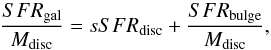 (2)
(2)
where Mdisc is the disc mass and sSFRdisc is the specific SFR of the disc. The last equation leads to the following effects:
-
For pure disc galaxies, which dominate the core of theMS, the mass of the disc equals the mass of the galaxy andSFRbulge ~ 0, hence SFRgal/Mdisc = sSFRdisc. Since the MS is nearly linear, sSFRdisc−M⋆ relation is flat with a very small scatter.
-
For intermediate B/T galaxies in the upper envelope of the MS, thus with a blue star-forming bulge, SFRbulge> 0 and Mdisc<Mstar. This implies that SFRgal/Mdisc = sSFRdisc + SFRbulge/Mdisc. Therefore such galaxies are displaced well above the sSFRdisc−M⋆ relation by the contribution of SFRbulge/Mdisc. The larger the SFR of the bulge, the larger the displacement.
-
For intermediate B/T galaxies in the lower envelope of the MS, thus with a red quiescent bulge, SFRbulge ~ 0, hence SFRgal/Mdisc = sSFRdisc. They scatter around the sSFRdisc −M⋆ relation in the same way as around the MS.
In Fig. 11, we show the relation between B/T and distance from the MS computed as the difference between the sSFRdisc of galaxies and sSFRdisc of galaxies in the MS. This is carried out for galaxies that are pure discs or have a secure bulge plus disc structure. The B/T trends in Fig. 11 are similar to those in Fig. 5; there is a steep increase of the mean B/T in the upper envelope of the MS due to the displacement of bulgy SFGs above the sSFRdisc −M⋆ relation. We underline that the B/T in the passive region is lower than that observed in Fig. 5, as here pure spheroidal galaxies are excluded from the sample. We find that the overall effect of neglecting the SF activity of the bulge component is to increase the scatter of the sSFR – M⋆ relation.
It has been proposed that minor mergers or violent disc instabilities could favour the flow of cold gas from the disc towards the galaxy centre and, thus, cause an overall compaction of the system. The high SF activity in the centre would lead to a compact, bulgy, star-forming object (Dekel & Burkert 2013; Zolotov et al. 2015). Tacchella et al. (2015) study the evolution of galaxies in this scenario using zoom-in simulations and they find that galaxies at high redshift undergo subsequent phases of compaction and depletion of the gas reservoir, which ultimately leads to quenching. The compaction phase causes high SF in the central region of galaxies, and hence could favour bulge growth. This phase is then followed by depletion from gas exhaustion. Such subsequent phases can move a galaxy across the MS: towards the upper envelope during compaction and towards the lower envelope during depletion. Complete quiescence can be reached once the bulge reaches a given mass threshold corresponding to no more inflows in massive halos or AGN feedback. Our findings on the B/T in the Log SFR – Log M⋆ plane and bulge/disc colours can be related to such a scenario and are also consistent with the observed gradient of molecular and atomic gas fraction across the MS, as seen by Saintonge et al. (2016).
Integral field spectroscopy surveys, such as MaNGA (Bundy et al. 2015) and CALIFA (Sánchez et al. 2012), will greatly advance our understanding of the evolution of individual galaxy components, and how they impact the galaxy as a whole. This will help us draw a better picture of the quenching mechanism, and understand the CSFH at any epoch.
Alternatively, a similar comparison can be carried out using the vote fractions instead of the gz2class parameter, but this leads to a decrease in the number of sources for the comparison, especially in the case of intermediate-morphology galaxies.
The disc inclination angle is 0° for face-on galaxies and 90° for edge-on galaxies.
Acknowledgments
We thank the anonymous referee for useful comments that improved the manuscript. This research was supported by the DFG cluster of excellence “Origin and Structure of the Universe”. L.M. thanks Alvio Renzini and Pieter van Dokkum for their useful comments on the project. L.M. would also like to thank Bhaskar Agarwal for his inputs on the manuscript.
References
- Abazajian, K. N., Adelman-McCarthy, J. K., Agüeros, M. A., et al. 2009, ApJS, 182, 543 [NASA ADS] [CrossRef] [Google Scholar]
- Abramson, L. E., Kelson, D. D., Dressler, A., et al. 2014, ApJ, 785, L36 [NASA ADS] [CrossRef] [Google Scholar]
- Barro, G., Faber, S. M., Pérez-González, P. G., et al. 2014, ApJ, 791, 52 [NASA ADS] [CrossRef] [Google Scholar]
- Blanton, M. R., & Roweis, S. 2007, AJ, 133, 734 [NASA ADS] [CrossRef] [Google Scholar]
- Bower, R. G., Benson, A. J., Malbon, R., et al. 2006, MNRAS, 370, 645 [NASA ADS] [CrossRef] [Google Scholar]
- Bower, R. G., McCarthy, I. G., & Benson, A. J. 2008, MNRAS, 390, 1399 [NASA ADS] [Google Scholar]
- Brinchmann, J., Charlot, S., White, S. D. M., et al. 2004, MNRAS, 351, 1151 [NASA ADS] [CrossRef] [Google Scholar]
- Bruce, V. A., Dunlop, J. S., Cirasuolo, M., et al. 2012, MNRAS, 427, 1666 [NASA ADS] [CrossRef] [Google Scholar]
- Bruce, V. A., Dunlop, J. S., McLure, R. J., et al. 2014, MNRAS, 444, 1660 [NASA ADS] [CrossRef] [Google Scholar]
- Bundy, K., Bershady, M. A., Law, D. R., et al. 2015, ApJ, 798, 7 [NASA ADS] [CrossRef] [Google Scholar]
- Cattaneo, A., Faber, S. M., Binney, J., et al. 2009, Nature, 460, 213 [NASA ADS] [CrossRef] [PubMed] [Google Scholar]
- Cen, R. 2014, ApJ, 789, L21 [NASA ADS] [CrossRef] [Google Scholar]
- Charlot, S., & Longhetti, M. 2001, MNRAS, 323, 887 [NASA ADS] [CrossRef] [Google Scholar]
- Cheung, E., Athanassoula, E., Masters, K. L., et al. 2013, ApJ, 779, 162 [NASA ADS] [CrossRef] [Google Scholar]
- Cicone, C., Maiolino, R., Sturm, E., et al. 2014, A&A, 562, A21 [NASA ADS] [CrossRef] [EDP Sciences] [Google Scholar]
- Ciotti, L., Lanzoni, B., & Volonteri, M. 2007, ApJ, 658, 65 [NASA ADS] [CrossRef] [Google Scholar]
- Croton, D. J., Springel, V., White, S. D. M., et al. 2006, MNRAS, 365, 11 [NASA ADS] [CrossRef] [Google Scholar]
- De Lucia, G., Springel, V., White, S. D. M., Croton, D., & Kauffmann, G. 2006, MNRAS, 366, 499 [NASA ADS] [CrossRef] [Google Scholar]
- de Souza, R. E., Gadotti, D. A., & dos Anjos, S. 2004, ApJS, 153, 411 [NASA ADS] [CrossRef] [Google Scholar]
- Dekel, A., & Birnboim, Y. 2006, MNRAS, 368, 2 [NASA ADS] [CrossRef] [Google Scholar]
- Dekel, A., & Burkert, A. 2013, MNRAS, 438, 1870 [Google Scholar]
- Dekel, A., & Silk, J. 1986, ApJ, 303, 39 [NASA ADS] [CrossRef] [Google Scholar]
- Di Matteo, T., Springel, V., & Hernquist, L. 2005, Nature, 433, 604 [NASA ADS] [CrossRef] [PubMed] [Google Scholar]
- Dunn, R. J. H., Allen, S. W., Taylor, G. B., et al. 2010, MNRAS, 404, 180 [NASA ADS] [Google Scholar]
- Efstathiou, G. 2000, MNRAS, 317, 697 [NASA ADS] [CrossRef] [Google Scholar]
- Elmegreen, D. M., Elmegreen, B. G., & Hirst, A. C. 2004, ApJ, 604, L21 [NASA ADS] [CrossRef] [Google Scholar]
- Erfanianfar, G., Popesso, P., Finoguenov, A., et al. 2016, MNRAS, 455, 2839 [NASA ADS] [CrossRef] [Google Scholar]
- Fabian, A. C. 2012, ARA&A, 50, 455 [NASA ADS] [CrossRef] [Google Scholar]
- Feruglio, C., Maiolino, R., Piconcelli, E., et al. 2010, A&A, 518, L155 [NASA ADS] [CrossRef] [EDP Sciences] [Google Scholar]
- Gadotti, D. A. 2009, MNRAS, 393, 1531 [NASA ADS] [CrossRef] [Google Scholar]
- Genzel, R., Burkert, A., Bouché, N., et al. 2008, ApJ, 687, 59 [NASA ADS] [CrossRef] [Google Scholar]
- Guo, K., Zheng, X. Z., Wang, T., & Fu, H. 2015a, ApJ, 808, L49 [NASA ADS] [CrossRef] [Google Scholar]
- Guo, Y., Ferguson, H. C., Bell, E. F., et al. 2015b, ApJ, 800, 39 [NASA ADS] [CrossRef] [Google Scholar]
- Hopkins, P. F., Hernquist, L., Cox, T. J., et al. 2006a, ApJS, 163, 1 [Google Scholar]
- Hopkins, P. F., Somerville, R. S., Hernquist, L., et al. 2006b, ApJ, 652, 864 [NASA ADS] [CrossRef] [Google Scholar]
- Huertas-Company, M., Aguerri, J. A. L., Bernardi, M., Mei, S., & SánchezAlmeida, J. 2011, A&A, 525, A157 [NASA ADS] [CrossRef] [EDP Sciences] [Google Scholar]
- Kauffmann, G., Heckman, T. M., White, S. D. M., et al. 2003, MNRAS, 341, 54 [Google Scholar]
- Kormendy, J. 1977, ApJ, 218, 333 [NASA ADS] [CrossRef] [Google Scholar]
- Lang, P., Wuyts, S., Somerville, R. S., et al. 2014, ApJ, 788, 11 [NASA ADS] [CrossRef] [Google Scholar]
- Lintott, C. J., Schawinski, K., Slosar, A., et al. 2008, MNRAS, 383, 1179 [NASA ADS] [CrossRef] [Google Scholar]
- Martig, M., Bournaud, F., Teyssier, R., & Dekel, A. 2009, ApJ, 707, 250 [NASA ADS] [CrossRef] [Google Scholar]
- McNamara, B. R., & Nulsen, P. E. J. 2007, ARA&A, 45, 117 [NASA ADS] [CrossRef] [MathSciNet] [Google Scholar]
- Patel, S. G., van Dokkum, P. G., Franx, M., et al. 2013, ApJ, 766, 15 [Google Scholar]
- Renzini, A., & Peng, Y.-J. 2015, ApJ, 801, L29 [NASA ADS] [CrossRef] [Google Scholar]
- Saintonge, A., Catinella, B., Cortese, L., et al. 2016, MNRAS, 462, 1749 [NASA ADS] [CrossRef] [Google Scholar]
- Salim, S., Rich, R. M., Charlot, S., et al. 2007, ApJS, 173, 267 [NASA ADS] [CrossRef] [Google Scholar]
- Sánchez, S. F., Kennicutt, R. C., Gil de Paz, A., et al. 2012, A&A, 538, A8 [NASA ADS] [CrossRef] [EDP Sciences] [Google Scholar]
- Simard, L., Willmer, C. N. A., Vogt, N. P., et al. 2002, ApJS, 142, 1 [NASA ADS] [CrossRef] [Google Scholar]
- Simard, L., Mendel, J. T., Patton, D. R., Ellison, S. L., & McConnachie, A. W. 2011, ApJS, 196, 11 [NASA ADS] [CrossRef] [Google Scholar]
- Stefanon, M., Marchesini, D., Rudnick, G. H., Brammer, G. B., & Whitaker, K. E. 2013, ApJ, 768, 92 [NASA ADS] [CrossRef] [Google Scholar]
- Strauss, M. A., Weinberg, D. H., Lupton, R. H., et al. 2002, AJ, 124, 1810 [NASA ADS] [CrossRef] [Google Scholar]
- Tacchella, S., Carollo, C. M., Renzini, A., et al. 2015, Science, 348, 314 [NASA ADS] [CrossRef] [Google Scholar]
- Vogelsberger, M., Genel, S., Sijacki, D., et al. 2013, MNRAS, 436, 3031 [NASA ADS] [CrossRef] [Google Scholar]
- Whitaker, K. E., van Dokkum, P. G., Brammer, G., & Franx, M. 2012, ApJ, 754, L29 [NASA ADS] [CrossRef] [Google Scholar]
- Whitaker, K. E., Franx, M., Leja, J., et al. 2014, ApJ, 795, 104 [NASA ADS] [CrossRef] [MathSciNet] [Google Scholar]
- Willett, K., Lintott, C. J., Bamford, S. P., et al. 2013, Amer. Astron. Soc., 221, 340.05 [Google Scholar]
- Williams, M. J., Bureau, M., & Kuntschner, H. 2013, Amer. Astron. Soc., 221, 313.07 [Google Scholar]
- Wuyts, S., Förster Schreiber, N. M., van der Wel, A., et al. 2011, ApJ, 742, 96 [NASA ADS] [CrossRef] [Google Scholar]
- Wuyts, S., Förster Schreiber, N. M., Genzel, R., et al. 2012, ApJ, 753, 114 [NASA ADS] [CrossRef] [Google Scholar]
- Zolotov, A., Dekel, A., Mandelker, N., et al. 2015, MNRAS, 450, 2327 [NASA ADS] [CrossRef] [Google Scholar]
Appendix A: Results with Sref sample
Here we show the result of the analysis of the mean B/T in the Log SFR – Log M⋆ plane for the Sref sample. We recall that the Sref sample is built from the Sall sample by keeping the B/T as given by S11 for all galaxies with PPS ≤ 0.32, while the remaining galaxies are considered pure discs if they have B/T ≤ 0.5 or pure spheroidals if they have B/T > 0.5. We show the results in Fig. A.1. The trends of the B/T in the Log SFR – Log M⋆ plane are remarkably consistent with those of Fig. 5 for the SALL sample. We still observe the minimum of the B/T distribution for galaxies that, at each stellar mass bin, are located on the MS. As expected, the increase of the B/T in the passive region is more significant for Sref than for the SALL, as only the ~50% of galaxies with B/T > 0.5 have PPS ≤ 0.32. This confirms that our results are robust against the S11 decomposition.
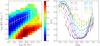 |
Fig. A.1 Same as Fig. 5, but for Sref sample of galaxies. Left panel: Log SFR – Log M⋆ plane colour–coded according to the weighted average B/T in the bin. The white line represents the location of the MS of SFGs, and the error bars show its dispersion. Right panel: B/T ratio as a function of ΔMS (distance from the MS) in different stellar mass bins. |
Appendix B: Concentration in the Log SFR – Log M⋆ plane: R90/R50
We show here the behaviour of the concentration index (R90/R50) in the Log SFR – Log M⋆ plane in the SALL sample. The values of R50 and R90 are taken from the SDSS DR7 catalogues. Figure B.1 shows that the concentration index is minimum on the MS, and it increases both towards larger and smaller SFRs. Bulges in the upper and lower envelopes of the MS are characterised by an average R90/R50 ≈ 2.5 which, according to G09, is the typical concentration index of classical bulges with low values of D4000, which suggests a young age (see Fig. 20 of G09). Classical bulges in the passive region have, on average, a R90/R50 of 3, typical of bulges with high values of D4000 suggesting an old stellar population. Pseudobulges are characterised by R90/R50 ≈ 2.0. We conclude that the upper and lower envelopes of the MS are populated by bulgy galaxies with classical bulges with a relatively young population.
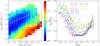 |
Fig. B.1 Left panel: Log SFR – Log M⋆ plane colour–coded as a function of the weighted average of the R90/R50 ratio. The white line represent the location of the MS of SFGs, and the error bars its dispersion. Rightpanel: R90/R50 ratio as a function of the distance from the MS (ΔMS) in different stellar mass bins. |
All Tables
Main sequence SFRs (first column) and dispersion values (second column) in bins of stellar mass, in Log (M/M⊙) (third column).
All Figures
|
Fig. 1 Distribution of galaxies in SALL sample in the Log SFR – Log M⋆ plane. Top panels: SFR distribution of galaxies in three different stellar mass bins. The red solid line is the result of the gaussian fit to the right-side of the SF peak. Bottom panel: Log SFR – Log M⋆ plane colour-coded as a function of the number of galaxies in each bin. The contours encircle bins that host a number of galaxies from 50 to 1250, with step of 250. The MS of SFGs is indicated by the thick solid line, while the error bars mark the 1σ scatter. |
| In the text | |
|
Fig. 2 Completeness in the (g−r) – Log M⋆ plane (left panel) and Log SFR – Log M⋆ plane (right panel) of the spectroscopic SALL sample with respect to the parent photometric Sphot sample. |
| In the text | |
|
Fig. 3 Comparison between B/TBUDDA and B/TGIM2D. The red stars are the median value of the B/TGIM2D in bins of 0.1 B/TBUDDA for all galaxies that the two catalogues have in common, while the blue triangles and black circles are used for the subsamples of barred and unbarred galaxies, respectively. The error bars are given by the standard deviation in each bin. |
| In the text | |
|
Fig. 4 Distribution of the S11 B/T in the different morphological classes defined by Galaxy Zoo 2 (from top to bottom: Sd, Sc, Sb, Sa, and ellipticals). The histograms have been normalised to the peak. The red dashed histograms describe barred spirals, while the black dashed histograms indicate unbarred spirals. The whole population of barred and unbarred galaxies is described by the black solid histograms. |
| In the text | |
|
Fig. 5 Left panel: Log SFR – Log M⋆ plane colour-coded according to the weighted average B/T in the bin. The white line represents the location of the MS of SFGs, and the error bars indicate its dispersion. Right panel: B/T ratio as a function of ΔMS (distance from the MS) in different stellar mass bins. The dotted vertical line indicate the position of the MS. Error bars are obtained via bootstrapping. |
| In the text | |
|
Fig. 6 Fraction of galaxies as a function of the B/T within the MS (black circles), in the upper envelope of the MS (blue stars), in the green valley, and in the passive region (red triangles). The fraction is estimated as the mean in several bin of stellar mass from 1010 to 1011M⊙. The error bars show the dispersion around the mean. The MS upper envelope and the lower envelope (green valley) share the same distribution of galaxies as a function of the B/T: ~40% of the population has B/T > 0.4 vs. 15% of the galaxies in the MS. |
| In the text | |
|
Fig. 7 Left panel: Log SFR – Log M⋆ plane for galaxies in the bulge-disc decomposition catalogue of G09. Each marker is colour-coded accordingly to the B/T value of the galaxy. Right panel: B/T as a function of the distance from the MS, ΔMS, for the G09 whole sample (shaded region), and for the G09 subsample of unbarred galaxies (solid lines). The sample was divided into two bins of stellar mass, 10.0 ≤ Log(M⋆/M⊙) < 10.5 (in black) and 10.5 ≤ Log(M⋆/M⊙) < 11.0 (in red). The B/T distributions computed for the SALL sample are also shown for comparison in dashed lines. The solid vertical lines indicates the location of the MS. error bars are obtained via bootstrapping. |
| In the text | |
|
Fig. 8 Left panel: distribution of galaxies in the Log SFR – Log M⋆ plane, in which each bin (0.2 M⊙ in M⋆ and 0.2 M⊙ yr-1 in SFR) is colour-coded according to the weighted average value of the velocity dispersion σe in the bin. The white line represents the location of the MS of SFGs. Right panel: σe as a function of the distance from the MS, ΔMS, in six different bins of stellar mass, each 0.2 M⊙ wide. The different bins of stellar mass are indicated with different colours, as defined in the legend of the image, while the grey dotted vertical line represents the location of the MS. The error bars are obtained via bootstrapping. |
| In the text | |
|
Fig. 9 Galaxy (left panels), disc (central panels), and bulge (right panels) colours in the Log SFR – Log M⋆ plane. In the upper panels, the distribution of galaxies in the Log SFR – Log M⋆ plane is colour-coded according to the weighted average (g−r) colour in each bin. The bins are 0.2 M⊙ in Log M⋆ and 0.2 M⊙ yr-1 in Log SFR. In the bottom panels, the (g−r) colour is shown as a function of the distance from the MS, ΔMS, in different bins of stellar mass, represented by different colours (same as Fig. 5). The error bars in the lower panels are obtained via a bootstrapping. |
| In the text | |
|
Fig. 10 Balmer decrement in the Log SFR – Log M⋆ plane for galaxies in our sample that have a median S/N per pixel >8. The white solid line and error bars represent the MS of SFGs and its dispersion. |
| In the text | |
|
Fig. 11 B/T ratio, as a function of the distance from the MS, represented by the vertical dotted line. Here ΔMS was computed from the sSFR normalised to Mdisc. Different bins of stellar mass are indicated with different colours. |
| In the text | |
|
Fig. A.1 Same as Fig. 5, but for Sref sample of galaxies. Left panel: Log SFR – Log M⋆ plane colour–coded according to the weighted average B/T in the bin. The white line represents the location of the MS of SFGs, and the error bars show its dispersion. Right panel: B/T ratio as a function of ΔMS (distance from the MS) in different stellar mass bins. |
| In the text | |
|
Fig. B.1 Left panel: Log SFR – Log M⋆ plane colour–coded as a function of the weighted average of the R90/R50 ratio. The white line represent the location of the MS of SFGs, and the error bars its dispersion. Rightpanel: R90/R50 ratio as a function of the distance from the MS (ΔMS) in different stellar mass bins. |
| In the text | |
Current usage metrics show cumulative count of Article Views (full-text article views including HTML views, PDF and ePub downloads, according to the available data) and Abstracts Views on Vision4Press platform.
Data correspond to usage on the plateform after 2015. The current usage metrics is available 48-96 hours after online publication and is updated daily on week days.
Initial download of the metrics may take a while.