| Issue |
A&A
Volume 597, January 2017
|
|
|---|---|---|
| Article Number | A54 | |
| Number of page(s) | 12 | |
| Section | Galactic structure, stellar clusters and populations | |
| DOI | https://doi.org/10.1051/0004-6361/201629051 | |
| Published online | 21 December 2016 | |
The properties of red giant stars along the Sagittarius tidal tails ⋆
1 Shandong Provincial Key Laboratory of Optical Astronomy and Solar-Terrestrial Environment, School of Space Science and Physics, Shandong University at Weihai, 264209 Weihai, PR China
e-mail: This email address is being protected from spambots. You need JavaScript enabled to view it.
2 Key Laboratory of Optical Astronomy, National Astronomical Observatories, Chinese Academy of Sciences, 100012 Beijing, PR China
3 Research School of Astronomy and Astrophysics, The Australian National University, Weston Creek, ACT 2611, Australia
4 University of Chinese Academy of Sciences 19A Yuquan Rd, Shijingshan District, 100049 Beijing, PR China
5 Physics and Geosciences, Angelo State University, San Angelo, TX 76904, USA
6 Nanjing Institute of Astronomical Optics & Technology, National Astronomical Observatories, Chinese Academy of Sciences, 210042 Nanjing, PR China
Received: 3 June 2016
Accepted: 30 September 2016
Abstract
Aims. We aim to measure the metallicity distribution and velocity distribution of red giant branch (RGB) stars along the Sagittarius dwarf galaxy (Sgr) streams. Thanks to the large number of stars of the Sloan Digital Sky Survey (SDSS) sample, we can study the properties of streams as a function of the Λ⊙ from the Sgr core.
Methods. Using the ~22 000 RGB stars from the ninth data release of SDSS, we selected 1100 RGB stars belonging to the streams of the Sgr. As compared with red horizontal branch stars (Shi et al. 2012, ApJ, 751, 130) the RGB stars constitute a large sample size and extend to a metal-poor component of [Fe/H] ~−3.0 dex. In particular, this RGB sample has a significant number of stars in the second wrap of the leading stream of the Sgr (leading arm 2), and thus provides a good opportunity to understand the properties of the leading stream.
Results. We derive a metallicity gradient of −(2.3 ± 0.5) × 10-3 dex deg-1 in leading arm 2 for the first time, of −(1.6 ± 0.4) × 10-6 dex deg-1 for the leading arm 1, and of −(1.3 ± 0.3) × 10-3 dex deg-1 for the trailing arm 1. We check the distribution of Sgr stars in phase space and find a velocity dispersion of ~21.5 km s-1 for leading arm 1. Finally, we identify a possible new branch in leading arm 1.
Key words: stars: abundances / Galaxy: halo / Galaxy: structure
Full Table A.1 is available at the CDS via anonymous ftp to cdsarc.u-strasbg.fr (130.79.128.5) or via http://cdsarc.u-strasbg.fr/viz-bin/qcat?J/A+A/597/A54
© ESO, 2016
1. Introduction
It is well established that the Galaxy has gained an important fraction of its mass through tidal destruction and accretion of a large number of low-mass satellite galaxies. A growing number of observations point out that the Sagittarius dwarf galaxy (Sgr) is disrupting into the Milky Way and is becoming the building blocks of the Galaxy. Therefore, studying the metallicity and kinematics of Sgr can help us understand the formation of the Galaxy and the process of how the Galaxy accretes its satellite galaxies (Chen et al. 2014; Hyde et al. 2015; Carlin et al. 2012; de Boer et al. 2015; Eggen et al. 1962; Searle & Zinn 1978; White & Frenk 1991; Johnston et al. 2008).
The Sgr is stretched out along two giant tidal streams, that is, a leading stream and trailing stream, under the strain of the Galaxy. Many works on the trailing and leading stream of Sgr have been done. Hyde et al. (2015) identified 106 members of the Sgr streams and found a metallicity distribution ranging from –0.59 dex to –0.97 dex over 142 deg in the Sgr trailing stream. De Boer et al. (2014) analyzed the α-element distribution of the stellar members of the Sgr trailing stream and found that the α-element distribution of the Sgr trailing stream was forming a narrow sequence at intermediate metallicities with a clear turn-down, which is consistent with the presence of an α-element knee. Koposov et al. (2015) used the M giants to trace the Sgr trailing tail behind the Galactic disk in the direction of the anti-centre, and they provided a new kinematic detection of the Sgr trailing tail debris at Λ⊙ = 204°. Carrell et al. (2012) probed a section of the trailing stream of the Sgr and determined an absolute stellar density of 2.7 ± 0.5 red clump (RC) stars kpc-3. Belokurov et al. (2014) showed that the globular cluster NGC 2419 could be associated with the Sgr trailing arm based on the position and radial velocity. Bellazzini et al. (2006) found a gradient describing the ratio of old stars to young stars along the arms of the Sgr and found the ratio of the blue horizontal branch (BHB) stars to RC stars to be five times larger in the leading arm than in the core of the dwarf galaxy. Yanny et al. (2009) showed that the ratios of K/M giants to BHBs and BHBs to F-turnoff stars are similar for two branches of the leading stream and found a metallicity gradient of −0.8 ± 0.2 dex deg-1 for 33 identified Sgr K/M-giant stars, as measured by the seventh data release of the Sloan Digital Sky Survey (SDSS DR7). Most works focus on the trailing stream, while few analyses have been carried out for the leading stream.
Shi et al. (2012) selected red horizontal branch (RHB) stars along the streams of the Sgr from SDSS DR7 spectroscopic data with the help of the Law & Majewski (2010) model. The model is based on observational data from 2MASS and SDSS, and it divides the 105 points into four parts: leading arm 1, leading arm 2, trailing arm 1, and trailing arm 2. Shi et al. (2012) selected 102, 78, 327, and 31 RHB stars in leading arm 1, leading arm 2, trailing arm 1, and trailing arm 2 respectively. The largest number of member stars are located in trailing arm 1, so the analysis of this region is reasonable and the results are robust. However, the results for leading arms are somewhat limited by the small sample, and we need a larger sample to further study the leading stream of the Sgr.
The SDSS survey provides a huge number of red giant branch (RGB) stars, from which we could obtain more member stars of Sgr streams, especially in the leading stream. In this work, we present the general properties of Sgr streams based on the RGB stars from the SDSS DR9 database, in which the spectroscopic data provides stellar parameters, that is, distances, radial velocities, and metallicities for stars extending over a wide area. The paper is organised as follows: in Sect. 2, we present the method used to select the Sgr sample. In Sect. 3, the results and properties of streams are analysed. In Sect. 4, the error analysis is discussed. Finally, a summary is given in Sect. 5.
2. Sample selection
2.1. Ra-Dec and distance selection
We obtained ~22 000 RGB stars from SDSS DR9 low resolution spectral data (Chen et al. 2014). Tan et al. (2014) determined distances for RGB stars with two methods. The first method follows Xue et al. (2014) and the second method follows the procedures adopted in Kordopatis et al. (2011). Both methods give similar results for most stars, but have large deviations for some stars. The large deviation comes from the inclusion of spectroscopic Teff and log g as additional input parameters in the second method.
Following Chen et al. (2014), we removed those stars which had a large error in distance. We selected stars with a difference in distance that is less than 30% between the two methods, and stars with an error that is less than 30% in each method. Finally, we obtained 16490 stars with accurate parameters.
We selected Sgr member stars by using the Law & Majewski (2010) model which provided a model of the Sgr orbiting in a triaxial Galactic potential, as above mentioned. The procedure we used to select our Sgr sample is similiar to that of Shi et al. (2012).
-
(1)
We selected a sample along the directions of Sgr streams in anRa-Dec map and obtained 8332 stars.
-
(2)
We used distance to choose the candidates that were located at the position of the Sgr streams in a Λ⊙-Distance map. Here, Λ⊙ is the Sgr longitude scale along the orbital plane. We obtained 1343, 1374, 1118, and 478 stars in leading arm 1, leading arm 2, trailing arm 1 and trailing arm 2, respectively. The stars with the distance criteria are shown with blue dots in trailing arm 1 and red dots in leading arm 1 in Fig. 1. For the other sections of the stream, details can be found in Fig. 1 of Shi et al. (2012).
-
(3)
We selected sample stars using a Λ⊙-Vgsr map, which will be described in detail in Sect. 2.2.
2.2. Vgsr selection and the new boundary
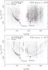 |
Fig. 1 Λ⊙ vs. Vgsr diagram for RGB and RHB stars. Upper panel: the dots are ~22 000 RGB stars from SDSS DR9. The red dashed lines indicate the boundaries of the Law & Majewski (2010) model. The upper boundary of trailing arm is fitted in this work and shown by a solid line. The blue dotted and dashed lines are provided by Yanny et al. (2009). The stars with the distance cuts are shown with blue dots for the trailing stream and red dots for the leading stream. Leading arm and trailing arm are also labelled. Lower panel: same as upper panel but for 8535 RHB stars. |
We used the Vgsr (radial velocity in the Galactic standard of rest) to choose the member stars of the Sgr streams in a Λ⊙-Vgsr map (Fig. 1 in Shi et al. 2012). We calculated the Vgsr with the same equation as Shi et al. (2012), that is, Vgsr = rv + 9.0cosbcosl + 232.0cosbsinl + 7.0sinb km s-1. Figure 1 shows the RGB stars database in the Λ⊙-Vgsr map, in which we can clearly see a dense band (60°< Λ⊙< 130°) in the left half of the panel, corresponding to the main body of trailing arm 1. We fit the high boundary of this part (60°< Λ⊙< 130°) of trailing arm 1:  , which is shown with a solid line in Fig. 1. The low boundary is provided by the Law & Majewski (2010) model:
  . The selection criteria of the Sgr sample is flow(x) < Vgsr < fhigh(x). We also can distinguish the main body of leading arm 1 from the DR9 database. The selection criteria of the part (180°< Λ⊙ < 320°) of leading arm 1 follows the method used in Yanny et al. (2009) and Chen et al. (2014): flow(x) < Vgsr < fhigh(x) where
  and fhigh(x) = 0.017 ∗ (Λ⊙−200.0)2−80.0. We found that the dense band of the RGB stars agrees well with these boundaries in the upper panel of Fig. 1. As for other parts (other parts of leading arm 1, other parts of trailing arm 1, leading arm 2, and trailing arm 2), we chose the sample using the Law & Majewski (2010) model (as in Fig. 1 in Shi et al. 2012). Excluding overlapping stars, we finally got 441 and 321 stars belonging to leading arms 1 and 2, respectively, and 308 and 30 stars belonging to trailing arms 1 and 2, respectively.
We used the 8535 RHB stars from SDSS DR7 (Shi et al. 2012 and Chen et al. 2010) to verify the new boundary in trailing arm 1. We plotted these RHB stars in the Λ⊙-Vgsr map in the lower panel of Fig. 1. From this map, we found that the dense band of RHB stars falls well within the new boundary. It seems that the RHB stars agree well with the new boundary of the RGB stars, especially at 60° < Λ⊙ < 130°. This indicates that the new boundary is reasonable.
The first ten RGB stars of the Sgr streams are listed in Table A.1 and the whole table of our Sgr sample is provided in an electronic version at the CDS. In Table A.1, the following parameters are listed: star identification, right ascension, declination, [Fe/H], distance, Vgsr, Λ⊙, XGC, YGC, ZGC , and mark (T1, T2, L1, and L2 mean trailing arm 1, trailing arm 2, leading arm 1, and leading arm 2, respectively).
3. Results
3.1. Comparing the properties of the RGB and RHB samples
RGB and RHB stars are two important tracers used to detect the Sgr streams. RHB stars have nearly constant absolute magnitude so that they constitute an ideal sample to trace various Galactic populations and Sgr streams. RGB stars are main populations and thus the sample size can be large and can therefore produce good statistics.
3.1.1. Locations and the number of member stars
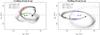 |
Fig. 2 Position of programme stars in the Cartesian galactocentric plane. The black points represent the leading and trailing streams in the model by Law & Majewski (2010). Left panel: red stars show RGB stars in leading arm 1 and green stars show RGB stars in leading arm 2. The Galactic plane (dashed line), the position of the Sun, and the Galactic centre are also marked for reference. The blue box and the dashed line will be described in Sect. 3.4.2. Right panel: RGB stars in the trailing stream. Blue stars show RGB stars in trailing arm 1 and pink stars show RGB stars in trailing arm 2. We kept consistent colour for the given structures throughout the manuscript. |
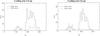 |
Fig. 3 Comparing the number of the RGB sample and the RHB sample in the leading stream along the Sgr longitude scale. Solid lines represent the RGB stars and dashed lines show the RHB stars. |
The X-Z distribution of RGB stars in the Sgr streams is shown in Fig. 2. Comparing with the RHB stars shown in Fig. 2 of Shi et al. (2012), we can see that our RGB sample has a roughly similar location distribution as the RHB sample in Shi et al. (2012), but our RGB sample covers a wider region especially in the leading stream. From Fig. 3, we can see that the number of stars in our RGB sample is clearly larger than that of the RHB sample in the leading arms. The RHB stars are the Sgr sample provided by Table A.1 of Shi et al. (2012). A wider region and a larger number are the advantages of the RGB stars and are propitious for us to obtain more credible results.
3.1.2. Metallicity distribution
For comparison, we plot the histograms of [Fe/H] for RGB and RHB stars in Fig. 4. For the large number and high density, we compare two parts: 180°< Λ⊙< 320° of leading arm 1 (there are 397 RGB stars and 77 RHB stars) and 60°< Λ⊙< 130° of trailing arm 1 (there are 194 RGB stars and 271 RHB stars). In the data for leading arm 1 shown in Fig. 4, the metallicity peak of the RHB stars is at [Fe/H] ~−1.2 dex and the [Fe/H] extend to ~–1.6 dex, while the metallicity peak of the RGB stars is at [Fe/H] ~−1.4 dex and the [Fe/H] of the RGB stars extends to a metal-poorer [Fe/H] ~−3.0. In the data for trailing arm 1, shown in Fig. 4, the metallicity peaks of the RHB stars are at [Fe/H] ~−1.2 dex and ~–0.8 dex with no RHB stars more metal poor than ~–1.7 dex. The metallicity peak of the RGB stars is at [Fe/H] ~−1.3 dex and there are metal poor stars down to [Fe/H] ~−2.7 dex. The [Fe/H]-distribution of the RGB sample has a wide range, that is, the RGB stars not only include the metal-rich component but also the metal-poor component of the Sgr streams.
3.2. The metallicity gradient
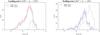 |
Fig. 4 Comparison of [Fe/H] distribution of RGB and RHB stars in Sgr streams. The solid lines represent the RGB stars and the dashed lines show the RHB stars. The Poisson errors are added in the histograms of RGB stars. |
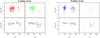 |
Fig. 5 [Fe/H] of RGB stars as a function of angular distance from Sgr core along the leading stream (left panels) and trailing stream (right panels). The upper panels show the individual RGB stars. In the lower panels, the distribution of [Fe/H] is displayed as the median. The solid line shows the result of a least-squares linear fit to the median data of RGB stars. |
In order to confirm or deny the existence of a metallicity gradient in our sample along the Sgr leading and trailing tidal streams, we investigated the [Fe/H] distribution of RGB stars as a function of orbital longitude along the streams. In Fig. 5, the upper panels show the individual points of the RGB stars, the lower panels present the median of the individual points with a bin size of 20 deg. The solid lines show the result of a least-squares linear fit to the median data. We find a metallicity gradient of −(1.6 ± 0.4) × 10-6 dex deg-1 in leading arm 1, of −(2.3 ± 0.5) × 10-3 dex deg-1 in leading arm 2 and of −(1.3 ± 0.3) × 10-3 dex deg-1 in trailing arm 1. Stars in trailing arm 2 are so sparse that we cannot obtain the metallicity gradient and only present the median points in the map.
Clearly, there is a negative gradient in trailing arm 1. Our results agree well with the gradient found by Chou et al. (2007), Shi et al. (2012), Hyde et al. (2015), Keller et al. (2010), and Yanny et al. (2009) and are similar to Fig. 15 of Law & Majewski (2010) which gives the distribution of [Fe/H]. We find a negative gradient in leading arm 2 for the first time due to the large number of RGB stars and an ideal distribution of the median data. The negative gradient is coincident with the dwarf-galaxy formation theory that the older the star is, the farther away from the core and the more metal-poor it is. That is to say, the outer, older, and metal-poor population is tidally stripped before the inner, younger, metal-rich component. The Law & Majewski (2010) model shows the trailing arm from core to tail corresponding to Λ⊙ from 0° to 360°, while leading arm corresponding to Λ⊙ from 360° to 0° (see Fig. 5).
However, we find a slightly flat gradient in leading arm 1. Our result is similiar to that of Hyde et al. (2015) who also lack a clear gradient because of high metallicity dispersion. The possible reasons for this are that the RGB stars include a metal poor component in the high-Λ⊙ part (180° < Λ⊙ < 320°), so the metallicity of the high-Λ⊙ part is low. The sample number of the low-Λ⊙ part (60°< Λ⊙< 150°) of leading arm 1 is not enough, especially for stars more metal poor than [Fe/H] ~−2.0 dex.
We narrowed the boundaries by 10 km s-1 for the sample selection in the Λ⊙-Vgsr map of the high-Λ⊙ part of leading arm 1. We recalculated the gradient with the boundary flow(x) < Vgsr < fhigh(x) where  and fhigh(x) = 0.017 ∗ (Λ⊙−200.0)2−90.0. The result is still nearly flat. So we consider the boundary of Yanny et al. (2009) to be reliable and our results are robust.
3.3. Velocity distribution
3.3.1. Velocity distribution in phase space
From Fig. 6, we can see that the nearest stars to us is the part covering 180° < Λ⊙ < 320° of the leading arm 2, which is nearly ~9 kpc. The stars in trailing arm 1 present a symmetrical continuous distribution and cross with leading arm 1 at ~25 kpc. The stars in trailing arm 2 are rare so we do not analyse them in detail. The stars in leading arm 1 are located at a wide range in distance, from 10 kpc to 60 kpc. These stars present a linear distribution, which is fitted by a polynomial and shown with a black solid line in Fig. 6. The solid line describes a characteristic trend of increasing Vgsr with increasing distance. The velocity residuals of our sample stars, along with the polynomial fit and the gaussian fit of velocity residual, are shown in Fig. 7. The value of velocity dispersion in leading arm 1 is 21.5 ± 2.2 km s-1 with 397 RGB stars.
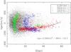 |
Fig. 6 Distance vs. Vgsr diagram for Sgr RGB stars. The dots represent all ~22 000 RGB stars, green circles show stars in leading arm 2, red circles show stars in leading arm 1, blue circles show stars in trailing arm 1, and pink circles show stars in trailing arm 2. The black solid line shows the polynomical fit of the RGB stars in the part (180° < Λ⊙ < 320°) of leading arm 1. |
3.3.2. Velocity distribution in Λ⊙−Vgsr map
We also plotted those stars in the part 180°< Λ⊙< 320° of leading arm 1 in a Λ⊙−Vgsr map, fitted them with a polynomial, and calculated the velocity dispersion of those stars in the Λ⊙−Vgsr map. The velocity dispersion is σL = 19.4 ± 1.9 km s-1.
We recalculated the velocity dispersion in Λ⊙−Vgsr space of trailing arm 1 (60°< Λ⊙ < 130°) and obtained σT = 13.9 ± 1.4 km s-1. Monaco et al. (2007) gave a velocity dispersion of σ = 8.3 ± 0.9 km s-1 using 41 stars with high resolution spectroscopy, and Majewski et al. (2004) gave σ = 10.4 ± 1.3 km s-1 for stars with low resolution spectroscopy. Shi et al. (2012) gave σ = 9.8 ± 1.0 km s-1 with 119 RHB stars. These values are consistent within errors.
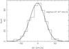 |
Fig. 7 Gaussian fit of velocity residual of the RGB stars in leading arm 1 (180°< Λ⊙ < 320°) in phase space. |
3.4. A possible new branch in Sgr tidal tails
We were able to detect more than one peak in the density profiles of the streams, which indicates an intricate structure and multiple branches of the tidal debris.
3.4.1. Spectral confirmation for a known branch
Koposov et al. (2012, K12) suggest that the debris of the Sgr trailing arm in the south (90° < Λ⊙ < 120°) is actually two branches of stars separated by ~10° in the Sgr orbital coordinate system based on the main sequence turn-off (MSTO) and M giant stars. We selected 144 candidates from 90° < Λ⊙ < 120° in the trailing arm, which are shown as the dashed line in the histogram in Fig. 8, where we can see four peaks at B⊙ ~ 9°, B⊙ ~ 3°, B⊙ ~ −2°, and B⊙ ~ −7°. Then we selected bright and faint branches with the criteria which K12 provided, and obtained 59 RGB stars in the bright branch and 5 RGB stars in the faint branch from 144 RGB trailing stars. We plot them in Fig. 8, and we can clearly see the position of the bright and faint branches. The blue solid line indicates that the weak peak at B⊙ ~ 9° is the faint branch found by K12. Therefore, we confirm the photometric detection of two branches by K12 based on the spectral database of RGB stars. We also detect three other peaks in the bright stream.
3.4.2. Identification of a possible new branch
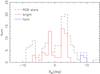 |
Fig. 8 Across-stream profiles of RGB stars in 90° < Λ⊙ < 120° of the trailing arm. Red solid line is the bright branch selected with the criteria which Koposov et al. (2012) provided. The blue solid line is the faint branch selected with the criteria which Koposov et al. (2012) provided. The dashed line is all the RGB stars in 90° < Λ⊙ < 120° of the trailing arm. |
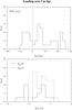 |
Fig. 9 Upper panel: across-stream profiles of leading arm 1 (60° < Λ⊙ < 160°) with RGB stars. Lower panel: distribution of [Fe/H] of main stream (B⊙ > 0°) and the branch (B⊙ < 0°). The solid line shows the stars of the branch and the dashed line show the stars of the main stream. |
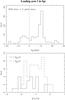 |
Fig. 10 Upper panel: across-stream profiles of leading arm 1 with RGB stars and K giant stars. Lower panel: distribution of [Fe/H] of main stream and branch, the solid line shows the branch and the dashed line shows the main stream. |
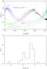 |
Fig. 11 Upper panel: Λ⊙ vs. D diagram for Sgr streams and the Virgo over-density (VOD). The dots are from the Law & Majewski (2010) model. Trailing arm 1 and leading arm 2 are marked with blue and green, respectively. Red triangles show the VOD. We can see that the VOD is very near to the streams of Sgr. Lower panel: [Fe/H] distribution of 36 stars in the VOD. |
Confirmation of the branches found by K12 gives us confidence to look for other possible sub-components of the tidal streams in our dataset.
We detected a possible branch in the leading arm 1 in the south (60°< Λ⊙< 160°). We took 44 RGB stars from our sample in this part and plotted them in Fig. 9, where we can see two main peaks at ~−5° and ~ 6°, respectively. We divided leading arm 1 into two groups, B⊙ > 0° and B⊙ < 0°. We compared the [Fe/H] of these two groups of stars in the lower panel of Fig. 9. We can see two components ([Fe/H] < −2.0, [Fe/H] > −2.0) in the part of B⊙ < 0°, while only one component in B⊙ > 0°. The stars of B⊙ < 0° have different metallicities and possibly comprise a new branch in leading arm 1.
For further confirmation, we selected Sgr member-stars in this same position (60°< Λ⊙ < 160° of leading arm 1) from K giant stars of the first data release of the Large Sky Area Multi-Object Fiber Spectroscopic Telescope (LAMOST DR1; Liu et al. 2014) with our selection-method mentioned above and obtained 95 K giants. We plot RGB stars and K giant stars together in Fig. 10, where we can see two peaks at ~−5° and ~ 10°, respectively. We suspect the peak at ~ 10° is the main stream and the weak peak at ~−5° is the branch. We divided stars in the leading arm 1 into two groups, B⊙ > 0° and B⊙ < 0°. We compare [Fe/H] of these two parts in the lower panel of Fig. 10 (excluding 58 stars that do not have [Fe/H] values from LAMOST). We can see that the B⊙ < 0° part has a metal-poor component, while the B⊙ > 0° part does not. Therefore, we suspect that the B⊙ < 0° part is a possible new branch in leading arm 1. We also did the Kolmogorov-Smirnov test (KS test) on the new branch and the main stream and obtained a value ~0.10, which indicates that the branch is likely to be an independent structure.
Belokurov et al. (2006) found one bifurcation in the north leading stream and we detected a possible new branch in the south leading stream. The bifurcation is near our, and could be the same as our branch. In the left panel of Fig. 2, the position of our new branch is marked with a box. We suspect the branches may belong to one continuous stream accompanying the main body of leading arm 1. The possible stream is shown with a blue dashed line, where it is most likely to have a sub-component deduced from the distribution of the Sgr model in the X-Z map (Fig. 2). More observations are needed to confirm this speculation (the forthcoming data from Gaia will probably play a key role, Gaia Collaboration 2016). This possible stream could be very helpful in constraining the substructure of the Sgr tidal debris and the Galactic potential in which it orbits.
3.5. Substructures near the Sgr streams
There are many substructures and clusters near the Sgr streams. One of the most famous is the Virgo over-density (VOD). Chen et al. (2014) summarise the selection criteria from the literature (Duffau et al. 2006, 2010; Newberg et al. 2007; Vivas et al. 2008; Prior et al. 2009; Casey et al. 2012). We used the selection criteria and obtained 36 RGB stars which belong to the VOD. The VOD is close to the streams of Sgr (their position distribution is shown in Fig. 11). As mentioned above, our RGB sample is somewhat metal-poor. To detect the metal-poor component in VOD, we show the [Fe/H] distribution of VOD in Fig. 11. There are two peaks at ~–1.3 and ~–1.9, respectively. As expected, most of the stars are metal-poor.
There are some substructures in VOD such as S297+63-20.5, the Virgo stellar stream (VSS), and a relatively high-velocity substructure. These substructures have different features in velocity and [Fe/H]. We will describe their features and how they are related to the Sgr streams in a paper currently in preparation.
4. Discussion
4.1. The contamination of Galactic halo stars
In this part, we discuss the contamination of Galactic stars in our Sgr sample. To verify the flat metallicity in leading arm 1, we chose the member-stars in 180° < Λ⊙ < 320° of leading arm 1 with Vgsr < −90 km s-1, which is the characteristic velocity of high-probability member stars in Sgr streams following Shi et al. (2012; see Figs. 3–5 in Shi et al. 2012). Then we recalculated the metallicity gradient with these stars to analyse the effect of the Galactic stars. We found that the metallicity gradient also presents a flat trend as above mentioned, which indicates that our result is reasonable in leading arm 1.
We assess contamination from the Galactic stars after the distance cut in velocity space and show these stars with a different colour dots in Fig. 1. In Fig. 1, there is a clear, dense band in trailing arm 1. We estimated the average background of halo stars by counting the stars out of the dense band and calculated that there are 20 halo stars in the trailing stream. Therefore the contamination ratio is nearly 10%, 20 out of 194 member stars, in trailing arm 1. In the same way, the contamination is nearly 25% in the leading stream. These contaminations may have a small effect on the metallicity gradients, but the effect is within the errors on the metallicity gradients.
Furthermore, we analysed the contamination of the Galactic stars as Shi et al. (2012) did. They estimated the contamination of the RHB sample and confirmed that their results are robust. We estimated the level of contamination of our sample from halo RGB stars. We downloaded the Besançon model of the Galaxy (Robin et al. 2003), selected RGB stars from the Besançon model (as Chen et al. 2014 did), and selected Sgr member-stars with the three-step selection criteria mentioned above. Finally we found that the contamination from the Besançon model stars is small and within the error of our results. The halo contamination is also very small according to previous works suffering the same problem (such as Yanny et al. 2009; Monaco et al. 2007; Keller et al. 2010; Correnti et al. 2010; Carrell et al. 2012; Koposov et al. 2012; Shi et al. 2012; Hyde et al. 2015).
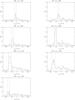 |
Fig. 12 Vgsr distribution of RGB stars for 60° < Λ⊙ < 130° of trailing arm 1. Each panel shows the stars in one 10°-bin. The dashed lines show the boundaries of trailing arm 1. The dotted lines are the fitted distribution of Galactic stars. |
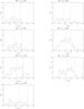 |
Fig. 13 Distance distribution of RGB stars (which are within the dashed lines in Fig. 12) for 60° < Λ⊙ < 130° of trailing arm 1. Each panel shows the stars in one 10°-bin. The dashed lines show the boundaries of trailing arm 1 in distance. |
4.2. Comparing our sample with the star counting method in the trailing arm
We reselected stars of trailing arm 1 in the velocity space with the star counting method. We can clearly see the dense band of trailing arm 1 in the upper panel of Fig. 1, which consists of Sgr trailing-arm stars and Galactic-halo stars (foreground and background stars). We divided trailing-arm stars, which have been selected with Ra-Dec, into seven bins from Λ⊙ = 60° to Λ⊙ = 130°, and we counted the stars in Vgsr bins (see Fig. 12). In each panel of Fig. 12, we can clearly see a peak where the trailing arm goes through. The dashed lines are used to confirm the boundaries of the trailing arm. We get a total of 496 stars between the dashed lines in the seven bins. The dotted line indicates the fitted distribution of Galactic-halo stars, normalised to the number of stars in each range of Λ⊙. We fitted the Galactic stars with dotted lines so that we get a smooth distribution of Galactic stars. Stars between the dashed lines and under the dotted line are Galactic stars, which are roughly 109 in total. The number of stars between the dashed lines minus the number of Galactic stars leaves us with a total of ~387 stars belonging to the trailing arm.
We obtained 194 Sgr stars in the trailing arm (60°< Λ⊙< 130°) with our selection method, as mentioned in Sects. 2.1 and 2.2. The number of stars from the counting method is larger than the number of stars from our method. There are two reasons for this discrepancy. Firstly, the selection does not adopt the distance criterion in the counting method, so the stars with an incorrect distance may be included in the Sgr sample. Secondly, the number of Galactic stars may be underestimated in the counting method.
In Fig. 13, the distance distribution of the 496 RGB stars is shown and the dashed lines show the boundaries of trailing arm 1 in distance. A large fraction of stars are outside the trailing arm range, especially in the foreground. This indicates that some stars with inappropriate distances are counted and Galactic stars are underestimated in the counting method. We obtain 202 member-stars after the distance cut in Fig. 13, which is similar to the 194 stars from our sample selection. This indicates that the distance cut is important.
5. Conclusions
We obtained a large sample of RGB stars from the SDSS DR9 database. The RGB sample was used to confirm the boundaries of the leading arm and the trailing arm of the Sgr tidal streams. Excluding stars with large distance error, which influences the accuracy of [Fe/H], we chose a sample belonging to Sgr through three steps: (1) Ra-Dec (2) Λ⊙-Distance (3) Λ⊙-Vgsr. We finally obtained 441 RGB stars belonging to leading arm 1, 321 stars belonging to leading arm 2, 308 stars belonging to trailing arm 1, and 30 stars belonging to trailing arm 2. Based on the statistical analysis of this sample, five main results are obtained as follows:
-
1.
We give a new boundary
(60°< Λ⊙< 130°) of the trailing arm using a high densityband in the large dataset in velocity space. This is helpful toconstrain the Sgr models. -
2.
The metallicity gradient of RGB stars is −(1.6 ± 0.4) × 10-6 dex deg-1 in leading arm 1, −(2.3 ± 0.5) × 10-3 dex deg-1 in leading arm 2, and −(1.3 ± 0.3) × 10-3 dex deg-1 in trailing arm 1.
-
3.
We fit the velocity along the stream in phase space and calculate a velocity dispersion of 21.5 km s-1 for leading arm 1. Furthermore we recalculated the velocity dispersions along Sgr longitude of leading arm 1 and trailing arm 1, which are σL = 19.4 ± 1.9 km s-1 and σT = 13.9 ± 1.4 km s-1, respectively.
-
4.
We confirm a known branch in trailing arm 1 and give evidence for a possible new branch in leading arm 1 according to their position and [Fe/H] distribution.
-
5.
There are two peaks at ~–1.3 and ~–1.9 in the metallicity distribution of RGB stars in the VOD.
With the LAMOST (Cui et al. 2012; Luo et al. 2012; Zhao et al. 2012; Wang et al. 1996; Su et al. 2004) and the upcoming Gaia spectroscopic survey (Gaia Collaboration 2016), we can expect to analyse stars in the Sgr streams for an even larger sample in order to further study the intricacies of the Sgr galaxy.
Acknowledgments
We thank the referee for his helpful comments which significantly improved the paper. We thank Michael Ireland and XiangXiang Xue for their helpful discussion. This work was supported by the NSFC grant Nos. U1631105, 11390371, 11573035, 11233004, U1331104, 11625313, 11273026 and 11373026, the 973 program No. 2014CB845700 and the Strategic Priority Research Program of the Chinese Academy of Sciences grant No. XDB01020300. Guoshoujing Telescope (the Large Sky Area Multi-Object Fiber Spectroscopic Telescope LAMOST) is a National Major Scientific Project built by the Chinese Academy of Sciences. Funding for the project has been provided by the National Development and Reform Commission. LAMOST is operated and managed by the National Astronomical Observatories, Chinese Academy of Sciences.
References
- Bellazzini, M., Newberg, H. J., Correnti, M., et al. 2006, A&A, 457, L21 [NASA ADS] [CrossRef] [EDP Sciences] [Google Scholar]
- Belokurov, V., Zucker, D. B., Evans, N. W., et al. 2006, ApJ, 642, 137 [Google Scholar]
- Belokurov, V., Koposov, S. E., Evans, N. W., et al. 2014, MNRAS, 437, 114 [Google Scholar]
- Carlin, J. L., Majewski, S. R., Casetti-Dinescu, D. I., et al. 2012, ApJ, 744, 25 [NASA ADS] [CrossRef] [Google Scholar]
- Carrell, K., Wilhelm, R., & Chen, Y. Q. 2012, AJ, 144, 18 [NASA ADS] [CrossRef] [Google Scholar]
- Casey, A. R., Keller, S. C., & Da Costa, G. 2012, AJ, 143, 88 [NASA ADS] [CrossRef] [Google Scholar]
- Chen, Y. Q., Zhao, G., Zhao, J. Z., et al. 2010, AJ, 140, 500 [NASA ADS] [CrossRef] [Google Scholar]
- Chen, Y. Q., Zhao, G., Carrell, K., et al. 2014, ApJ, 795, 52 [NASA ADS] [CrossRef] [Google Scholar]
- Chou, M. Y., Majewski, S. R., Cunha, K., et al. 2007, ApJ, 670, 346 [NASA ADS] [CrossRef] [Google Scholar]
- Correnti, M., Bellazzini, M., Ibata, R. A., et al. 2010, ApJ, 721, 329 [NASA ADS] [CrossRef] [Google Scholar]
- Cui, X. Q., Zhao, Y. H., Chu, Y. Q., et al. 2012, RA&A, 12, 1197 [Google Scholar]
- de Boer, T. J. L., Belokurov, V., Beers, T. C., & Lee, Y. S. 2014, MNRAS, 443, 658 [NASA ADS] [CrossRef] [Google Scholar]
- de Boer, T. J. L., Belokurov, V., & Koposov, S. 2015, MNRAS, 451, 3489 [NASA ADS] [CrossRef] [Google Scholar]
- Duffau, S. V., Zinn, R., Carraro, G., et al. 2006,ApJ, 636, 97 [Google Scholar]
- Duffau, S., Vivas, A. K., Zinn, R., Méndez, R. A., & Ruiz, M. T. 2010, in Stellar Populations: Planning for the Next Decade, eds. G. Bruzual, & S. Charlot (Cambridge: Cambridge Univ. Press), IAU Symp., 262, 131 [Google Scholar]
- Eggen, O. J., Lynden-Bell, D., & Sandage, A. R. 1962, ApJ, 136, 748 [NASA ADS] [CrossRef] [Google Scholar]
- Gaia Collaboration (Brown, A. G. A., et al.) 2016, A&A, 595, A2 [NASA ADS] [CrossRef] [EDP Sciences] [Google Scholar]
- Hyde, E. A., Keller, S., Zucker, D. B., et al. 2015, ApJ, 805, 189 [NASA ADS] [CrossRef] [Google Scholar]
- Johnston, K. V., Bullock, J. S., Sharma, S., et al. 2008, ApJ, 689, 936 [NASA ADS] [CrossRef] [Google Scholar]
- Keller, S. C., Yong, D., & Da Costa, G. S. 2010, ApJ, 720, 940 [NASA ADS] [CrossRef] [Google Scholar]
- Koposov, S. E., Belokurov, V., Evans, N. W., et al. 2012, ApJ, 750, 80 [NASA ADS] [CrossRef] [Google Scholar]
- Koposov, S. E., Belokurov, V., Zucker, D. B., et al. 2015, MNRAS, 446, 3110 [NASA ADS] [CrossRef] [Google Scholar]
- Kordopatis, G., Recio-Blanco, A., de Laverny, P., et al. 2011, A&A, 535, A170 [Google Scholar]
- Law, D., & Majewski, S. 2010, ApJ, 714, 229 [NASA ADS] [CrossRef] [Google Scholar]
- Liu, C., Deng, L. C., Carlin, J. L., et al. 2014, ApJ, 790, 110 [NASA ADS] [CrossRef] [Google Scholar]
- Luo, A. L., Zhang, H. T., Zhao, Y. H., et al. 2012, RA&A, 12, 1243 [Google Scholar]
- Majewski, S. R., Kunkel, W. E., Law, D. R., et al. 2004, AJ, 128, 245 [Google Scholar]
- Monaco, L., Bellazzini, M., Bonifacio, P., et al. 2007, A&A, 464, 201 [NASA ADS] [CrossRef] [EDP Sciences] [Google Scholar]
- Newberg, H. J., Yanny, B., Cole, N., et al. 2007, ApJ, 668, 221 [NASA ADS] [CrossRef] [Google Scholar]
- Prior, S. L., Da Costa, G. S., & Murphy, S. J. 2009, ApJ, 691, 306 [NASA ADS] [CrossRef] [Google Scholar]
- Robin, A. C., Reylé, C., Derrière, S., & Picaud, S. 2003, A&A, 409, 523 [NASA ADS] [CrossRef] [EDP Sciences] [Google Scholar]
- Searle, L., & Zinn, R. 1978, ApJ, 225, 357 [NASA ADS] [CrossRef] [Google Scholar]
- Shi, W. B., Chen, Y. Q., Carrell, K., & Zhao, G. 2012, ApJ, 751, 130 [NASA ADS] [CrossRef] [Google Scholar]
- Su, D. Q., & Cui, X. Q. 2004,Chin. J. Astron. Astrophys., 4, 1 [Google Scholar]
- Tan, K. F., Chen, Y. Q., Zhao, J. K., et al. 2014, ApJ, 794, 60 [NASA ADS] [CrossRef] [Google Scholar]
- Vivas, A. K., Jaffe, Y. L., & Zinn, R. 2008, AJ, 136, 164 [NASA ADS] [CrossRef] [Google Scholar]
- Wang, S. G., Su, D. Q., Chu, Y. Q., et al. 1996, Appl. Opt., 25, 5155 [NASA ADS] [CrossRef] [PubMed] [Google Scholar]
- White, S. D. M., & Frenk, C. S. 1991, ApJ, 379, 52 [NASA ADS] [CrossRef] [Google Scholar]
- Xue, X. X., Ma, Z. B., Rix, H. W., et al. 2014, ApJ, 784, 170 [NASA ADS] [CrossRef] [Google Scholar]
- Yanny, B., Newberg, H. J., Johnson, J. A., et al. 2009, ApJ, 700, 1282 [NASA ADS] [CrossRef] [Google Scholar]
- Zhao, G., Zhao, Y. H., Chu, Y. Q., et al. 2012, RA&A, 12, 723 [Google Scholar]
Appendix A: Additional table
List of 1100 RGB stars in Sgr streams.
All Tables
All Figures
|
Fig. 1 Λ⊙ vs. Vgsr diagram for RGB and RHB stars. Upper panel: the dots are ~22 000 RGB stars from SDSS DR9. The red dashed lines indicate the boundaries of the Law & Majewski (2010) model. The upper boundary of trailing arm is fitted in this work and shown by a solid line. The blue dotted and dashed lines are provided by Yanny et al. (2009). The stars with the distance cuts are shown with blue dots for the trailing stream and red dots for the leading stream. Leading arm and trailing arm are also labelled. Lower panel: same as upper panel but for 8535 RHB stars. |
| In the text | |
|
Fig. 2 Position of programme stars in the Cartesian galactocentric plane. The black points represent the leading and trailing streams in the model by Law & Majewski (2010). Left panel: red stars show RGB stars in leading arm 1 and green stars show RGB stars in leading arm 2. The Galactic plane (dashed line), the position of the Sun, and the Galactic centre are also marked for reference. The blue box and the dashed line will be described in Sect. 3.4.2. Right panel: RGB stars in the trailing stream. Blue stars show RGB stars in trailing arm 1 and pink stars show RGB stars in trailing arm 2. We kept consistent colour for the given structures throughout the manuscript. |
| In the text | |
|
Fig. 3 Comparing the number of the RGB sample and the RHB sample in the leading stream along the Sgr longitude scale. Solid lines represent the RGB stars and dashed lines show the RHB stars. |
| In the text | |
|
Fig. 4 Comparison of [Fe/H] distribution of RGB and RHB stars in Sgr streams. The solid lines represent the RGB stars and the dashed lines show the RHB stars. The Poisson errors are added in the histograms of RGB stars. |
| In the text | |
|
Fig. 5 [Fe/H] of RGB stars as a function of angular distance from Sgr core along the leading stream (left panels) and trailing stream (right panels). The upper panels show the individual RGB stars. In the lower panels, the distribution of [Fe/H] is displayed as the median. The solid line shows the result of a least-squares linear fit to the median data of RGB stars. |
| In the text | |
|
Fig. 6 Distance vs. Vgsr diagram for Sgr RGB stars. The dots represent all ~22 000 RGB stars, green circles show stars in leading arm 2, red circles show stars in leading arm 1, blue circles show stars in trailing arm 1, and pink circles show stars in trailing arm 2. The black solid line shows the polynomical fit of the RGB stars in the part (180° < Λ⊙ < 320°) of leading arm 1. |
| In the text | |
|
Fig. 7 Gaussian fit of velocity residual of the RGB stars in leading arm 1 (180°< Λ⊙ < 320°) in phase space. |
| In the text | |
|
Fig. 8 Across-stream profiles of RGB stars in 90° < Λ⊙ < 120° of the trailing arm. Red solid line is the bright branch selected with the criteria which Koposov et al. (2012) provided. The blue solid line is the faint branch selected with the criteria which Koposov et al. (2012) provided. The dashed line is all the RGB stars in 90° < Λ⊙ < 120° of the trailing arm. |
| In the text | |
|
Fig. 9 Upper panel: across-stream profiles of leading arm 1 (60° < Λ⊙ < 160°) with RGB stars. Lower panel: distribution of [Fe/H] of main stream (B⊙ > 0°) and the branch (B⊙ < 0°). The solid line shows the stars of the branch and the dashed line show the stars of the main stream. |
| In the text | |
|
Fig. 10 Upper panel: across-stream profiles of leading arm 1 with RGB stars and K giant stars. Lower panel: distribution of [Fe/H] of main stream and branch, the solid line shows the branch and the dashed line shows the main stream. |
| In the text | |
|
Fig. 11 Upper panel: Λ⊙ vs. D diagram for Sgr streams and the Virgo over-density (VOD). The dots are from the Law & Majewski (2010) model. Trailing arm 1 and leading arm 2 are marked with blue and green, respectively. Red triangles show the VOD. We can see that the VOD is very near to the streams of Sgr. Lower panel: [Fe/H] distribution of 36 stars in the VOD. |
| In the text | |
|
Fig. 12 Vgsr distribution of RGB stars for 60° < Λ⊙ < 130° of trailing arm 1. Each panel shows the stars in one 10°-bin. The dashed lines show the boundaries of trailing arm 1. The dotted lines are the fitted distribution of Galactic stars. |
| In the text | |
|
Fig. 13 Distance distribution of RGB stars (which are within the dashed lines in Fig. 12) for 60° < Λ⊙ < 130° of trailing arm 1. Each panel shows the stars in one 10°-bin. The dashed lines show the boundaries of trailing arm 1 in distance. |
| In the text | |
Current usage metrics show cumulative count of Article Views (full-text article views including HTML views, PDF and ePub downloads, according to the available data) and Abstracts Views on Vision4Press platform.
Data correspond to usage on the plateform after 2015. The current usage metrics is available 48-96 hours after online publication and is updated daily on week days.
Initial download of the metrics may take a while.