| Issue |
A&A
Volume 597, January 2017
|
|
|---|---|---|
| Article Number | A49 | |
| Number of page(s) | 16 | |
| Section | Extragalactic astronomy | |
| DOI | https://doi.org/10.1051/0004-6361/201527422 | |
| Published online | 21 December 2016 | |
MiNDSTEp differential photometry of the gravitationally lensed quasars WFI 2033-4723 and HE 0047-1756: microlensing and a new time delay⋆
1 Astronomisches Rechen-Institut, Zentrum für Astronomie, Universität Heidelberg, Mönchhofstraße 12-14, 69120 Heidelberg, Germany
e-mail: This email address is being protected from spambots. You need JavaScript enabled to view it.
2 Qatar Environment and Energy Research Institute (QEERI), HBKU, Qatar Foundation, Doha, Qatar
3 Department of Astronomy, Boston University, 725 Commonwealth Avenue, Boston, MA 02215, USA
4 Niels Bohr Institute & Centre for Star and Planet Formation, University of Copenhagen Øster Voldgade 5, 1350 Copenhagen, Denmark
5 Departamento de Ciencias Físicas, Universidad Andres Bello, Avenida República 220, Santiago, Chile
6 Max-Planck-Institut für Astronomie, Königstuhl 17, 69117 Heidelberg, Germany
7 Dipartimento di Fisica “E. R. Caianiello”, Università di Salerno, via Giovanni Paolo II 132, 84084 Fisciano (SA), Italy
8 Istituto Nazionale di Fisica Nucleare, Sezione di Napoli, 80126 Napoli, Italy
9 European Southern Observatory, Karl-Schwarzschild-Straße 2, 85748 Garching bei München, Germany
10 SUPA, University of St Andrews, School of Physics & Astronomy, North Haugh, St Andrews, KY16 9SS, UK
11 Centre for Electronic Imaging, Dept. of Physical Sciences, The Open University, Milton Keynes MK7 6AA, UK
12 NASA Ames Research Center, Moffett Field, CA 94035, USA
13 Istituto Internazionale per gli Alti Studi Scientifici (IIASS), Vietri Sul Mare (SA), Italy
14 Institut d’Astrophysique et de Géophysique, Université de Liège, Allée du 6 Août, Bât. B5c, 4000 Liège, Belgium
15 Hamburger Sternwarte, Universität Hamburg, Gojenbergsweg 112, 21029 Hamburg, Germany
16 Institut für Astrophysik, Georg-August-Universität Göttingen, Friedrich-Hund-Platz 1, 37077 Göttingen, Germany
17 Subaru Telescope, National Astronomical Observatory of Japan, 650 North Aohoku Place, Hilo, HI 96720, USA
18 Main Astronomical Observatory, Academy of Sciences of Ukraine, Zabolotnoho 27, 03680 Kyiv, Ukraine
19 Stellar Astrophysics Centre, Department of Physics & Astronomy, Aarhus University, Ny Munkegade 120, 8000 Aarhus C, Denmark
20 Dark Cosmology Centre, Niels Bohr Institute, University of Copenhagen, Juliane Maries vej30, 2100 Copenhagen Ø, Denmark
21 Department of Astronomy, Ohio State University, 140 W. 18th Ave., Columbus, OH 43210, USA
22 Korea Astronomy & Space Science Institute (KASI), 305-348 Daejeon, Republic of Korea
23 National Space Institute, Technical University of Denmark, 2800 Lyngby, Denmark
24 Jodrell Bank Centre for Astrophyics, University of Manchester, UK
25 Bellatrix Astronomical Observatory, Center for Backyard Astrophysics, Ceccano (FR), Italy
26 Centro de Astro-Ingeniería, Instituto de Astrofísica, Facultad de Física, Pontificia Universidad Católica de Chile, Av. Vicuña Mackenna 4860, 7820436 Macul, Santiago, Chile
27 Physics Department, Sharif University of Technology, Tehran, Iran
28 Perimeter Institute for Theoretical Physics, 31 Caroline Street North, Waterloo, Ontario N2L 2Y5, Canada
29 Observatorio Astronómico Nacional, Instituto de Astronomía – Universidad Nacional Autónoma de México, Ap. P. 877, Ensenada, BC 22860, Mexico
30 Instituto de Astrofísica de Canarias, 38205 La Laguna, Tenerife, Spain
31 Space Telescope Science Institute (STScI), USA
32 Planetary and Space Sciences, Department of Physical Sciences, The Open University, Milton Keynes, MK7 6AA, UK
33 Max-Planck-Institut für Sonnensystemforschung, Justus-von-Liebig-Weg 3, 37077 Göttingen, Germany
34 Astrophysics Group, Keele University, Newcastle-under Lyme, ST5 5BG, UK
35 Key Laboratory for the Structure and Evolution of Celestial Objects, Chinese Academy of Sciences, Kunming 650011, PR China
36 NASA Exoplanet Science Institute, MS 100-22, California Institute of Technology, Pasadena, CA 91125, USA
37 Dipartimento di Fisica e Astronomia, Università di Bologna, viale Berti Pichat 6/2, 40127 Bologna, Italy
38 Millennium Institute of Astrophysics, Chile
39 Universidad de La Laguna, Departmento de Astrofísica, 38206 La Laguna, Tenerife, Spain
40 Armagh Observatory, College Hill, BT61 9 DG Armagh, UK
41 Yunnan Observatories, Chinese Academy of Sciences, Kunming 650216, PR China
Received: 22 September 2015
Accepted: 21 September 2016
Abstract
Aims. We present V and R photometry of the gravitationally lensed quasars WFI 2033-4723 and HE 0047-1756. The data were taken by the MiNDSTEp collaboration with the 1.54 m Danish telescope at the ESO La Silla observatory from 2008 to 2012.
Methods. Differential photometry has been carried out using the image subtraction method as implemented in the HOTPAnTS package, additionally using GALFIT for quasar photometry.
Results. The quasar WFI 2033-4723 showed brightness variations of order 0.5 mag in V and R during the campaign. The two lensed components of quasar HE 0047-1756 varied by 0.2–0.3 mag within five years. We provide, for the first time, an estimate of the time delay of component B with respect to A of Δt = (7.6 ± 1.8) days for this object. We also find evidence for a secular evolution of the magnitude difference between components A and B in both filters, which we explain as due to a long-duration microlensing event. Finally we find that both quasars WFI 2033-4723 and HE 0047-1756 become bluer when brighter, which is consistent with previous studies.
Key words: gravitational lensing: micro / techniques: photometric / quasars: general
Based on data collected by MiNDSTEp with the Danish 1.54 m telescope at the ESO La Silla observatory.
Sagan visiting fellow.
Royal Society University Research Fellow.
Also Directeur de Recherche honoraire du FRS-FNRS.
© ESO, 2016
1. Introduction
Quasar microlensing is caused by compact objects along the line of sight towards quasars, which are multiply imaged by foreground lensing galaxies (Chang & Refsdal 1979; Gott 1981; Young et al. 1981). The perturbative effect on the quasar images consists of brightness variations up to a magnitude over timescales of weeks to years. Multiply imaged quasars are particularly suitable for isolating microlensing variations, which rise in an uncorrelated fashion between the images, in contrast to the intrinsic quasar fluctuations, which appear in all quasar images after a certain time delay. Quasar microlensing can be used as a method to study the structure of quasars, since the amplification of the microlensing signal depends on the size of the quasar emitting region. It also works as a probe for the existence of compact objects between the observer and the quasar and for their mass distribution. Moreover, the measurement of time delays constitutes an indirect measurement of the cosmological constant H0 (Refsdal 1964).
Here we present the multi-band photometry of two lensed quasars, WFI 2033-4723 and HE 0047-1756, in the V and R spectral bands, observed with the 1.54 m Danish telescope at the ESO La Silla observatory (Chile), in the framework of the MiNDSTEp quasar monitoring campaign from 2008 to 2012. We applied the Alard (2000) image subtraction method (see also Alard & Lupton 1998), as implemented in the HOTPAnTS subtraction package by A. Becker (Becker et al. 2004), and then carried out difference image photometry. The main advantage of this approach is that photometry on difference images does not require us to model the foreground lens galaxy, since it is removed after subtraction. Below we summarize the main properties of the observed quasars (Sect. 2). In Sect. 3 we present the observations of the quasars. Section 4 treats the image subtraction method at length. The light curves of WFI 2033-4723 and HE 0047-1756 are shown in Sect. 5, which also includes a measurement of the time delay between the components of HE 0047-1756. We discuss our results in Sect. 6.
2. Short notes on WFI 2033-4723 and HE 0047-1756
2.1. WFI 2033-4723
The quadruply imaged quasar WFI 2033-4723, see Fig. 1, was discovered by Morgan et al. (2004); the four lensed images at redshift zQ = 1.66 show a maximum angular separation of 2.53′′. Eigenbrod et al. (2006) found that the lens galaxy spectrum is consistent with an elliptical or S0 template at redshift zL = 0.661 ± 0.001. Vuissoz et al. (2008) determined the time delays as  days and ΔtB−A = 35.5 ± 1.4 days between components C and B, and A and B, respectively, where A indicates the combination of images A1 and A2. Since A1 and A2 are predicted to have a negligible relative time delay, they are treated as a blend by Vuissoz et al. (2008).
2.2. HE 0047-1756
The quasar HE 0047-1756, see Fig. 2, was discovered in the ESO Hamburg quasar survey (Wisotzki et al. 1996; Reimers et al. 1996; Wisotzki et al. 2000). Wisotzki et al. (2004) found that the quasar is in fact a lensed system with two observable images that are separated by Δθ = 1.44′′ and these authors estimated the quasar redshift at zQ = 1.67. The lensing galaxy, also discovered by Wisotzki et al. (2004), using the Magellan 6.5 m telescopes on Cerro Las Campanas, is at redshift zL = 0.408, according to Ofek et al. (2006; see also Eigenbrod et al. 2006). The lens galaxy spectrum matches well with an elliptical galaxy template (Ofek et al. 2006; Eigenbrod et al. 2006). The time delay has not been measured yet.
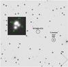 |
Fig. 1 V-band image of WFI 2033-4723 obtained by stacking the 14 best seeing and sky background images (V-band template image). The quasar and star, which we use both as a constant reference and PSF model, are labelled. The four lensed QSO components are enlarged in the darker box. The field size is 9.7 arcmin ×9.5 arcmin. The stamps used for the kernel computation are defined as 17-pixel squares (see Sect. 4). |
3. Observations
3.1. Data aquisition
The observations of the lensed quasars WFI 2033-4723 and HE 0047-1756 were obtained in the V and R bands with the 1.54 m Danish telescope at the ESO La Silla observatory, Chile, in the framework of the MiNDSTEp (Microlensing network for the detection of small terrestrial exoplanets; Dominik et al. 2010) quasar monitoring campaign. We report here on observations collected during five observing seasons from 2008 to 2012. Both quasars were observed within the following temporal intervals: from June 5 to October 4, 2008, June 19 to September 18, 2009, May 9 to August 21, 2010, June 11 to August 31, 2011, and July 16 to September 16, 2012. During these periods we observed the quasars every two days weather permitting. The V and R filters provide photometry in the Bessel system. The quasars were observed on average three times per night. WFI 2033-4723 was observed with an exposure time of 180 s in V and R, except for a small number of images, with longer exposures of 300 s and 600 s, at the start of 2008. Exposure times for HE 0047-1756 vary from 180 s in both filters during the first two seasons to 240 s in V and 210 s in R during the last three years. A few images in both bands at the start of the first season were taken with exposure times of 300 s and 600 s. The median seeing of the observations is ≈1.3 arcsec, taking both filters and all data into account. The observations were made with the Danish Faint Object Spectrograph and Camera (DFOSC) imager with a pixel scale of 0.39 arcsec. The full field of view (FOV) was 13.7 arcmin × 13.7 arcmin. We subtracted constant bias values estimated from the overscan regions to carry out bias correction and used dome flat-field frames for flat-fielding. Sections of the FOV centred on the quasars are shown in Figs. 1 and 2.
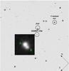 |
Fig. 2 V-band image of HE 0047-1756 obtained by stacking the 10 best seeing and sky background images (V-band template image). The quasar and stars, which we use as a constant reference and PSF model, are labelled. The double quasar is enlarged in the darker box. The field size is 8.5 arcmin ×8.8 arcmin. The stamps used for the kernel computation are defined as 17-pixel squares (see Sect. 4). |
4. The method
As was shown impressively in the case of the Huchra lens (Woźniak et al. 2000; Udalski et al. 2006), arguably the best way to carry out photometry for a quasar lens is the difference image analysis technique (DIA) proposed by Alard & Lupton (1998) and Alard (2000). The basic idea is to use a high signal-to-noise (S/N) template image, with good seeing and low sky background, which is subtracted from every other target frame in the data set. Since the lensing galaxy is not expected to vary, this approach simplifies the photometry of the quasars. As the contribution from the galaxy is removed in the subtracted images, we are spared the drawbacks of modelling the galaxy light distribution. Each pair of images needs to be astrometrically and photometrically aligned before subtraction. Relative photometry can be carried out upon subtraction. This is achieved by building a model for the quasar images with a blend of known point spread functions (PSFs) according to Hubble Space Telescope astrometry of the quasar.
In detail, the idea from Alard & Lupton (1998) is to find the best-fit, spatially non-varying convolution kernel, which degrades the template PSF into that of the target frame in addition to matching atmospheric extinction and exposure time. These authors showed that, by decomposing the kernel as a linear combination of N basis functions, the problem can be reduced to determining a finite number of kernel coefficients. The latter are found by solving a linear system of equations containing various moments of the two images in input. The analytical convolution kernel consists of a sum of several Gaussians, which are multiplied by polynomials modelling the possible asymmetry of the kernel. The Gaussian widths depend on the relative sizes of the PSF in the template and target frame. Alard (2000) extended this idea to a kernel that varies across the chip. Assuming that the amplitudes of the kernel components are polynomial functions of the pixel coordinates of order n, the number of kernel coefficients becomes  larger than in the constant kernel problem.
4.1. Image alignment
Before subtraction, all images need to be astrometrically aligned to a reference frame. After choosing a very good seeing and low sky background reference image of a given source, all the other images of the same source are registered onto the reference coordinate grid, whether or not they share the same photometric band with the reference image. This is carried out using the ISIS1 package by C. Alard (Alard & Lupton 1998; Alard 2000). The astrometric alignment routine of this package efficiently identifies reference objects (stars) in the field and carries out a two-dimensional polynomial mapping to the reference image. We choose a polynomial transformation of order 2 to remove the shifts and small rotations between the images. In the case of WFI 2033-4723, the average residuals corresponding to the astrometric transform along the x- and y-axes are of order 0.1 pixel and the mapping is computed using on average ≈275 objects. The astrometric transforms corresponding to HE 0047-1756 are characterized by average residuals of order 0.2 pixel and are obtained taking on average ≈220 objects into account. Image resampling is performed using bicubic splines. Before calling the alignment routine, bad columns are replaced with the appropriate median of surrounding pixels. All images of a given night for the whole data set are trimmed at the edges to contain the same region and median combined to improve the signal-to-noise ratio and correct for cosmic rays. After discarding images that have a high sky background or are disturbed by moonlight, clouds, bad tracking, and bad columns, we finally used 85 nights for WFI 2033-4723 and 108 nights for HE 0047-1756 over five years. V- and R-band images are not always both available for any given night.
4.2. Image subtraction
Image subtraction is carried out with the HOTPAnTS2 software by A. Becker, which is an enhanced and modified version of ISIS and the Alard (2000) method. This software is given the template image and the target frames to be processed. In creating the template images we stack the frames with the best seeing and sky background at our disposal. In the case of WFI 2033-4723 we compute the median stack of 14 images, both in V and R. A similar procedure is carried out in building the template images for HE 0047-1756, for which we were able to combine 10 frames in V and 14 frames in R. The HOTPAnTS software divides the frames horizontally and vertically into square regions, within which several stamps, centred on individual stars, are chosen. The software is also given the list of stars that act as stamps. A kernel solution is derived for each stamp. The kernel sum is used as a first metric to sigma-clip bad stamps. Briefly, the photometric scaling between two images is the sum of the convolution kernel. This can be used to discard variable stars, which are not suitable for determining the photometric alignment between the images, by sigma-clipping outlier stamps from the distribution of the kernel sums. It is useful to have multiple stars in a particular image region in case any objects are sigma-clipped. In fact at this stage another metric is used to discard bad stamps. After convolution and subtraction, the mean of the distribution of pixel residuals divided by the estimated pixel variance across each stamp provides an additional figure of merit to sigma-clip stamps out and replace them with neighbouring stars. The constraints on the convolution kernel for each stamp then allow for the fitting of the coordinate dependent amplitudes of the kernel components (modelled as polynomial functions).
For the analytical kernel we choose three Gaussians. With the aim of modelling the wings and the asymmetry of the kernel, the Gaussians are modified by multiplicative polynomials of orders 4, 3, and 2, respectively. In general we choose a narrow Gaussian that varies to order 4, a central wider Gaussian that varies at order 3, and a broad Gaussian that varies at order 2 in the kernel space coordinates. The values of the Gaussian widths σ depend on the seeing range of the templates and target frames fed to HOTPAnTS. For the target frames we compute the seeing distribution of a star in the quasar neighbourhoods in the V and R bands. We obtain the corresponding σ distribution, as shown in Fig. 3, via the relation between the FWHM and the σ of a Gaussian profile. The triplet (0.8, 1.4, 2.3) in pixel units is a good choice to build the kernel basis which, convolved with the typical template σ of 1 pixel, reproduces the typical target frame σ values. We adopt these values as our Gaussian widths. The polynomials modelling the spatial variation of the kernel amplitudes are allowed to vary at spatial order 2 in the image space coordinates.
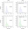 |
Fig. 3 FWHM distributions of a nearby star of WFI 2033-4723 (top) and HE 0047-1756 (bottom) in filters V (left) and R (right) in terms of the corresponding Gaussian σ. |
The number of stamps differs from case to case since it depends on the star distribution in the field. The field characterizing the frames of WFI 2033-4723 is rich with stars, while that corresponding to HE 0047-1756 is very sparse. The convolution kernel of WFI 2033-4723 is derived by taking into account on average 27 stamps in V and 26 in R; on average 8 stamps in V and 10 in R determine the convolution kernel for HE 0047-1756. The size of the stamps, 17 × 17 pixels, is chosen such that it contains the whole star flux profiles. In summary, for each image, the code chooses stamps among the stars, works out the convolution kernel and carries out the subtraction. Figures 1 and 2 show the squares defining the stamps that HOTPAnTS selects across all observing seasons in the filters V and R for the two systems.
Necessary inputs for the HOTPAnTS software are the target frame and template gain (G) and readout noise (RON). Throughout the 2008–2011 seasons the instrumental gain G was 0.76 e−/ADU and the readout noise RON was 3.21 e−. The G and RON values changed in 2012 as a result of an upgrade of the DFOSC detector between 2011 and 2012. The values that are valid for 2012 are G = 0.24 e−/ADU and RON = 5.28 e−. The gain and RON have to be adjusted appropriately before feeding them to the HOTPAnTS software. Since both the target frames and the templates are in general stacked images, we need to define an effective G and RON by using standard variance propagation.
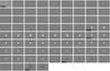 |
Fig. 4 V-band difference images of WFI 2033-4723 from 2008 to 2012. The corresponding dates are listed in Table A.1. |
Another adjustable set of parameters is the model for the sky background, which we selected to be an additive constant. The output by HOTPAnTS is the difference image with the seeing of the current target frame and the photometric scale of the template, and the corresponding noise map. Figure 4 shows the sequence of difference images for WFI 2033-4723 in filter V.
4.3. Photometry
Photometry on the difference images is carried out using the GALFIT software (version 2.0.3, Peng et al. 2002) modified to allow the fitting of several PSFs with fixed relative separations and linear fluxes. We use it to analyse the lensed quasars in the original images and in the difference images. This is performed as follows:
-
1.
A nearby star is chosen as a PSF model (the chosen stars arelabelled as PSF in Figs. 1 and 2). Weuse only one star since we noticed a remarkable variation of thePSF through the field and decided to select the closest bright,isolated, and not saturated star in the neighbourhoods. GALFITnormalizes the star so that variability is not an issue. The PSF isbuilt by extracting a 17 × 17 pixel box surrounding the star; the PSF is sky-subtracted and centred at pixel (9, 9) according to the GALFIT manual.
-
2.
Using the PSF model, the quasar positions are determined from the original stacked images and the templates with GALFIT by keeping the quasar fluxes and the position of only one of the lensed quasar images as free parameters. The sky background values at the quasar position are fixed to median values estimated from 51 × 51 pixel empty regions nearby the quasar. The positions of the remaining lensed quasar components relative to the free quasar component are kept fixed at the values shown in Table 1, which are obtained from the CASTLES3 web page (C. S. Kochanek, E. E. Falco, C. Impey, J. Lehar, B. McLeod, H.-W. Rix), as determined using Hubble Space Telescope data. Since the original stacked images and template images in general are built from a number of single exposures with different exposure times, we let GALFIT build the appropriate sigma image by providing it with the equivalent GAIN and RDNOISE of the frames, since GALFIT is only able to compute the noise image for a stack of N images with identical gain, readout noise, and exposure time. In our data we cannot significantly detect the lensing galaxies. Our positions are therefore minimally affected by the presence of the V ≈ 21 mag (WFI 2033-4723) and V ≈ 22.5 mag (HE 0047-1756) lensing galaxy.
-
3.
Keeping the nightly lensed quasar positions obtained above fixed, we determine the fluxes at the position of the quasar images in the difference images. For this, the GALFIT software is allowed to fit negative fluxes as well. The result of this procedure are difference fluxes between the epoch considered and the template image. The output noise map from HOTPAnTS is used for the difference image photometry with GALFIT. The robustness of the method just described has also been tested by computing the light curves of the four components of quasar HE 0435-1223 (Wisotzki et al. 2000, 2002), which was observed by MiNDSTEp and already published by Ricci et al. (2011), and comparing them with the results in the R band by Courbin et al. (2011). The four light curves, obtained with two different telescopes and two different methods, show an average weighted root mean square deviation of rms = 1.36σ. A similar test has been carried out by computing with this method the light curves of quasar UM673 (MacAlpine & Feldman 1982; Surdej et al. 1987, 1988; Smette et al. 1992; Eigenbrod et al. 2007), which was observed by MiNDSTEp and published by Ricci et al. (2013), and comparing the results for the two components with the results obtained in filter V and R by Koptelova et al. (2012). The average weighted root mean square deviation is rms = 1.6σ.
Hubble Space Telescope relative astrometry of WFI 2033-4723 and HE 0047-1756 images, obtained from the CASTLES webpage.
4.4. Systematics with using GALFIT
In order to test the PSF fitting with GALFIT, we created mock models of the quasar WFI 2033-4723 for three different values of the seeing in filter V. We chose to test the case of WFI 2033-4723 because it is characterized by low fluxes and highly blended components. Starting from three images of a real star in the surroundings of the quasar with FWHM 0.9, 1.31, 2.1 arcsec, using GALFIT we generated 50 artificial realizations of the quasar at each seeing value, with flux values as computed from the V template and taking those into account as mean values of the corresponding Poissonian noise. We chose the quasar centroid at each realization within one pixel with a uniform distribution. We added a sky background with mean value as computed from the V template to each artificial quasar, including Poissonian noise, and a Gaussian readout noise realization. No lensing galaxy was included in these simulations. The photometry of the artificial models was then carried out with GALFIT, choosing a PSF close to that used in building the artificial models. Figure 5 shows the distribution of the ratio Δmag /σ, which represents the difference between the GALFIT output flux and the known input flux in units of GALFIT sigmas (flux uncertainty) for quasar image A1 and for the three values of seeing. The majority of realizations lies between Δmag /σ ≈ 0−2 with minor tails at Δmag /σ ≈ 3. We find similar conclusions for the other images of the quasar. The effects, which led to the systematic discrepancy between the input and output fluxes, are determined by the differences between the PSF of the quasar and the PSF chosen to model it. The average magnitude discrepancy in the most frequent seeing regime does not exceed 0.02 mag, which is negligible for the purposes of this paper.
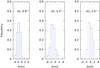 |
Fig. 5 Frequency distributions of Δm/σ; the difference between output and input magnitudes in units of GALFIT σ, for the component A1 of 50 mock models of WFI 2033-4723 under three different seeing regimes. |
5. Results
5.1. WFI 2033-4723
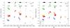 |
Fig. 6 V (left) and R (right) band light curves of WFI 2033-4723 from 2008 to 2012. Components B (filled dots), A1 (asterisks), A2 (squares), C (filled diamonds) are depicted in red, green, orange, and blue, respectively. The light curve of a star in the field, labelled as Constant star/PSF in Fig. 1, is shown in black and shifted down by 1 mag. |
Figure 6 shows the light curves for the quasar WFI 2033-4723 components B, A1, A2, C, and the constant star in Fig. 1 in filters V and R, respectively. The light curves are expressed by using instrumental magnitudes, defined as 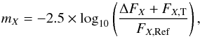 (1)where ΔFX is the flux difference of the quasar components in the subtracted image, which has the photometric scale of the template, FX,T is the corresponding flux in the template and FX,Ref that of the constant reference stars, indicated in Figs. 1 and 2, where X is V or R. Instrumental colours are defined accordingly.
The individual data points composing the light curves are also listed in Table A.1. The quoted error bars are determined by GALFIT, as explained in paragraph 4.3.3. The light curves of images B (filled dots), A1 (asterisks), A2 (squares), and C (filled diamonds) are shown in red, green, orange, and blue, respectively. The illustrated photometric data of the quasar components were shifted in accordance with the time delays measured by Vuissoz et al. (2008), namely ΔtB−C = 62.6 days and ΔtB−A = 35.5 days.
V-band and R-band yearly averages of WFI 2033-4723 instrumental magnitudes.
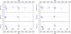 |
Fig. 7 Light curves A2-A1, B-A1, and C-A1 are shown in the V (left) and R band (right) in the upper, middle, and bottom panels, respectively. The differences are computed, after correcting for the known time delays, by interpolating in between the data points of the brightest component of each pair. The difference between C and A1 in the R band shows a significant magnitude variation of 0.16 mag between 2008 and 2011. |
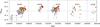 |
Fig. 8 (V−R)Instr. light curves of WFI 2033-4723 from 2008 to 2012. Components B (filled dots), A1 (asterisks), A2 (squares), and C (filled diamonds) are depicted in red, green, orange, and blue, respectively. |
Components B, A1, A2, and C become brighter in 2009 and dimmer again across the remaining seasons, spanning a magnitude range of 0.6 mag in filter V and ≈0.5 mag in filter R. We list in Table 2 the average magnitudes, computed within each season, for a more detailed picture of the brightness evolution of the four images. The quoted error bars are standard deviations computed within each season. Figure 7 is intended to reveal any differences between the variation of the four lensed components. The light curves A2-A1, B-A1, and C-A1 are shown in the V and R bands. The differences were computed upon interpolation of the brightest component at the observation dates of the weakest one in the pair, after correcting for the time delays between the pair components. The figures suggest that the variation of component C through the observing seasons differs from the others, showing a significant variation of ~0.16 mag in the R band between 2008 and 2011.
Figure 8 shows the evolution of the colour (V−R)Instr. of the four components. The four images become bluer between 2008 and 2009 by ≈0.05 mag in correspondence to the quasar brightening, and the images gradually become redder through the remaining seasons. We also compute the colour difference between the image pairs A1-B, A2-B, C-B, A1-A2, A2-C, and A1-C, after interpolating the colour of the brightest component of each pair in correspondence to the days at which the other was observed. In absence of lensing we expect the colours of the quasar components to differ only by a constant, caused by the differential intergalactic extinction along their lines of sight and by the differential reddening by the lensing galaxy. When the colour light curves of the quasar images cannot be matched by simply shifting them by a constant, the simplest explanation we can provide is microlensing affecting images in an uncorrelated fashion (Wambsganss & Paczynski 1991). We do not find systematic long-term colour difference variation across the whole observing campaign, but we cannot rule out intra-seasonal variations of order ≈0.1 mag. Intra-seasonal average values of the instrumental colour (V−R)Instr. for the four components and the colour difference between all possible pairs of components are given in Tables 3 and 4.
5.2. HE 0047-1756
In Fig. 9 we show the HE 0047-1756 light curves during the years 2008–2012 for filters V and R. The individual data points composing the light curves are also listed in Table A.2. The error bars are determined using GALFIT as explained in paragraph 3 of Sect. 4.3.
The light curves for images A and B are plotted in orange and blue, respectively, as a function of the modified Julian date (MJD). In 2008 the light curves of both lensed quasar images are characterized by a Δm ≈ 0.1 mag intrinsic variation of the quasar on timescales of ≈50 days. The data are consistent with this rise ending around MJD−2 450 000 ≈ 4680 in image A, but around MJD−2 450 000 ≈ 4690 in image B. This delay of the brightness rise in image B is analysed in detail in Sect. 5.3. In the year 2009, both quasar images became brighter. Starting from 2010 the quasar became dimmer and again brighter across the last two periods. The overall amplitude of magnitude spanned by the light curves in both filters does not exceed ≈0.3 mag. The average instrumental magnitudes of components A and B across the five periods are shown in Table 5.
Yearly averages of the instrumental colour V−RInstr. for the four lensed components of quasar WFI 2033-4723.
Yearly average differences of the instrumental colour V−RInstr. for all the possible component pairs of quasar WFI 2033-4723.
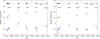 |
Fig. 9 V (left) and R (right) band light curves of HE 0047-1756 from 2008 to 2012. Components A (filled dots) and B (squares) are depicted respectively in orange and blue. The light curve of a star in the field, labelled as constant star in Fig. 2, is shown in black and shifted up by −0.7 mag. |
5.3. Time delay for HE 0047-1756
Several methods have been introduced to determine time delays in lensed systems (Kundić et al. 1997, and references therein; see also Burud et al. 2001; Gil-Merino et al. 2002; Pelt et al. 1996; and Tewes et al. 2013).
Here, we apply the PyCS software by Tewes et al. (2013) to our V and R light curves from 2008 to 2012. This software allows for time delay measurements in presence of microlensing, defined as extrinsic variability, as opposed to the intrinsic variability of the quasar. We use their free-knot spline technique and the dispersion technique. Appendix A summarizes the main input parameters for the PyCS spline and dispersion methods (see Tewes et al. 2013, for further details).
The first method uses splines to model both the intrinsic and extrinsic variability of the light curves and simultaneously adjusts the splines, time shifts, and magnitude shifts between the light curves to minimize a fitting figure of merit involving all data points. The second method goes back to the dispersion techniques by Pelt et al. (1996) and simultaneously adjusts the time shifts and low-order polynomial representations of the extrinsic variability to minimize a scalar dispersion function that quantifies the deviation between the light curves. This method does not assume any model for the intrinsic variability.
V-band and R-band yearly averages of the HE 0047-1756 instrumental magnitudes.
The results determined with the spline fitting technique and dispersion technique in the V band are 7.2 ± 3.8 days and 8.0 ± 4.2 days, respectively, with image A leading. The mean value and quoted error bars correspond to the mean and standard deviation of the resulting time delay distributions, which are obtained by drawing 1000 realizations of the observed light curves; these are shown in Figs. 10 and 11. The light curve realizations are drawn taking into account a model for the intrinsic variability, a model for extrinsic variability, and a noise model, as explained in Tewes et al. (2013). On the other hand, the application of these techniques to the R-band data in the years 2008–2012 does not converge on a unique answer. In the following we carry out a zoom-in analysis on the year 2008 in the V band only to confirm the obtained results and show that the above analysis was not biased by the existence of the observing gaps.
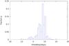 |
Fig. 10 Distribution p for time delays days based on our light curves of components AV and BV obtained by applying the PyCS dispersion method. The probability was computed from 1000 resamplings of the inferred intrinsic, extrinsic, and noise model. Mean value and standard deviation of this distribution are Δt = 8.0 ± 4.2 days. |
We found out that the best way to analyse such a short light curve portion is to follow a linear interpolation scheme, which does not introduce the difficulties of generating the model for the intrinsic and extrinsic variability, which are necessary inputs for the PyCS software to draw new realizations of the light curves, from a smaller number of data points. Our approch here, aimed at determining the time delay that minimizes the magnitude difference between the light curves, was published first by Gaynullina et al. (2005) and goes back to Kundić et al. (1997). It consists of the following steps:
-
1.
Component A of each of 10 000 bootstrapresamplings of the observed light curve is shifted by the time delayΔt to be tested, whose values lie in the range from 0 to 50 days (image A leading). Such a high number of resamplings constrains the uncertainties on the time delay measurement.
-
2.
The light curve of the brightest component A is linearly interpolated to match the dates at which the B light curve has been observed. Only gaps shorter than 20 days are interpolated.
-
3.
Each resampling is smoothed by triangular filter with a width of 3 and 6 days for the brightest component A and the weakest component B, respectively. The use of larger windows, i.e. 6 and 12 days, does not change the results.
-
4.
From the resulting light curves, comprising N epochs, we compute the weighted magnitude difference between the components Δm and the

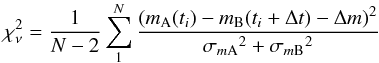 (2)is determined, where we call ti the generic time at which data has been collected. The parameters σmA and σmB are the Poissonian noise propagated through the interpolation formula for mA(ti) and the Poissonian noise corresponding to mB(ti + Δt), respectively.
 -
5.
The time delay corresponding to the minimum
is the optimal time delay at any given resampling.
The algorithm is applied to the light curve couple AVBV.
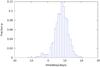 |
Fig. 11 Distribution p for time delays days based on our light curves of components AV and BV obtained by applying the PyCS spline method. The probability was computed from 1000 resamplings of the inferred intrinsic, extrinsic, and noise model. Mean value and standard deviation of this distribution are Δt = 7.2 ± 3.8 days. |
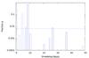 |
Fig. 12 Distribution p for time delays between 0−50 days based on our light curves of components AV and BV. The probability was computed from 10 000 bootstrap resamplings of the observed light curves. For each resampling the brightest component A was interpolated in correspondence to the dates at which B was observed. The region above the dashed line contains 95% of the statistical weight of the distribution, after discarding the peak at 0 lag. Mean value and standard deviation of this region are Δt = 7.6 ± 1.8 days. |
The probability distribution of time delays obtained using this method is plotted in Fig. 12. The probability of each 1-day bin is calculated as the ratio between the occurence of light curves with best-fitting time delay in that bin and the total number of resamplings. This procedure also produces a peak for 0 lag, which might be interpreted as a false peak, that is derived from correlated brightness fluctuations at 0 lag when dealing with optical discrete data, also reported by Vakulik et al. (2006) and Colley et al. (2003), who describes it as a “frame-to-frame correlation error in the photometry”.
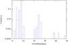 |
Fig. 13 Distribution p for time delays between 0−50 days based on our light curves of components AV, BV, and BR. The probability was computed from 10 000 bootstrap resamplings of the observed light curves. For each resampling the brightest component A was interpolated in correspondence to the dates at which B was observed. The region above the dashed line contains 95% of the statistical weight. Mean value and standard deviation of this region are Δt = 7.6 ± 2.9 days. |
We compute mean time delay and standard deviation for the region above the dashed line, which carries 95% of the statistical weight of the distribution (not taking into account the 0 lag peak), and obtain Δt = 7.6 ± 1.8 days. In order to assess whether the distribution at 0 lag corresponds to a false peak, we apply the above algorithm to the 2008 light curve couple AVBVR, where BVR is the average of the light curves of component B in both filters. The aim is to break the 0 lag correlation between the multiple photometric data recorded on a single frame. This is not strictly correct because interband time delays have been measured for several non-lensed quasars (Koptelova et al. 2010) as due to light travel time differences between two different emission regions and, in addition, the above full light curve analysis in the R band has not converged to a unique value. However, the procedure leads to a time delay distribution (shown in Fig. 13) with no peak at 0 lag, whose 95% statistical weight region is described by a mean time delay and standard deviation of Δt = 7.6 ± 2.9 days. Therefore, we conclude that the time delay analysis carried out by only taking the year 2008 into account in the V band produces a result that is consistent with the above analysis including the full light curves. In Fig. 14 we compute the difference between the light curves of components A and B in both filters. This is carried out after shifting component A ahead by 7.6 days and interpolating it at the epochs of component B. From these plots a secular evolution of the magnitude difference between the quasar components can be seen. This evolution of ≈0.2 mag across the five periods is mainly linear; we explain it as due to a long-term microlensing perturbation. Such a behaviour has already been observed for the double quasar SBS 1520+530 by Gaynullina et al. (2005).
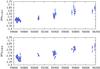 |
Fig. 14 Difference between the light curves of HE 0047-1756 components A and B after shifting component A ahead by 7.6 days. Component A is interpolated at the epochs of component B before subtraction. |
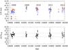 |
Fig. 15 (V−R)Instr. light curves of HE 0047-1756 from 2008 to 2012. Components A (diamonds) and B (squares) are depicted in orange and blue, respectively, in the first upper panel. In the bottom panel we show how the colour difference between the two components evolves. The difference is computed by interpolating the magnitude of the brightest component in the pair in correspondence to the dates at which the weakest one has been observed. The horizontal dashed lines define ±0.05 intervals around the average colour difference. |
An analysis of the colour index V−RInstr. light curve as a function of the MJD, shown in the upper part of Fig. 15, reveals that the two components span the highest colour variation of ≈0.07 mag between seasons 2008 and 2009, with both images turning bluer in correspondence to the 2009 brightening, as already observed by Vanden Berk et al. (2004), Pereyra et al. (2006), Ricci et al. (2011), and Ricci et al. (2013). The yearly averages of the colour are shown in Table 6.
The colour difference between the quasar images is mainly constant ≈0.04 throughout the five seasons, as shown in the bottom panel of Fig. 15. The colour difference was computed after shifting the colour light curve of component A by 7.6 days and linearly interpolating it in correspondence to the observation dates of component B. The yearly averages of the colour difference are shown in Table 7 and are consistent with a constant offset between the colour light curves.
6. Summary and discussion
We have presented V-band and R-band photometry of the gravitational lens systems WFI 2033-4723 and HE 0047-1756 from 2008 to 2012, based on data collected by MiNDSTEp with the Danish 1.54 m telescope at the ESO La Silla observatory, Chile. By applying the Alard & Lupton image subtraction method (Alard & Lupton 1998; Alard 2000) we have constructed the light curves of the quasar components.
-
1.
The lensed images of WFI 2033-4723 vary by0.6 mag in V and ≈0.5 mag in R during the campaign, becoming brighter in 2009 and gradually weaker until 2012. After computing the A2-A1, B-A1, C-A1 light curves, we note that C-A1 shows a variation of ≈0.2 mag in the R band across seasons 2008–2011. We suggest that microlensing that only affects the outer part of the accretion disk of image C could in principle explain the behaviour seen in the R band; this relies on the hypothesis that an outer and hence cooler part of the disk, with emission at longer wavelengths, is magnified by the caustic pattern.
Table 6Yearly averages of the instrumental colour V−RInstr. for the two lensed components of quasar HE 0047-1756.
Table 7Yearly average differences of the instrumental colour V−RInstr. between components A and B of quasar HE 0047-1756.
Table 8Summary of the main input parameters for the PyCS spline (spl) and dispersion (disp) methods.
-
2.
The two lensed components of quasar HE 0047-1756 reach their maximum brightness in 2009 and again in 2012 with a magnitude variation of ≈0.2–0.3 mag, depending on which components and filters are considered. For the first time we provide a measurement of the time delay between the two components. We apply the PyCS software by Tewes et al. (2013) to our whole V-band and R-band data set. The free-knot spline technique and dispersion technique provide consistent estimates of the time delay of 7.2 ± 3.8 and 8.0 ± 4.2 days in the V band. On the other hand, the two techniques do not converge to a unique result in the R band. By making use of a linear-interpolation scheme applied to the brightest component A (see Gaynullina et al. 2005), we carry out a zoom-in analysis on the year 2008 in the V band and find that the time delay value minimizing the magnitude difference between the light curves AV and BV in 2008 is Δt = 7.6 ± 1.8 days, which is consistent with the above results. The magnitude difference between the light curves of A and B in both bands increases from 2008 to 2012 by ≈0.2 mag, showing a long-term linear uncorrelation between the two components, which can be explained with a long-term microlensing perturbation.
The images of both quasars become bluer when getting brighter. This is consistent with previous studies (e.g. Vanden Berk et al. 2004). A simple possible explanation to this is obtained by considering the accretion disk models for quasars. A boost in the disk accretion rate could produce a temperature increase of the inner regions of a quasar, hence a brighter and bluer emission. The colour difference between the components of each quasar is consistent with being constant across the five periods.
Acknowledgments
We would like to thank the anonymous referee for having significantly contributed to improving the quality of this manuscript. We would like to thank Armin Rest for introducing us to the HoTPANnTS software. We also thank Ekaterina Koptelova for having provided the light curves of quasar UM673. E.G. gratefully acknowledges the support of the International Max Planck Research School for Astrophysics (IMPRS-HD) and the HGSFP. E.G. also thanks Katie Ramiré for helpful suggestions. T.A. acknowledges support from FONDECYT proyecto 11130630 and the Ministry of Economy, Development, and Tourism’s Millennium Science Initiative through grant IC120009, awarded to The Millennium Institute of Astrophysics, MAS. M.D. and M.H. are supported by NPRP grant NPRP-09-476-1-78 from the Qatar National Research Fund (a member of Qatar Foundation). M.H. acknowledges support from the Villum foundation. This publication was made possible by NPRP grant # X-019-1-006 from the Qatar National Research Fund (a member of Qatar Foundation). The research leading to these results has received funding from the European Union Seventh Framework Programme (FP7/2007-2013) under grant agreement No. 268421. T.C.H. would like to acknowledge financial support from KASI travel grant 2012-1-410-02 and Korea Research Council for Fundamental Science and Technology (KRCF). D.R. acknowledges financial support from the Spanish Ministry of Economy and Competitiveness (MINECO) under the 2011 Severo Ochoa Program MINECO SEV-2011-0187. Funding for the Stellar Astrophysics Centre is provided by The Danish National Research Foundation (grant agreement No.: DNRF106). The research is supported by the ASTERISK project (ASTERoseismic Investigations with SONG and Kepler) funded by the European Research Council (grant agreement No.: 267864). Y.D., A.E., F.F., D.R., O.W., and J. Surdej acknowledge support from the Communauté française de Belgique – Actions de recherche concertées – Académie Wallonie-Europe.
References
- Alard, C. 2000, A&AS, 144, 363 [NASA ADS] [CrossRef] [EDP Sciences] [Google Scholar]
- Alard, C., & Lupton, R. H. 1998, ApJ, 503, 325 [NASA ADS] [CrossRef] [Google Scholar]
- Burud, I., Magain, P., Sohy, S., & Hjorth, J. 2001, A&A, 380, 805 [NASA ADS] [CrossRef] [EDP Sciences] [Google Scholar]
- Chang, K., & Refsdal, S. 1979, Nature, 282, 561 [Google Scholar]
- Colley, W. N., Schild, R. E., Abajas, C., et al. 2003, ApJ, 587, 71 [NASA ADS] [CrossRef] [Google Scholar]
- Courbin, F., Chantry, V., Revaz, Y., et al. 2011, A&A, 536, A53 [NASA ADS] [CrossRef] [EDP Sciences] [Google Scholar]
- Dominik, M., Jørgensen, U. G., Rattenbury, N. J., et al. 2010, Astron. Nachr., 331, 671 [NASA ADS] [CrossRef] [Google Scholar]
- Eigenbrod, A., Courbin, F., Meylan, G., Vuissoz, C., & Magain, P. 2006, A&A, 451, 759 [NASA ADS] [CrossRef] [EDP Sciences] [Google Scholar]
- Eigenbrod, A., Courbin, F., & Meylan, G. 2007, A&A, 465, 51 [NASA ADS] [CrossRef] [EDP Sciences] [Google Scholar]
- Gaynullina, E. R., Schmidt, R. W., Akhunov, T., et al. 2005, A&A, 440, 53 [NASA ADS] [CrossRef] [EDP Sciences] [Google Scholar]
- Gil-Merino, R., Wisotzki, L., & Wambsganss, J. 2002, A&A, 381, 428 [NASA ADS] [CrossRef] [EDP Sciences] [Google Scholar]
- Gott, III, J. R. 1981, ApJ, 243, 140 [NASA ADS] [CrossRef] [Google Scholar]
- Koptelova, E., Oknyanskij, V., Artamonov, B., & Chen, W.-P. 2010, Mem. Soc. Astron. It., 81, 138 [NASA ADS] [Google Scholar]
- Koptelova, E., Chen, W. P., Chiueh, T., et al. 2012, A&A, 544, A51 [Google Scholar]
- Kundić, T., Turner, E. L., Colley, W. N., et al. 1997, ApJ, 482, 75 [NASA ADS] [CrossRef] [Google Scholar]
- MacAlpine, G. M., & Feldman, F. R. 1982, ApJ, 261, 412 [NASA ADS] [CrossRef] [Google Scholar]
- Morgan, N. D., Caldwell, J. A. R., Schechter, P. L., et al. 2004, AJ, 127, 2617 [NASA ADS] [CrossRef] [Google Scholar]
- Ofek, E. O., Maoz, D., Rix, H.-W., Kochanek, C. S., & Falco, E. E. 2006, ApJ, 641, 70 [Google Scholar]
- Pelt, J., Kayser, R., Refsdal, S., & Schramm, T. 1996, A&A, 305, 97 [NASA ADS] [Google Scholar]
- Peng, C. Y., Ho, L. C., Impey, C. D., & Rix, H.-W. 2002, AJ, 124, 266 [NASA ADS] [CrossRef] [Google Scholar]
- Pereyra, N. A., Van den Berk, D. E., Turnshek, D. A., et al. 2006, ApJ, 642, 87 [NASA ADS] [CrossRef] [Google Scholar]
- Refsdal, S. 1964, MNRAS, 128, 307 [NASA ADS] [CrossRef] [Google Scholar]
- Reimers, D., Koehler, T., & Wisotzki, L. 1996, A&AS, 115, 235 [NASA ADS] [Google Scholar]
- Ricci, D., Poels, J., Elyiv, A., et al. 2011, A&A, 528, A42 [NASA ADS] [CrossRef] [EDP Sciences] [Google Scholar]
- Ricci, D., Elyiv, A., Finet, F., et al. 2013, A&A, 551, A104 [NASA ADS] [CrossRef] [EDP Sciences] [Google Scholar]
- Smette, A., Surdej, J., Shaver, P. A., et al. 1992, ApJ, 389, 39 [NASA ADS] [CrossRef] [Google Scholar]
- Surdej, J., Magain, P., Swings, J.-P., et al. 1987, Nature, 329, 695 [Google Scholar]
- Surdej, J., Magain, P., Swings, J.-P., et al. 1988, A&A, 198, 49 [NASA ADS] [Google Scholar]
- Tewes, M., Courbin, F., & Meylan, G. 2013, A&A, 553, A120 [NASA ADS] [CrossRef] [EDP Sciences] [Google Scholar]
- Udalski, A., Szymanski, M. K., Kubiak, M., et al. 2006, Acta Astron., 56, 293 [Google Scholar]
- Vakulik, V., Schild, R., Dudinov, V., et al. 2006, A&A, 447, 905 [NASA ADS] [CrossRef] [EDP Sciences] [Google Scholar]
- Van den Berk, D. E., Wilhite, B. C., Kron, R. G., et al. 2004, ApJ, 601, 692 [NASA ADS] [CrossRef] [Google Scholar]
- Vuissoz, C., Courbin, F., Sluse, D., et al. 2008, A&A, 488, 481 [NASA ADS] [CrossRef] [EDP Sciences] [Google Scholar]
- Wambsganss, J., & Paczynski, B. 1991, AJ, 102, 864 [NASA ADS] [CrossRef] [Google Scholar]
- Wisotzki, L., Koehler, T., Groote, D., & Reimers, D. 1996, A&AS, 115, 227 [NASA ADS] [Google Scholar]
- Wisotzki, L., Christlieb, N., Bade, N., et al. 2000, A&A, 358, 77 [NASA ADS] [Google Scholar]
- Wisotzki, L., Schechter, P. L., Bradt, H. V., Heinmüller, J., & Reimers, D. 2002, A&A, 395, 17 [NASA ADS] [CrossRef] [EDP Sciences] [Google Scholar]
- Wisotzki, L., Schechter, P. L., Chen, H.-W., et al. 2004, A&A, 419, L31 [NASA ADS] [CrossRef] [EDP Sciences] [Google Scholar]
- Woźniak, P. R., Alard, C., Udalski, A., et al. 2000, ApJ, 529, 88 [NASA ADS] [CrossRef] [Google Scholar]
- Young, P., Gunn, J. E., Oke, J. B., Westphal, J. A., & Kristian, J. 1981, ApJ, 244, 736 [NASA ADS] [CrossRef] [Google Scholar]
Appendix A: Additional tables
All Tables
Hubble Space Telescope relative astrometry of WFI 2033-4723 and HE 0047-1756 images, obtained from the CASTLES webpage.
Yearly averages of the instrumental colour V−RInstr. for the four lensed components of quasar WFI 2033-4723.
Yearly average differences of the instrumental colour V−RInstr. for all the possible component pairs of quasar WFI 2033-4723.
Yearly averages of the instrumental colour V−RInstr. for the two lensed components of quasar HE 0047-1756.
Yearly average differences of the instrumental colour V−RInstr. between components A and B of quasar HE 0047-1756.
Summary of the main input parameters for the PyCS spline (spl) and dispersion (disp) methods.
All Figures
|
Fig. 1 V-band image of WFI 2033-4723 obtained by stacking the 14 best seeing and sky background images (V-band template image). The quasar and star, which we use both as a constant reference and PSF model, are labelled. The four lensed QSO components are enlarged in the darker box. The field size is 9.7 arcmin ×9.5 arcmin. The stamps used for the kernel computation are defined as 17-pixel squares (see Sect. 4). |
| In the text | |
|
Fig. 2 V-band image of HE 0047-1756 obtained by stacking the 10 best seeing and sky background images (V-band template image). The quasar and stars, which we use as a constant reference and PSF model, are labelled. The double quasar is enlarged in the darker box. The field size is 8.5 arcmin ×8.8 arcmin. The stamps used for the kernel computation are defined as 17-pixel squares (see Sect. 4). |
| In the text | |
|
Fig. 3 FWHM distributions of a nearby star of WFI 2033-4723 (top) and HE 0047-1756 (bottom) in filters V (left) and R (right) in terms of the corresponding Gaussian σ. |
| In the text | |
|
Fig. 4 V-band difference images of WFI 2033-4723 from 2008 to 2012. The corresponding dates are listed in Table A.1. |
| In the text | |
|
Fig. 5 Frequency distributions of Δm/σ; the difference between output and input magnitudes in units of GALFIT σ, for the component A1 of 50 mock models of WFI 2033-4723 under three different seeing regimes. |
| In the text | |
|
Fig. 6 V (left) and R (right) band light curves of WFI 2033-4723 from 2008 to 2012. Components B (filled dots), A1 (asterisks), A2 (squares), C (filled diamonds) are depicted in red, green, orange, and blue, respectively. The light curve of a star in the field, labelled as Constant star/PSF in Fig. 1, is shown in black and shifted down by 1 mag. |
| In the text | |
|
Fig. 7 Light curves A2-A1, B-A1, and C-A1 are shown in the V (left) and R band (right) in the upper, middle, and bottom panels, respectively. The differences are computed, after correcting for the known time delays, by interpolating in between the data points of the brightest component of each pair. The difference between C and A1 in the R band shows a significant magnitude variation of 0.16 mag between 2008 and 2011. |
| In the text | |
|
Fig. 8 (V−R)Instr. light curves of WFI 2033-4723 from 2008 to 2012. Components B (filled dots), A1 (asterisks), A2 (squares), and C (filled diamonds) are depicted in red, green, orange, and blue, respectively. |
| In the text | |
|
Fig. 9 V (left) and R (right) band light curves of HE 0047-1756 from 2008 to 2012. Components A (filled dots) and B (squares) are depicted respectively in orange and blue. The light curve of a star in the field, labelled as constant star in Fig. 2, is shown in black and shifted up by −0.7 mag. |
| In the text | |
|
Fig. 10 Distribution p for time delays days based on our light curves of components AV and BV obtained by applying the PyCS dispersion method. The probability was computed from 1000 resamplings of the inferred intrinsic, extrinsic, and noise model. Mean value and standard deviation of this distribution are Δt = 8.0 ± 4.2 days. |
| In the text | |
|
Fig. 11 Distribution p for time delays days based on our light curves of components AV and BV obtained by applying the PyCS spline method. The probability was computed from 1000 resamplings of the inferred intrinsic, extrinsic, and noise model. Mean value and standard deviation of this distribution are Δt = 7.2 ± 3.8 days. |
| In the text | |
|
Fig. 12 Distribution p for time delays between 0−50 days based on our light curves of components AV and BV. The probability was computed from 10 000 bootstrap resamplings of the observed light curves. For each resampling the brightest component A was interpolated in correspondence to the dates at which B was observed. The region above the dashed line contains 95% of the statistical weight of the distribution, after discarding the peak at 0 lag. Mean value and standard deviation of this region are Δt = 7.6 ± 1.8 days. |
| In the text | |
|
Fig. 13 Distribution p for time delays between 0−50 days based on our light curves of components AV, BV, and BR. The probability was computed from 10 000 bootstrap resamplings of the observed light curves. For each resampling the brightest component A was interpolated in correspondence to the dates at which B was observed. The region above the dashed line contains 95% of the statistical weight. Mean value and standard deviation of this region are Δt = 7.6 ± 2.9 days. |
| In the text | |
|
Fig. 14 Difference between the light curves of HE 0047-1756 components A and B after shifting component A ahead by 7.6 days. Component A is interpolated at the epochs of component B before subtraction. |
| In the text | |
|
Fig. 15 (V−R)Instr. light curves of HE 0047-1756 from 2008 to 2012. Components A (diamonds) and B (squares) are depicted in orange and blue, respectively, in the first upper panel. In the bottom panel we show how the colour difference between the two components evolves. The difference is computed by interpolating the magnitude of the brightest component in the pair in correspondence to the dates at which the weakest one has been observed. The horizontal dashed lines define ±0.05 intervals around the average colour difference. |
| In the text | |
Current usage metrics show cumulative count of Article Views (full-text article views including HTML views, PDF and ePub downloads, according to the available data) and Abstracts Views on Vision4Press platform.
Data correspond to usage on the plateform after 2015. The current usage metrics is available 48-96 hours after online publication and is updated daily on week days.
Initial download of the metrics may take a while.