| Issue |
A&A
Volume 596, December 2016
|
|
|---|---|---|
| Article Number | L2 | |
| Number of page(s) | 5 | |
| Section | Letters | |
| DOI | https://doi.org/10.1051/0004-6361/201629544 | |
| Published online | 24 November 2016 | |
Momentum-driven outflow emission from an O-type YSO
Comparing the radio jet with the molecular outflow
1 Max-Planck-Institut für Radioastronomie, Auf dem Hügel 69, 53121 Bonn, Germany
e-mail: asanna@mpifr-bonn.mpg.de
2 INAF, Osservatorio Astrofisico di Arcetri, Largo E. Fermi 5, 50125 Firenze, Italy
3 Dublin Institute for Advanced Studies, Astronomy & Astrophysics Section, 31 Fitzwilliam Place, 2 Dublin, Ireland
4 Department of Astrophysics/IMAPP, Radboud University Nijmegen, PO Box 9010, 6500 GL Nijmegen, The Netherlands
5 Instituto de Radioastronomía y Astrofísica UNAM, Apartado Postal 3-72 (Xangari), 58089 Morelia, Michoacán, Mexico
Received: 17 August 2016
Accepted: 31 October 2016
Aims. We seek to study the physical properties of the ionized jet emission in the vicinity of an O-type young stellar object (YSO) and to estimate the efficiency of the transfer of energy and momentum from small- to large-scale outflows.
Methods. We conducted Karl G. Jansky Very Large Array (VLA) observations, at both 22 and 45 GHz, of compact and faint radio continuum emission in the high-mass star-forming region G023.01−00.41 with an angular resolution between 0".3 and 0".1 and a thermal rms on the order of 10 μJy beam-1.
Results. We discovered a collimated thermal (bremsstrahlung) jet emission with a radio luminosity (Lrad) of 24 mJy kpc2 at 45 GHz in the inner 1000 AU from an O-type YSO. The radio thermal jet has an opening angle of 44° and carries a momentum rate of 8 × 10⁻³ M⊙ yr-1 km s-1. By combining the new data with previous observations of the molecular outflow and water maser shocks, we can trace the outflow emission from its driving source through the molecular clump across more than two orders of magnitude in length (500 AU–0.2 pc). We find that the momentum-transfer efficiency between the inner jet emission and the extended outflow of entrained ambient gas is near unity. This result suggests that the large-scale flow is swept up by the mechanical force of radio jet emission, which originates from within 1000 AU of the high-mass YSO.
Key words: radio continuum: stars / ISM: jets and outflows / stars: formation / stars: individual: G023.01-00.41
© ESO, 2016
1. Introduction
At the onset of the star formation process of early B- and O-type young stellar objects (YSOs), faint radio continuum emission (L8 GHz/Lbol ≲ 10-3), with a maximum extent of a few 1000 AU, is associated with radio thermal (bremsstrahlung) jets, namely, ionized gas outflowing from the inner 100s AU of the newly born star (e.g., Tanaka et al. 2016, their Fig. 18). Therefore, radio jets provide information on the outflow energetics directly produced by the star formation process (i.e., the primary outflow), as opposed to estimates of the molecular outflow energetics that are attainable on scales greater than 0.1 pc (typically through CO isotopologues). Large-scale molecular outflows, or secondary outflows, are representative of ambient gas that has been entrained by the primary outflow. To date only a handful of radio jets in the vicinity of YSOs with Lbol greater than a few 104 L⊙ have been studied in detail (e.g., Guzmán et al. 2010, and references therein).
Sensitive continuum observations at cm wavelengths, with an angular resolution on the order of  , are a major tool that can be used to resolve the spatial morphology and measure the physical properties of primary outflows (e.g., Carrasco-González et al. 2010; Hofner et al. 2011; Moscadelli et al. 2016). Here, we want to exploit the synergy between radio continuum observations and strong H2O masers, which are a preferred tracer of shocked gas at the base of (proto)stellar outflows, to quantify the primary outflow energetics within 1000 AU of an O-type YSO. Our goal is to compare primary and secondary outflow energetics and to estimate how efficiently the mass ejection in the vicinity of a high-mass YSO transfers energy and momentum into large-scale motions of the clump gas.
With this in mind, we made use of the Karl G. Jansky Very Large Array (VLA) of the NRAO1 to target the hot molecular core (HMC) of the star-forming region G023.01−00.41, where we previously detected compact (≤1″) radio continuum emission at a level of ≲1 mJy (Sanna et al. 2010). At a trigonometric distance of 4.6 kpc (Brunthaler et al. 2009), G023.01−00.41 is a luminous star-forming site with a bolometric luminosity of 4 × 10⁴ L⊙, which harbors, at its geometrical center, an accreting (late) O-type YSO (Sanna et al. 2014). In the past few years, we conducted an observational campaign with several interferometric facilities to study the environment of G023.01−00.41 from mm to cm wavelengths (Furuya et al. 2008; Sanna et al. 2010, 2014, 2015; Moscadelli et al. 2011). Of particular interest for the present study, is the detection of a collimated bipolar outflow, traced with SiO and CO gas emission at an angular resolution of 3″, which lies close to the plane of the sky at a position angle of + 58° (east of north), extends up to 0.5 pc from the HMC center, and carries a momentum rate of 6 × 10⁻³ M⊙ yr-1 km s-1 (Sanna et al. 2014).
2. Observations and calibration
Imaging information.
We observed the star-forming region G023.01−00.41 with the B-array configuration of the VLA in the K (19.0−24.3 GHz) and Q (41.6−49.8 GHz) bands. Observations were conducted under program 15A−173 during two runs on 2015 February 16 (Q band) and March 13 (K band). Scheduled on-source times were 1 h and 1.5 h, respectively. The phase center was set at RA (J2000) = 18h34m40 29 and Dec (J2000) = –9°00′38
 3. We employed the WIDAR backend and covered both continuum emission and a number of thermal and maser lines. In the following, we focus on the analysis of the continuum dataset. Continuum observations were performed using the 3-bit receivers in dual polarization mode. At K and Q bands, we employed 34 and 56 continuum spectral windows, respectively; each spectral window was 128 MHz wide. At both frequencies, bandpass and flux density scale calibration were obtained on 3C 286; complex gain calibration was obtained on J1832−1035. The QSO J1832−1035 had a bootstrap flux density of 0.938 Jy and 0.576 Jy at 22.00 GHz and 45.00 GHz, respectively.
The visibility data were calibrated with the Common Astronomy Software Applications package (CASA v 4.2.2), making use of the VLA pipeline v 1.3.1 (updated to the Perley-Butler 2013 flux density scale). After inspection and manual flagging of the dataset, we imaged the continuum emission with the task clean of CASA interactively. Figure 1 (upper) shows an overlay of the continuum emission of both frequency bands. At both K and Q bands, we achieved an image rms close to the thermal noise expected from the VLA Exposure calculator (within a factor 1.3), meaning that our maps are not dynamic-range limited. Therefore, no further self calibration was attempted. Imaging information is summarized in Table 1.
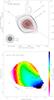 |
Fig. 1 Radio continuum emission toward G023.01−00.41. Upper: overlay of the VLA maps at K (black contours and gray scale) and Q bands (red contours). The lower five contours start at 3σ (absolute value indicated) by 1σ steps. Higher intensity levels increase by 10σ steps starting from 7σ (drawn in gray scale at K band). HPBWs are shown at the bottom left corner. The right axis gives the linear extent of the map in AU. The star indicates the HMC center, which we assume to be the YSO position (same for the lower panel; see Sect. 3). The straight line, at a position angle of + 57°, shows the best fit to the elongation of the Q-band emission (see Sect. 3). Lower: map of the radio spectral index (colors) between the K- and Q-band emission, according to the right-hand wedge. Spectral index levels are drawn on the map (black contours) together with their formal uncertainty. The red thick contour shows the 5σ of the Q-band map. Linear scales for the extension of the spectral index map are indicated. |
Radio jet properties for an isothermal conical flow with uniform ionization fraction.
3. Results
The radio continuum emission extends within 2000−3000 AU of the HMC center (star symbol in Fig. 1). The HMC center is defined by the peak position of a high-excitation (Elow of 363 K) CH3OH thermal line at the systemic velocity of the core (Sanna et al. 2014, their Table 2). In the upper panel of Fig. 1, the Q-band emission shows a spatial morphology that is stretched along the NE−SW direction with the bulk of the emission to the SW of the HMC center. On the other hand, the K-band emission shows a boxy morphology with the NE−SW diagonal line coincident with the Q-band major axis of the emission. The peak positions of the K- and Q-band maps spatially overlap at RA (J2000) = 18h34m40284 and Dec (J2000) = –9°00′3830 with an uncertainty of 30 mas in each coordinate. Despite having imaged a field of view of 0.2 pc around the radio continuum peak, we did not detect any other radio continuum source exceeding a brightness of 40 μJy beam-1 at K band (5σ).
In Fig. 1 (lower), we present a spectral index (α) map of the continuum emission between 22 and 45 GHz, which is obtained with the task clean of CASA via multifrequency synthesis cleaning and assuming a constant spectral slope (Rau & Cornwell 2011). The spectral index is computed only where the average intensity map produced by clean has S/N ≥ 10. For comparison, we also draw the 5σ contour of the Q-band emission. In this map, the levels of spectral index (and the corresponding 1σ uncertainties) are also shown in steps of 0.1. If we leave out the outer edges of the spectral index map, where the uncertainties increase to >0.1, the spectral index changes smoothly between 0.6−0.9 along the NE-SW elongation of the continuum emission. This range of values is consistent with the radio continuum emission being produced by thermal bremsstrahlung from a stellar wind (Panagia & Felli 1975; Reynolds 1986; Anglada et al. 1998). It is worth noting that the contribution of the dust emission at 7 mm should be negligible, since the 7 mm flux, which was extrapolated from our previous measurements at 3 and 1 mm (Furuya et al. 2008; Sanna et al. 2014), is less than 10% of the total Q-band flux.
In order to better discriminate the spatial morphology of the Q-band emission, we removed from the visibility dataset a point-like source model of 0.9 Jy that was set at the peak position of the Q-band map. We then cleaned the new visibility dataset with the same parameters used to produce the Q-band map of Fig. 1. The result of this procedure is shown in the right panel of Fig. 2 (hereafter, the residual map). The NE–SW extended component of the Q-band emission approaches the star position with no significant changes in shape. By fitting a two-dimensional Gaussian to the residual map, the position angle of its major axis is + 57° ± 3°. This best fit is drawn in Figs. 1 and 2. The orientation of the Q-band emission closely matches the direction (+ 58°) of the CO (2−1) outflow estimated at a scale ≳ 0.1 pc (e.g., Fig. 2, left). Combining this evidence with the spectral index analysis, we infer that the radio continuum at Q band traces a collimated thermal jet with its peak emission pinpointing a strong jet knot.
4. Discussion
 |
Fig. 2 Comparison of the outflow tracers across different scales (linear extent of each map on the right axes). Right: overlay of the K-band emission (same as in Fig. 1) with the Q-band residual map (see Sect. 3). Residual map contours start at 3σ by 1σ steps. Restoring beams and star symbol as in Fig. 1. The uncertainty of the star position is shown in the bottom left corner. For comparison, we overlay the distribution (black spots) and velocity vectors (black arrows) of the 22.2 GHz H2O maser cloudlets (Sanna et al. 2010). The gray cone indicates the boundary of the opening angle (2 ψ) of the radio jet emission (see Sect. 4). Left: comparison between the spatial distribution of the outflow entrained 12CO gas (Sanna et al. 2014) with the opening angle of the radio jet emission (gray shadow). Blue and red contours (10% steps starting from 30% of the peak emission) show the distribution of the blue- and redshifted CO gas emission with LSR velocities up to 30 km s-1 from the systemic velocity. Gray contours at the center of the bipolar outflow show the distribution of warm NH3 gas emission (Codella et al. 1997). For the NH3 map, contours start at 4σ by 1σ steps. Synthesized HPBWs are drawn at the bottom left corner. |
In Sect. 3, we have addressed the nature of the radio continuum emission and shown that the Q-band flux is dominated by thermal jet emission. In the following, we study the physical properties of this radio jet in detail. We assume the HMC center as the best guess for the YSO position. This position also coincides with the origin of the velocity fields measured with the CH3OH and H2O masers cloudlets (Sanna et al. 2010, 2015) within an uncertainty of ± 50 mas. This uncertainty does not significantly affect the following calculations.
First, we make use of the Q-band residual map (Fig. 2, right) to quantify the degree of collimation of the radio jet. At the positions of the two local peaks of the residual map, we estimate the FWHM of the jet emission ( and
and  for the stronger and fainter peak, respectively) perpendicular to the jet direction (i.e., the Q-band major axis). The jet semi-opening angle (ψ), of 22° ± 8°, is defined by the average (semi-)angle evaluated from the star position to each FWHM. In the right panel of Fig. 2, we draw the boundary of the radio jet opening angle with a gray cone. In the left panel of Fig. 2, we compare the same “radio cone” (gray shadow) with the spatial distribution of the blue- and redshifted ambient gas and show that it comprises about 70% of the CO (2−1) outflow emission.
In order to quantify the energetics of the radio jet, we derive the mass loss rate of the ionized gas following the analytic treatment by Reynolds (1986). Hereafter, we make use of the formalism introduced by these authors for a direct comparison. This approach describes the behavior of a collimated conical flow (or jet) without assuming any specific ionization mechanism. We rewrite Eq. (19) of Reynolds (1986) in a convenient form2 as follows: 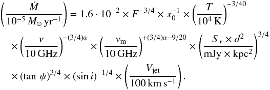 (1)The first three terms define the conditions of the ionized gas. The last six terms are the observables of the radio jet emission. The parameter F is an index for the jet optical depth, x0 is the hydrogen ionization fraction, and T is the ionized gas temperature. The radio observables are the flux (Sν), frequency (ν), and spectral index of the emission (α), the turn-over frequency of the radio jet spectrum (νm), the semi-opening angle of the radio jet (ψ), its inclination with the line of sight (i), and the expanding velocity of the ionized gas (Vjet). In Table 2, we list the values (or ranges) used to solve Eq. (1). For a 20 M⊙ star, Tanaka et al. (2016, their Fig. 3) show that the outflowing gas, in the inner 1000 AU, has a uniform ionization fraction near unity and an isothermal gas temperature of 104 K. For a pure conical flow, the Reynolds model is completely determined by these two conditions and the spectral index value of the radio jet emission. The parameter F can be directly computed with Eqs. (15) and (17) of Reynolds (1986).
In Table 2, we make use of the Q-band observations to fix ν, Sν, α, and ψ. The minimum inclination (i) of the outflow axis is set to 60° based on our SMA observations at 1 mm (Sanna et al. 2014). A lower limit to the turn-over frequency (νm) is provided by the higher frequency of the Q-band observations (50 GHz). The value of mass loss rate from Eq. (1) changes by less than 10% for any variation of i and νm in the ranges 60°−90° and 50−100 GHz, respectively.
To date, radio jet velocities between 200−1400 km s-1 have only been directly measured toward a couple of targets, as this requires long-term monitoring of the jet morphology (Marti et al. 1995; Curiel et al. 2006; Guzmán et al. 2016; Rodríguez-Kamenetzky et al. 2016). Here, we show that we can provide an estimate of the radio jet motion (Vjet) from the velocity vectors of the H2O maser cloudlets (VH2O). The 22.2 GHz H2O maser transition is a tracer of shocked ambient gas at typical densities of ~108 cm-3 (e.g., Hollenbach et al. 2013, their Fig. 15). Figure 2 (right) shows that the H2O maser cloudlets mainly lie inside the jet cone. Close to the HMC center, the H2O maser velocity field likely underlines a bow shock, which would account for the velocity vectors either parallel or perpendicular to the jet axis. The shocked layer of maser emission, further to the NE, shows velocity vectors that are well aligned with the outflow direction. Balancing the ram pressure between the ionized jet and the swept-up H2O masing gas, at a shock interface, we can derive the incoming jet velocity as a function of the H2O maser velocity along the jet direction, the pre-shocked density of the H2O gas (nH2O), and the ionized gas density (njet), 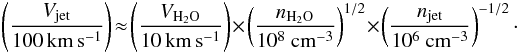 (2)Equation (2) is accurate to better than 10% provided that the density ratio between the pre-shocked and ionized gas exceeds a factor of 100. Tanaka et al. (2016) show that, in the inner 1000 AU, an ionized gas density of 106 cm-3 is most appropriate. Given a maximum H2O maser velocity of 60 km s-1 (Sanna et al. 2010), Eq. (2) implies a jet velocity of 600 km s-1 at a few 100 AU from the YSO. According to Reynolds (1986), if the flow is isothermal and uniformly ionized, a spectral index value that is higher than 0.6 corresponds to a radio jet with velocities slowly increasing with distance from the star. Taking the power-law dependence of the jet velocity with the jet radius into account, we estimate a velocity in excess of 1000 km s-1 at the southwestern tip of the Q-band map at a distance of 1700 AU from the YSO.
Finally, we draw a comparison between the mechanical properties of the radio jet and the molecular outflow (Sanna et al. 2014, Table 5). In the last columns of Table 2 we list the maximum and minimum values of mass loss (Ṁjet) and momentum rate (ṗjet) of the radio jet, for the possible combinations of radio observables, for a minimum velocity of 600 km s-1 and an outer jet velocity of 1000 km s-1. The last row of Table 2 lists the fiducial jet parameters used in the following discussion. Since we only detect the SW lobe of the jet emission at Q band, we multiply the mechanical properties of the radio jet by a factor of 2 to compare with the large-scale bipolar outflow. Asymmetric radio continuum emission is frequently observed around YSOs of different masses (e.g., Hofner et al. 2007; Johnston et al. 2013) and may be due to density inhomogeneity of the protostellar environment. Figure 2 allows one to trace the outflow emission backward, down to its driving source, over more than two orders of magnitude of distance from the HMC center (0.2 pc−500 AU). We can interpret this result as evidence for a single object dominating the clump dynamics. If the large-scale ambient gas is accelerated by the jet, the total (time-averaged) momentum released by the radio jet into the clump gas, pjet = 160 M⊙ km s-1, can be determined by multiplying the jet momentum rate by the dynamical time of the molecular outflow, tdyn = 2 × 10⁴ yr. The comparison of the momentum provided by the radio jet with that of the molecular outflow, 116 M⊙ km s-1, implies a momentum-transfer efficiency near unity. This result provides evidence that the large-scale flow is swept up by the radio thermal jet, which originates in the inner 1000 AU from the high-mass YSO.
With respect to Eq. (19) of Reynolds (1986), we assumed a pure hydrogen jet, μ/mp = 1, where μ is the mean particle mass per hydrogen atom and mp is the proton mass. Also, we replaced the parameter θ0, defined by the ratio of the FWHM of the jet (2ω0) and its distance from the star (r0), with the jet semi-opening angle, ψ (θ0 = 2 tan ψ).
Acknowledgments
Comments from an anonymous referee, which helped improve our paper, are gratefully acknowledged. Financial support by the Deutsche Forschungsgemeinschaft (DFG) Priority Program 1573 is gratefully acknowledged. The authors thank S. Dzib, P. Hofner, R. Kuiper, and A. Kölligan for fruitful discussions in preparation.
References
- Anglada, G., Villuendas, E., Estalella, R., et al. 1998, AJ, 116, 2953 [NASA ADS] [CrossRef] [Google Scholar]
- Brunthaler, A., Reid, M. J., Menten, K. M., et al. 2009, ApJ, 693, 424 [NASA ADS] [CrossRef] [Google Scholar]
- Carrasco-González, C., Rodríguez, L. F., Anglada, G., et al. 2010, Science, 330, 1209 [NASA ADS] [CrossRef] [PubMed] [Google Scholar]
- Codella, C., Testi, L., & Cesaroni, R. 1997, A&A, 325, 282 [NASA ADS] [Google Scholar]
- Curiel, S., Ho, P. T. P., Patel, N. A., et al. 2006, ApJ, 638, 878 [NASA ADS] [CrossRef] [Google Scholar]
- Furuya, R. S., Cesaroni, R., Takahashi, S., et al. 2008, ApJ, 673, 363 [NASA ADS] [CrossRef] [Google Scholar]
- Guzmán, A. E., Garay, G., & Brooks, K. J. 2010, ApJ, 725, 734 [NASA ADS] [CrossRef] [Google Scholar]
- Guzmán, A. E., Garay, G., Rodríguez, L. F., et al. 2016, ApJ, 826, 208 [NASA ADS] [CrossRef] [Google Scholar]
- Hofner, P., Cesaroni, R., Olmi, L., et al. 2007, A&A, 465, 197 [NASA ADS] [CrossRef] [EDP Sciences] [Google Scholar]
- Hofner, P., Kurtz, S., Ellingsen, S. P., et al. 2011, ApJ, 739, L17 [NASA ADS] [CrossRef] [Google Scholar]
- Hollenbach, D., Elitzur, M., & McKee, C. F. 2013, ApJ, 773, 70 [NASA ADS] [CrossRef] [Google Scholar]
- Johnston, K. G., Shepherd, D. S., Robitaille, T. P., & Wood, K. 2013, A&A, 551, A43 [NASA ADS] [CrossRef] [EDP Sciences] [Google Scholar]
- Marti, J., Rodriguez, L. F., & Reipurth, B. 1995, ApJ, 449, 184 [NASA ADS] [CrossRef] [Google Scholar]
- Moscadelli, L., Sanna, A., & Goddi, C. 2011, A&A, 536, A38 [NASA ADS] [CrossRef] [EDP Sciences] [Google Scholar]
- Moscadelli, L., Sánchez-Monge, Á., Goddi, C., et al. 2016, A&A, 585, A71 [NASA ADS] [CrossRef] [EDP Sciences] [Google Scholar]
- Panagia, N., & Felli, M. 1975, A&A, 39, 1 [NASA ADS] [Google Scholar]
- Rau, U., & Cornwell, T. J. 2011, A&A, 532, A71 [NASA ADS] [CrossRef] [EDP Sciences] [Google Scholar]
- Reynolds, S. P. 1986, ApJ, 304, 713 [NASA ADS] [CrossRef] [Google Scholar]
- Rodríguez-Kamenetzky, A., Carrasco-González, C., Araudo, A., et al. 2016, ApJ, 818, 27 [NASA ADS] [CrossRef] [Google Scholar]
- Sanna, A., Moscadelli, L., Cesaroni, R., et al. 2010, A&A, 517, A78 [NASA ADS] [CrossRef] [EDP Sciences] [Google Scholar]
- Sanna, A., Cesaroni, R., Moscadelli, L., et al. 2014, A&A, 565, A34 [NASA ADS] [CrossRef] [EDP Sciences] [Google Scholar]
- Sanna, A., Surcis, G., Moscadelli, L., et al. 2015, A&A, 583, L3 [NASA ADS] [CrossRef] [EDP Sciences] [Google Scholar]
- Tanaka, K. E. I., Tan, J. C., & Zhang, Y. 2016, ApJ, 818, 52 [NASA ADS] [CrossRef] [Google Scholar]
All Tables
Radio jet properties for an isothermal conical flow with uniform ionization fraction.
All Figures
|
Fig. 1 Radio continuum emission toward G023.01−00.41. Upper: overlay of the VLA maps at K (black contours and gray scale) and Q bands (red contours). The lower five contours start at 3σ (absolute value indicated) by 1σ steps. Higher intensity levels increase by 10σ steps starting from 7σ (drawn in gray scale at K band). HPBWs are shown at the bottom left corner. The right axis gives the linear extent of the map in AU. The star indicates the HMC center, which we assume to be the YSO position (same for the lower panel; see Sect. 3). The straight line, at a position angle of + 57°, shows the best fit to the elongation of the Q-band emission (see Sect. 3). Lower: map of the radio spectral index (colors) between the K- and Q-band emission, according to the right-hand wedge. Spectral index levels are drawn on the map (black contours) together with their formal uncertainty. The red thick contour shows the 5σ of the Q-band map. Linear scales for the extension of the spectral index map are indicated. |
| In the text | |
|
Fig. 2 Comparison of the outflow tracers across different scales (linear extent of each map on the right axes). Right: overlay of the K-band emission (same as in Fig. 1) with the Q-band residual map (see Sect. 3). Residual map contours start at 3σ by 1σ steps. Restoring beams and star symbol as in Fig. 1. The uncertainty of the star position is shown in the bottom left corner. For comparison, we overlay the distribution (black spots) and velocity vectors (black arrows) of the 22.2 GHz H2O maser cloudlets (Sanna et al. 2010). The gray cone indicates the boundary of the opening angle (2 ψ) of the radio jet emission (see Sect. 4). Left: comparison between the spatial distribution of the outflow entrained 12CO gas (Sanna et al. 2014) with the opening angle of the radio jet emission (gray shadow). Blue and red contours (10% steps starting from 30% of the peak emission) show the distribution of the blue- and redshifted CO gas emission with LSR velocities up to 30 km s-1 from the systemic velocity. Gray contours at the center of the bipolar outflow show the distribution of warm NH3 gas emission (Codella et al. 1997). For the NH3 map, contours start at 4σ by 1σ steps. Synthesized HPBWs are drawn at the bottom left corner. |
| In the text | |
Current usage metrics show cumulative count of Article Views (full-text article views including HTML views, PDF and ePub downloads, according to the available data) and Abstracts Views on Vision4Press platform.
Data correspond to usage on the plateform after 2015. The current usage metrics is available 48-96 hours after online publication and is updated daily on week days.
Initial download of the metrics may take a while.