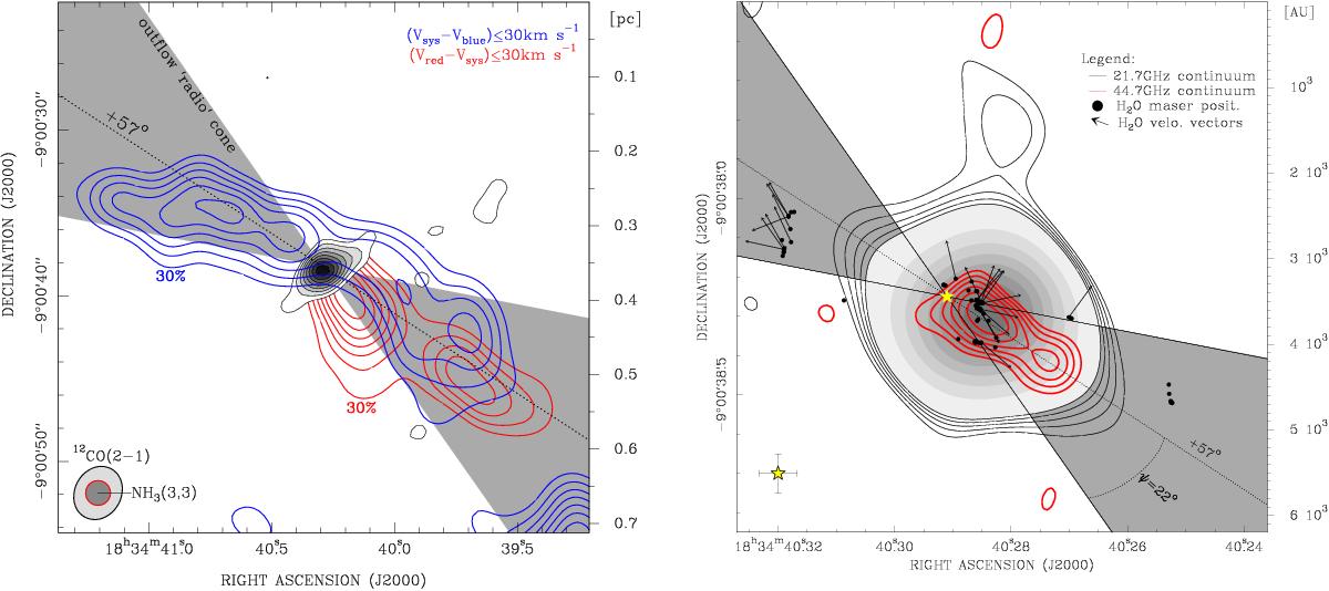
Comparison of the outflow tracers across different scales (linear extent of each map on the right axes). Right: overlay of the K-band emission (same as in Fig. 1) with the Q-band residual map (see Sect. 3). Residual map contours start at 3σ by 1σ steps. Restoring beams and star symbol as in Fig. 1. The uncertainty of the star position is shown in the bottom left corner. For comparison, we overlay the distribution (black spots) and velocity vectors (black arrows) of the 22.2 GHz H₂O maser cloudlets (Sanna et al. 2010). The gray cone indicates the boundary of the opening angle (2 ψ) of the radio jet emission (see Sect. 4). Left: comparison between the spatial distribution of the outflow entrained ¹²CO gas (Sanna et al. 2014) with the opening angle of the radio jet emission (gray shadow). Blue and red contours (10% steps starting from 30% of the peak emission) show the distribution of the blue- and redshifted CO gas emission with LSR velocities up to 30 km s^-1 from the systemic velocity. Gray contours at the center of the bipolar outflow show the distribution of warm NH₃ gas emission (Codella et al. 1997). For the NH₃ map, contours start at 4σ by 1σ steps. Synthesized HPBWs are drawn at the bottom left corner.