| Issue |
A&A
Volume 596, December 2016
|
|
|---|---|---|
| Article Number | A80 | |
| Number of page(s) | 18 | |
| Section | Extragalactic astronomy | |
| DOI | https://doi.org/10.1051/0004-6361/201629391 | |
| Published online | 05 December 2016 | |
Infrared-faint radio sources in the SERVS deep fields
Pinpointing AGNs at high redshift
1 Dipartimento di Fisica e Astronomia, Università di Bologna, viale B. Pichat 6/2, 40127 Bologna, Italy
e-mail: This email address is being protected from spambots. You need JavaScript enabled to view it.
2 Department of Physics and Astronomy, Macquarie University, Balaclava Road, North Ryde, NSW, 2109, Australia
3 INAF-IRA, via P. Gobetti 101, 40129 Bologna, Italy
4 CSIRO Astronomy & Space Science, PO Box 76, Epping, NSW 1710, Australia
5 Western Sydney University, Locked Bag 1797, Penrith South, NSW 1797, Australia
6 Australian Astronomical Observatories, PO Box 915, North Ryde, NSW 1670, Australia
7 NRAO, 520 Edgemont Road, Charlottesville, VA 22903, USA
8 Netherlands Foundation for Research in Astronomy, PO Box 2, 7990 AA Dwingeloo, The Netherlands
9 Kapteyn Astronomical Institute, University of Groningen, PO Box 800, 9700 AV Groningen, The Netherlands
Received: 25 July 2016
Accepted: 23 August 2016
Abstract
Context. Infrared-faint radio sources (IFRS) represent an unexpected class of objects which are relatively bright at radio wavelength, but unusually faint at infrared (IR) and optical wavelengths. A recent and extensive campaign on the radio-brightest IFRSs (S1.4 GHz≳ 10 mJy) has provided evidence that most of them (if not all) contain an active galactic nuclei (AGN). Still uncertain is the nature of the radio-faintest IFRSs (S1.4 GHz≲ 1 mJy).
Aims. The scope of this paper is to assess the nature of the radio-faintest IFRSs, testing their classification and improving the knowledge of their IR properties by making use of the most sensitive IR survey available so far: the Spitzer Extragalactic Representative Volume Survey (SERVS). We also explore how the criteria of IFRSs can be fine-tuned to pinpoint radio-loud AGNs at very high redshift (z > 4).
Methods. We analysed a number of IFRS samples identified in SERVS fields, including a new sample (21 sources) extracted from the Lockman Hole. 3.6 and 4.5 μm IR counterparts of the 64 sources located in the SERVS fields were searched for and, when detected, their IR properties were studied.
Results. We compared the radio/IR properties of the IR-detected IFRSs with those expected for a number of known classes of objects. We found that IR-detected IFRSs are mostly consistent with a mixture of high-redshift (z ≳ 3) radio-loud AGNs. The faintest ones (S1.4 GHz ~ 100 μJy), however, could be also associated with nearer (z ~ 2) dust-enshrouded star-burst galaxies. We also argue that, while IFRSs with radio-to-IR ratios >500 can very efficiently pinpoint radio-loud AGNs at redshift 2 < z < 4, lower radio-to-IR ratios (~100–200) are expected for higher redshift radio-loud AGNs.
Key words: galaxies: active / galaxies: high-redshift / infrared: galaxies
© ESO, 2016
1. Introduction
Infrared-faint radio sources (IFRS), first discovered by Norris et al. (2006), are a serendipitous by-product of the routine work of cross-matching catalogues taken at different wavelengths. The first IFRSs were identified in the Chandra Deep Field South (CDFS) and in the European Large Area ISO Survey South 1 (ELAIS-S1) fields, cross-matching the deep (S1.4 GHz ≥ 50–100 μJy) Australia Telescope Large Area Radio Survey (ATLAS; Norris et al. 2006; Middelberg et al. 2008), with the Spitzer Wide-Area Infrared Extragalactic Survey (SWIRE1, Lonsdale et al. 2003) at all the Infrared Array Camera (IRAC) bands (3.6, 4.5, 5.8 and 8.0 μm) and at the 24 μm band of the Multiband Imaging Photometer (MIPS).
These sources were identified as an interesting class of objects due to their lack of any IR counterpart, down to the SWIRE detection limit (Norris et al. 2006). Given the sensitivity of the SWIRE survey, it was expected that extragalactic radio sources within z~2 belonging to any known class of objects would be detected, regardless of whether the radio emission is generated by star formation or active galactic nuclei (AGN) activity, for any reasonable dust obscuration and evolutionary model. IFRSs showed a radio-to-IR flux density ratio of the order of 100 or above.
IFRS searches were later extended to the Spitzer extragalactic first look survey (xFLS; Garn & Alexander 2008) using both the 610 MHz Giant Microwave Radio Telescope (GMRT) and the 1.4 GHz Very Large Array (VLA), and to the SWIRE ELAIS-N1 field (Banfield et al. 2011) using the Dominion Radio Astrophysical Observatory (DRAO) 1.4 GHz survey (Taylor et al. 2007; Grant et al. 2010; Banfield et al. 2011), for a total of 83 IFRSs catalogued. These early samples of radio sources lacking any Spitzer counterparts cover a wide range of 1.4 GHz radio fluxes (from tenths to tens of mJy, with a preference around 1–2 mJy) and were collectively named “first generation” IFRSs (Collier et al. 2014).
A first attempt to quantify the average IR flux of these objects was performed by Norris et al. (2006), who did a stacking experiment of Spitzer data in the CDFS field, at all the IRAC bands and at the 24 μm MIPS band. Nothing was detected, implying a mean IR flux density for these objects well below the SWIRE sensitivities. Norris et al. (2006) obtained IR upper limits by stacking either the full sample of 22 sources (e.g., ≲0.5 μJy at 3.6 μm, the most sensitive IRAC band, and ≲0.03 mJy at 24 μm), or only the eight radio brightest sources to avoid any possible contamination from artefacts (e.g., ≲0.8 μJy at 3.6 μm, and ≲0.05 mJy at 24 μm). These values excluded the possibility that 1st generation IFRSs could simply belong to the dim tail of the distribution of usual classes of objects, at the same time implying that they have unusual IR properties. The result at 24 μm in particular, shows that IFRSs strongly depart from the classical mid-IR-radio correlation for star-forming galaxies (q24 = log (S24 μm/S1.4 GHz) = 0.84 ± 0.28; Appleton et al. 2004; Boyle et al. 2007; Mao et al. 2011). This suggested from the very beginning a possible AGN-driven radio emission (Norris et al. 2006; Garn & Alexander 2008; Zinn et al. 2011). The extreme ratios R3.6 = S1.4 GHz/S3.6 μm (typically ≳100) suggested to Huynh et al. (2010) and Middelberg et al. (2011) a possible link with another class of extreme objects, the high-redshift radio galaxies (HzRG). HzRG is a class of very rare sources selected from all-sky radio surveys on the basis of extreme radio-to-mid-IR ratios (R3.6≥ 200) and steep radio spectra (α ≲ −1.02), and are typically identified with radio galaxies harbouring very powerful and obscured AGNs, at redshift z > 1 (Seymour et al. 2007).
Despite these works, a comprehensive analysis of the nature of 1st generation IFRSs was challenging due to a wide variety of study-specific selection criteria. For instance, requiring the lack of an IR counterpart implies samples of IFRSs which are strongly dependent on the sensitivity of the IR survey under consideration, while fainter radio sources with no counterparts tend to have smaller R3.6. The result was a very heterogeneous class of objects.
To overcome this limitation, Zinn et al. (2011) developed a set of survey-independent criteria:
-
R3.6 > 500,
-
S3.6 μm < 30 μJy.
The first of these quantifies the ratios between radio and IR flux densities, while the second requires that these objects are at a certain cosmological distance (and is satisfied by the whole sample of 1st generation IFRSs due to the lack of any IR counterpart at the SWIRE detection limit). It is noteworthy that Zinn’s criteria tend to exclude radio-faint IFRSs, as the R3.6 criterion is more difficult to satisfy for them than the simple lack of IR counterpart. Applying these criteria, Zinn et al. (2011) extracted a list of 55 sources from four fields (xFLS, CDFS, ELAIS-S1 and COSMOlogical evolution Survey – COSMOS – fields), which represents the first sample of “second-generation” IFRSs.
Following these criteria and explicitly requiring a detected IR counterpart, Collier et al. (2014) compiled a list of 1317 IFRSs by cross-matching the Wide-field Infrared Survey Explorer (WISE; Wright et al. 2010) catalogue with the Unified Radio Catalog (URC; Kimball & Ivezić 2008). Among these sources only 19 objects have spectroscopic information available and are all identified as broad-line Type 1 quasars in the range 2 ≲ z ≲ 3.
Herzog et al. (2014) targeted with the Very Large Telescope (VLT) four 2nd generation IFRSs in the CDFS, selected to have an R-band counterpart. For three of them they successfully measured spectroscopic redshifts in the range 2 ≲ z ≲ 3, and due to the presence of broad emission lines of a few thousand km s-1, they classified them as Type 1 AGNs.
Herzog et al. (2015a) used the Very Long Baseline Array (VLBA) to target 57 IFRSs belonging to the Collier et al. list, and successfully detected compact cores in 35 of them. These targets were selected based on their proximity (distance <1 deg) to a VLBA calibrator, and on their visibility during available filler time of the VLBA array. They span a large radio flux density range (~11 → 183 mJy), which can be considered as representative of the full Collier et al. sample (~8 → 793 mJy). This confirmed that compact cores lie in the majority (if not all) of 2nd generation IFRSs, establishing them as a class of radio-loud AGN. In a more recent paper, Herzog et al. (2016) performed a comprehensive analysis of the radio spectral energy distribution (SED) of 34 out of 55 sources belonging to the original Zinn et al. (2011) list. The majority (85%) of their subsample show a steep radio SED (α < −0.8), and a significant percentage (12%) an ultra steep SED (α < −1.3, typically associated with high-z radio galaxies, see e.g. Miley & De Breuck 2008). Moreover, they found that some of these sources have a SED consistent with GHz peaked-spectrum (GPS) and compact steep-spectrum (CSS) sources, implying that at least some IFRSs are AGNs in the earliest stages of their evolution to FR I/FR II radio galaxies.
Since Collier et al. and Herzog et al. samples were limited to relatively bright radio sources (S1.4 GHz > 9 mJy), the nature of radio-faint IFRSs is still unclear. Many of the 1st generation IFRSs lie in the sub-mJy radio domain, a regime where radio sources can be associated with star-forming galaxies (SFG; see, e.g., Prandoni et al. 2001; Mignano et al. 2008; Seymour et al. 2008; Smolčić et al. 2015).
In this paper we re-analyse the IFRS samples from Norris et al. (2006), Middelberg et al. (2008), and Banfield et al. (2011), improving the earlier analyses by exploiting the deeper Spitzer extragalactic representative volume survey (SERVS3; Mauduit et al. 2012). SERVS is a deeper Spitzer follow-up of the five SWIRE fields (CDFS, ELAIS-S1, ELAIS-N1, X-ray Multi-Mirror Mission-Large Scale Structure (XMM-LSS), Lockman Hole (LH)) undertaken as part of the warm mission. As a result, SERVS reaches 5σ sensitivities of 1.9 and 2.2 μJy for the 3.6 and 4.5 μm IRAC bands, respectively (Mauduit et al. 2012). Moreover, we perform a more comprehensive analysis of the IFRS population for several ranges of R3.6, and we discuss how the R3.6 criterion can be fine-tuned to better trace this population up to high redshift (z > 4).
After a short description of the available IFRS samples in the SERVS fields (Sect. 2), we introduce a new sample extracted from the Lockman hole (LH) field (Sect. 3). Using recent 3.6 and 4.5 μm images we search for IR counterparts of all these IFRSs. The deeper SERVS data allow us to increase the number of IR detections of radio-faint IFRSs and in several cases to get information in two IR bands (Sect. 4). We present a comparison of the radio/IR properties of these sources with those of several prototypical classes of objects (Sect. 5), and we discuss the possible nature and redshift distribution of these IFRS samples (Sect. 6). Finally, in Sect. 7 we summarise our results.
Throughout this paper, we adopt a standard flat ΛCDM cosmology with H0 = 70 km s-1 Mpc-1 and ΩM = 0.30.
2. Existing first-generation IFRS samples
Main parameters of the radio, SWIRE, and SERVS surveys, together with the number of 1st generation IFRSs identified in each SWIRE and SERVS 3.6 μm field.
Radio sources without any IR counterparts down to the detection limits of the SWIRE survey were found in three SWIRE fields (CDFS, ELAIS-S1, and ELAIS-N1), and were named 1st generation IFRS by Collier et al. (2014). These samples belong to different radio surveys, characterised by different sensitivities.
CDFS and ELAIS-S1 fields were observed with the Australia Telescope Compact Array (ATCA) at 1.4 GHz in data release 1 (DR1) of the ATLAS survey (Norris et al. 2006; and Middelberg et al. 2008). ATLAS covers about 3.5 deg2 in each field, down to a typical rms sensitivity of 20–40 μJy, with spatial resolutions of 11″ × 5″ and 10″ × 7″, respectively. A new version (DR3) of the 1.4 GHz ATLAS catalogues has been recently released (Franzen et al. 2015), but we decided to keep using DR1 for consistency with previous works.
The ELAIS-N1 field was observed at 1.4 GHz down to a rms sensitivity of 55 μJy (Taylor et al. 2007; Grant et al. 2010). The observations were carried out with the Dominion Radio Astrophysical Observatory Synthesis Telescope (DRAO ST; Landecker et al. 2000), and combined with higher resolution VLA follow-up data (3.9″ × 3.9″) and with the faint images of the radio sky at twenty cm survey (FIRST; White et al. 1997, 5″ × 5″) to provide better positions (Banfield et al. 2011).
The lack of IR counterparts down to the SWIRE detection limit biased these 1st-generation samples towards radio-fainter sources, resulting in samples characterised by smaller R3.6 ratios (≳100). On the other hand, the lack of an IR counterpart is a tighter criterion than the S3.6 μm < 30 μJy one. As summarised in Table 1 (Col. 4), 22 and 29 IFRSs were identified in the CDFS and ELAIS-S1 fields, respectively (Norris et al. 2006; Middelberg et al. 2008). Another 18 IFRSs were identified in the ELAIS-N1 (Banfield et al. 2011).
When searching for IR counterparts in the deeper SERVS fields, two problems arise. First, SERVS mosaics cover smaller regions than the corresponding SWIRE ones. Therefore, the analysis is necessarily limited to sub-sets of 1st generation IFRSs, that is, those located within the 3.6 and/or 4.5 μm SERVS fields. Moreover, SERVS approaches the confusion limited flux density regime and some IFRSs lie in extremely crowded regions, increasing the likelihood of false cross-identifications. This forced us to reject three additional sources (one in the CDFS field and two in the ELAIS-N1 field: CS0283, DRAO6, and DRAO10). Of the original 69 1st generation IFRSs belonging to the three aforementioned SWIRE fields, we retain in our study only 43 sources located in the SERVS 3.6 μm mosaics (see Table 1, Col. 6). We notice that the 4.5 μm IRAC detector has a slightly shifted field of view with respect to the 3.6 μm one (Surace et al. 2005). So the total number of 1st generation IFRSs within the footprint of the 4.5 μm mosaics is slightly smaller (40 instead of 43, see Table B.1 for details).
3. New sample in the LH SERVS field
The LH field was observed at 1.4 GHz with the Westerbork Synthesis Radio Telescope (WSRT; Prandoni et al., in prep.), covering about 6 deg2 with a spatial resolution of 11′′× 9′′. This survey produced a catalogue of about 6000 radio sources down to a 5σ flux limit of 55 μJy. We searched for IFRSs in the LH field by cross-matching (searching radius of ~2 arcsec) this catalogue with the SERVS IR (3.6 μm) images and catalogues, which cover about 4.0 deg2 in the region. The search for IFRSs in this field was performed following a set of ad hoc criteria, designed to include IFRSs as faint as for 1st generation IFRSs, at the same time minimising the risk of contamination from populations of normal galaxies, typically characterised by R3.6 values ≲100 (see Norris et al. 2006).
We therefore applied a looser threshold on the radio-to-IR flux ratio than the one applied by Zinn et al. (2011), which biases IFRS samples against the faintest radio sources, by retaining as IFRSs those radio sources with R3.6 = S1.4 GHz/S3.6 μm ≥ 200 when they have a counterpart in the SERVS catalogue, and S1.4 GHz/ (2.0 μJy) ≥ 200 when they have no counterpart in the SERVS catalogue (assuming a value of 2.0 μJy as a representative SERVS 3.6 μm detection limit). Moreover we included only IR counterparts unresolved at the scale of the SERVS point spread function (PSF = 1.9′′; see Sect. 4.2 for more details), which roughly correspond to intrinsic sizes ≲32 kpc at z≳ 1. This size criterion excludes local (extended) sources that may be intrinsically faint, together with partially overlapping interacting galaxies, for which aperture photometry flux density measurements would be unreliable. This criterion is tighter than the S3.6 μm < 30 μJy constraint applied by Zinn et al. (2011), as none of our sources has S3.6 μm greater than 10 μJy (see Table B.1 for details).
As a final step we performed a visual inspection of the 3.6 μm images for all the candidate IFRSs, and we removed the sources in crowded regions (i.e., for which the cross-matching is doubtful), those of uncertain radio position (e.g., due to a complex radio shape), and those coinciding with catalogued radio lobes. In the end, in the LH field we retained 21 sources at 3.6 μm, 19 of which fall inside the 4.5 μm mosaic footprint.
In summary, our analysis was carried out on a total of 64 sources, 59 of which fall inside the 4.5 μm mosaic footprint (see Table B.1 for details).
4. Flux density measurement at 3.6 and 4.5 μm
Flux densities at 3.6 and 4.5 μm for all the sources in the SERVS deep fields were measured on the SERVS mosaics using a standardised procedure. Our flux density measurement includes three steps: (1) correction for systematic offsets between radio and IR catalogues; (2) extraction of the IR image cutouts centred on the corrected radio positions; (3) flux density measurement through the aperture photometry technique.
4.1. Correction for radio-IR positional offsets and extraction of image cutouts
Positional offsets were established by cross-matching the ATLAS and SERVS catalogues for the CDFS and ELAIS-S1 fields, and the WSRT and SERVS catalogues for the LH field. For the ELAIS-N1 field we used the FIRST survey (see Sect. 2), as the original DRAO observations have too poor spatial resolution (42″ × 69″).
For each field and SERVS frequency we cross-matched the radio and SERVS source catalogues, and derived the distribution of the separation between closest matches. We defined the systematic offsets as the position of the peak of the Gaussians fitting the radio-IR separation distributions. We show the result in Table 2. Some offsets are larger than the SERVS positional accuracies (0.1–0.2′′), but all are well below the SERVS PSF (~2″ × 2″; Mauduit et al. 2012).
We then corrected the radio positions for the corresponding offsets, and extracted 3.6 and 4.5 μm cutouts from the SERVS mosaics, each centred at the corrected IFRS radio position. The cutouts are 99 × 99 pixels (i.e., 30 × 30 SERVS PSFs) wide.
Radio-IR positional offsets for each field, both for 3.6 and 4.5 μm catalogues.
4.2. Aperture photometry at 3.6 and 4.5 μm
For each cutout, we used the DAOPHOT IRAF4 task to measure the flux density through the aperture photometry technique, either at the centre of the cutouts (when no source was visually identified) or at the nearest IR source position (when a likely IR counterpart was present). We set the aperture radius to 1.9′′, which roughly corresponds to the PSF of SERVS point sources (Mauduit et al. 2012). Finally, we multiplied the measured flux densities for the IRAC aperture corrections corresponding to that radius (1.359 for the 3.6 μm band and 1.397 for the 4.5 μm band; Surace et al. 2005).
The uncertainties in the measured aperture flux densities were again estimated using the DAOPHOT task. We built a grid of 15 × 15 apertures for each cutout and we computed the flux density from each aperture. For each cutout, the distribution of such flux densities was fitted by a Gaussian. Then, we iteratively rejected the >3σ outliers (likely contaminated by the presence of a source) until the process converged. The standard deviation of the final Gaussian distribution is a measure of the local root mean square (rms) of the cutout and provides an estimate of the error on the flux density measurement. In case of non-detections, an (3× local rms) upper limit is provided.
This procedure allowed us to look for detections below the 5σ threshold of the SERVS catalogues. We notice that some of the brightest sources are listed in the SERVS catalogues and the flux densities we derived are consistent with those provided in the catalogues. On the other hand, our flux density errors are larger and have to be considered as more conservative. For consistency we adopted our flux density (and error) estimates for all sources, disregarding any presence in the SERVS catalogues.
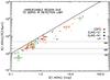 |
Fig. 1 1.4 GHz-to-3.6 μm flux density ratios versus 1.4 GHz radio flux density. The diagonal solid line marks the lowest R3.6 values we can trace due to the combined radio and SERVS detection limits (derived assuming S1.4 GHz > 100 μJy and S3.6 μm > 1 μJy, i.e., the smallest lower limit we measure in our sample). The dotted lines indicate flux density ratios R3.6 = 100, 200, and 500. Flux ratios for reliably IR-detected IFRSs are reported as crosses (position with errors bars), while flux ratios of IR undetected/unreliable sources are indicated by triangles (lower limits). To each field corresponds a different colour, as explained in the legend. |
4.3. Reliability of SERVS counterparts
We used the likelihood ratio technique (e.g. Ciliegi et al. 2003) to compute the reliability of the SERVS counterparts, that is, the probability of finding neither a chance identification nor a peak noise closer to the radio source than the IR candidate. The reliability was computed for both 3.6 and 4.5 μm counterparts, and typically it ranges from 70% to 99% (Col. 9, Table B.1). To avoid contamination by false-positive identifications, in any following analysis we only retain SERVS counterparts with a reliability of >90%, while we consider as undetected all IFRSs with no (or unreliable) SERVS counterparts.
In total we found 21 reliable counterparts at 3.6 and 20 at 4.5 μm, for a total of 25 distinct IFRSs out of the original 64 sources we analysed (see Sect. 3). When identified at both bands, the reliability constraint (>90%) is satisfied at both 3.6 and 4.5 μm. The SERVS cutouts of all IFRS with reliable SERVS counterparts are shown in Appendix A. For the LH IFRSs we also show the radio contours.
We also estimated the false detection rate, by searching for serendipitous detections with a reliability of >90%. This was done by shifting the positions of the radio sources by an amount between 50′′ and 500′′ in 100 steps spiralling outward, and measuring the aperture photometry at each of such positions. False detection rates range from 5 to 8% (depending on the field and on the band), so we expect that around two counterparts out of the 41 (21 at 3.6 and 20 at 4.5 μm) retained as reliable IFRS are false.
4.4. Information at other wavelengths
The only previous attempt to search for IFRS IR counterparts using SERVS data was performed by Norris et al. (2011) who used a pre-release of the 3.6 μm images. They detected three out of 39 1st generation IFRSs in the CDFS and ELAIS-S1 SERVS fields (CS0114, with S3.6 μm = 2.20 ± 0.54 μJy; CS0173, with S3.6 μm = 2.14 ± 0.65 μJy; and CS0255, with S3.6 μm = 1.91 ± 0.53 μJy), but concluded that all detections were consistent with being chance associations caused by confusion. These three sources are detected also by us, with similar flux densities. Due to our slightly deeper SERVS mosaics and improved cross-matching algorithm, we are confident that most of our detections are not chance associations.
In Table B.1 we list the 3.6 and 4.5 μm aperture flux densities and errors (or the 3σ upper limits in case of no detection or unreliable SERVS identification) measured for all the sources in the SERVS fields (Cols. 11 and 12). Also listed are the derived radio-to-IR flux ratios or upper limits (Cols. 13 and 14), and the 4.5-to-3.6 μm flux ratios or upper (or lower) limits in case of detection at only one band (Col. 15). The new SERVS mosaics allowed us to get reliable IR counterparts for 21 IFRSs at 3.6 μm, for 20 at 4.5 μm, and for 16 in both bands. All detected sources have IR fluxes of a few μJy, typically with S/N ~ 3–10. The three sources associated with crowded regions and discarded (see Sect. 2) are marked with “–” in all IR-related columns. The IFRSs which are located outside the 4.5 μm footprint are marked “out” in the 4.5 μm flux density column.
For six sources we have found an optical counterpart. These counterparts have been identified by imposing a maximum search radius of 2′′ around the radio source position, and belong to a number of independent surveys as listed at the end of Table B.1. With only one exception (LH3817, with KAB = 20.75), the optical magnitudes of these objects are very faint (AB magnitudes ≳24, see Table B.1, Col. 17), suggesting high redshifts. None of the reliable optical counterparts has a measured redshift.
4.5. IFRS radio-to-IR ratio distribution
Figure 1 shows the R3.6 ratios (or corresponding lower limits) versus 1.4 GHz flux density for all the sources in the SERVS fields. The solid diagonal line represents the R3.6 detection limit. It is noteworthy that sources not detected in SERVS or with unreliable identifications (triangles) span the entire range in radio flux probed by our samples.
In Table 3 we list the number of IFRSs found in each field (CDFS, ELAIS-S1, ELAIS-N1, LH) for different ranges of R3.6 (<100, 100–200, 200–500, and >500). In the case of IR undetected sources (or unreliable identifications), we assign the source to the R3.6 range constrained by the estimated lower limit value. Sources with R3.6< 200 cannot be found in the LH field, as we imposed a minimum threshold of 200 for our IFRS search (see Sect. 3). Considering that several sources have R3.6 lower limits, at least 60% of the 55 sources with R3.6 > 200 satisfy the Zinn et al.R3.6> 500 criterion, and most of them have S1.4 GHz > 1 mJy. This is consistent with the fact that this criterion tends to exclude faint radio sources, as discussed in Sect. 1. Only three sources in the ELAIS-S1 field show very low radio-to-IR ratios (R3.6 < 100) based on our new SERVS analysis, and can be explained in terms of normal galaxy populations. All these sources have S1.4 GHz < 0.2 mJy. The rest of the sub-mJy sources (S1.4 GHz ~ 0.3–1 mJy) typically have R3.6~100–500. They do not satisfy the stringent Zinn et al.R3.6 > 500 criterion, but nonetheless display extreme IR properties.
Statistics of IFRSs in the SERVS fields as a function of radio-to-IR flux ratio (R3.6).
4.6. Average IR flux densities of undetected sources
We performed a median stacking analysis of the sources with no or unreliable counterparts at the SERVS flux limits, focusing our analysis on IFRSs with R3.6 > 500 (22 at 3.6 μm and 20 at 4.5 μm), to explore down to a fainter regime the IR properties of this extreme population. After stacking the SERVS image cutouts, 3.6 and 4.5 μm median flux densities were measured through aperture photometry, and flux errors were estimated as explained in Sect. 4, except that median stacking removes the need to reject >3σ outliers (see Sect. 4.2).
No secure detection was obtained in the stacked image. At 3.6 μm we find a median flux density upper limit of  < 0.46 μJy, and for the first time we provide a median upper limit at SERVS 4.5 μm,
  < 0.60 μJy (both 3σ values). The total lack of detection in the stacked images highlights how the counterparts distribution is probably dominated by sources well below the SERVS detection limit, with actual R3.6 values significantly larger than 500.
Norris et al. (2011) also attempted a stacking experiment based on preliminary SERVS images of ATLAS fields, obtaining a median flux density of < 0.42 μJy. The two 3.6 μm upper limits are remarkably similar despite the fact that some of the sources stacked by Norris et al. (2011) are detected by us at the level of few μJy. Our upper limit is slightly larger due to the fact that a smaller number of sources were stacked. The most notable differences between the sample of sources we stacked and the one stacked by Norris et al. (2011), is that we expanded the sample to two new fields but removed from the stacking all the sources with R3.6 < 500. Most of these sources are very faint radio sources (S1.4 GHz≲ 0.5 mJy), and some have not been detected in ATLAS DR3 (Franzen et al. 2015). These sources (CS0275, CS0696, CS0706, CS0714, ES0135, ES1118, and ES1193) may be the result of unusual noise peaks or imaging artefacts.
Main modelling parameters.
5. Models of comparison
Our sample spans a much larger range in both R3.6 ratio and radio flux density than the “bright” Collier et al. (2014) and Herzog et al. (2014) samples. Lower flux densities and lower R3.6 values can be explained as the result of the same IR properties but lower intrinsic radio luminosities, associated with a population of less radio-loud quasi-stellar objects (QSO). Alternatively it can be the result of a more diverse population and/or redshift distribution. Indeed several of our sources lie in the radio sub-mJy regime, where radio sources consist of both AGNs and SFGs (see e.g., Prandoni et al. 2001; Mignano et al. 2008; Seymour et al. 2008; Smolčić et al. 2015).
To disentangle these different scenarios, we need to compare the radio and IR properties of our IFRSs with those of known classes of objects, including the effects of evolution and dust extinction. To build our reference models we used the spectral energy distribution (SED) templates from the SWIRE template library (Polletta et al. 2007). In particular we used the templates of Arp 220 (as representative of star-burst galaxies), of Mrk 231 (as representative of composite Seyfert 1 and starburst objects), of IRAS 19254-7245 (hereafter I19254, as representative of a composite Seyfert 2 and starburst objects), of a 5 Gyr old Elliptical (for the hosts of elliptical radio-loud galaxies, RLG), Seyfert 1 and 2 average templates for Type 1 and 2 AGNs, respectively, and QSO1 and QSO2 templates for average Type 1 and Type 2 QSOs.
We included the effect of K-correction and intrinsic evolution. For both IR and radio bands, and for all classes of objects, we assumed pure luminosity evolution (PLE), and in particular we used models accounting for a luminosity damping at high redshift (z≳ 2). We K-corrected 1.4 GHz flux densities by assuming a power law spectrum (S ∝ να), assuming indicative reference values for the spectral index. We assumed α = −1.0 for typically steep-spectrum sources (Arp 220, RLGs, I19254, Type 2 AGNs, and Type 2 QSOs), and α = 0 for typically flat-spectrum sources (Mrk 231, Type 1 AGN, and Type 1 QSOs). The 3.6 and 4.5 μm flux densities were K-corrected using the Hyperz software (Bolzonella et al. 2000).
The intrinsic IR luminosity evolution was modelled following Stefanon & Marchesini (2013), who derived PLE models for normal galaxy populations in both rest-frame H- and J-bands, and following Assef et al. (2011), who derived PLE models for AGNs in the rest-frame J-band. In particular we used the former models for Arp 220 and RLGs, and the latter for Mrk 231, I19254, AGNs, and QSOs. The intrinsic IR luminosity evolution for each class of objects was modelled following the evolution of the characteristic luminosity (L∗), that is, the luminosity which marks the change from power law to exponential regime in the Schechter luminosity function.
Other models are available in the literature for a number of rest-frame IR bands (see e.g., Pozzetti et al. 2003; Babbedge et al. 2006; Saracco et al. 2006; Dai et al. 2009). For our toy models, however, subtle differences are not relevant, as we are interested only in obtaining overall reference evolutionary tracks. Our final choice was mainly dictated by: a) the wider redshift range probed by the selected models (z < 3.5 for Stefanon & Marchesini 2013; z < 5 for Assef et al. 2011), which reduces the uncertainties introduced when such models are extrapolated to higher redshifts; b) the fact that analytical forms were used to describe the evolution that take into account in a single law both positive luminosity evolution at low redshifts and luminosity damping at high redshifts (z≳ 2).
For Type 1 and 2 AGNs, Type 1 and 2 QSOs, and for RLGs we assumed as reference IR luminosity (L0 ≡ L∗(z = 0)), the characteristic luminosity expected for these classes of objects at redshift z = 0, following Assef et al. (2011) and Stefanon & Marchesini (2013), respectively. For Mrk 231, Arp 220, and I10254 we assumed their own luminosity. In particular we fixed the 3.6 μm luminosity and scaled it to 4.5 μm following the templates.
We modelled the radio luminosity evolution of high power (L≳ 1025 W Hz-1) AGNs and composite AGN plus starburst galaxies following Dunlop & Peacock (1990). In particular we applied the PLE model derived for steep-spectrum radio sources to high-power RLGs, Type 2 AGNs, Type 2 QSOs, and I19254, and the flat-spectrum model to Type 1 AGNs, Type 1 QSOs, and Mrk 231. Two reference radio powers (L0 ≡ L(z = 0)) were assumed for RLGs, as well as for Type 1 and 2 QSOs. For RLGs, the low-power luminosity was assumed 1024 W Hz-1, while the high-power luminosity is 1026 W Hz-1. For Type 1 and 2 QSOs the low-power luminosity is higher than for RLGs (1025 W Hz-1), while the high-power luminosity is the same (1026 W Hz-1). For Mrk 231 and IC19254 we assumed 1024 W Hz-1, which is approximately equal to their actual radio powers.
The radio luminosity of low-power (L≲ 1024 W Hz-1) radio-loud (RL) AGNs associated to elliptical galaxies is known to evolve less strongly, and is typically modelled with a law of the form L(z) = L0(1 + z)β up to a given maximum redshift zmax, and L(z) = L(zmax) at higher redshifts. Following Hopkins (2004) we assumed β = 2, while zmax was set to two (this is likely to be a generous assumption as there are growing indications that the number density of low-power RL AGN peaks at redshift z≲ 1; see e.g., Padovani et al. 2015).
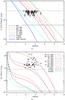 |
Fig. 2 Expected flux densities versus redshift for our models: Type 2 and Type 1 AGNs (dotted black and long-dashed grey tracks, respectively); Type 2 and Type 1 QSOs (triple dot-dashed orange and dot-dashed magenta tracks, respectively); radio galaxies (long-dashed green for high-power and dark green for low-power tracks); Arp 220, without and with reddening (dotted cyan and solid blue tracks, respectively), Mrk 231 (dashed red track), and I19254 (long-dashed brown track). Superimposed are the Collier et al. (2014) and Herzog et al. (2014) IFRSs with measured redshift (empty diamonds and empty squares, respectively). Panel a) – Top: IR fluxes at 3.4 (WISE)/3.6 (SWIRE) μm versus redshift; the dashed horizontal line represents the 30 μJy flux density threshold used by Collier et al. (2014) and Herzog et al. (2014) to select their IFRS samples, while the solid horizontal line represents the largest flux density measured in our sample (LH2633, S3.6 μm~5.43 μJy). Panel b) – Bottom: 1.4 GHz radio flux density versus redshift; high-power Type 2 QSO and RLG trends are superimposed due to the identical modelling we applied, as well as for Type 1 AGN and low-power type 1 QSO, and for Type 2 AGN and low-power Type 2 QSO (see Table 4). The dashed horizontal line indicates the lowest 1.4 GHz flux density measured in Collier et al. (2014) and Herzog et al. (2014) samples (7.98 mJy, see Sect. 1), while the solid horizontal line indicates the lowest 1.4 GHz flux density measured in our sample (ES0463, S1.4 GHz~0.14 mJy, see Table B.1). |
The same evolutionary form is also used to model the radio luminosity of starburst galaxies (Arp 220-like objects). Typically β has values between 2.5 and 3.33 (see e.g., Saunders et al. 1990; Machalski & Godlowski 2000; Sadler et al. 2002; Seymour et al. 2004; Mao et al. 2012) and zmax is typically assumed to be in the range of 1.5–2. We assumed β = 3.3 and zmax = 2 (Hopkins et al. 1998; Hopkins 2004). This is a rough approximation, as it is known that the radio luminosity at high redshift starts to decrease, but this approximation covers well enough the redshift range within which such a source would be still detectable by our radio surveys. The L0 parameter was set equal to the actual 1.4 GHz radio luminosity of Arp 220 (2 × 10²³ W Hz-1). Table 4 summarises the reference powers and the evolutionary models applied to our templates, and the redshift range within which these models have been derived.
In panels a and b of Fig. 2, we show the IR and 1.4 GHz evolutionary tracks expected for our models, while Fig. 3 shows the expected R3.6 versus redshift relation. In this case, each track is truncated at the redshift at which the radio flux density drops below the typical detection limit of the radio surveys under consideration (S1.4 GHz~0.1 mJy, see Table 1). For AGN and QSO templates, the expected radio-to-IR R3.6 ratio tends to increase with redshift up to z~2–3, due to the positive radio evolution being stronger than positive IR evolution. Then the ratio starts to decrease due to the steeper decline in the radio evolution. QSOs, AGNs, and high-power RLGs are the only classes of objects able to reach R3.6≳ 100, further supporting previous evidence that IFRSs host an AGN. Arp 220 (dotted cyan line) keeps increasing up to the highest redshifts at which this source would be still detectable in our surveys, but never reaches the lowest R3.6≳ 50 values measured in our faint IFRS sample. The same is true for Mrk 231, low-power RLGs, and I19254.
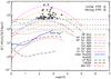 |
Fig. 3 R3.6 ratio evolutionary tracks; in this plot each track is truncated at the redshift at which the radio flux density drops below the detection limit S1.4 GHz ~ 100 μJy. The horizontal dashed lines indicate R3.6 ratios of 100, 200, and 500. The errors associated to the measured R3.6 ratios of the Collier et al. (2014) and Herzog et al. (2014) samples are of the same magnitude of the symbols reported in the plot, and not shown. At the end of the Arp 220 reddened track we indicate the star formation rate expected for this source if it were at redshift ~3, under the hypothesis that star-forming activity entirely accounts for the radio emission in this object. |
As pointed out by Norris et al. (2011), radio-to-IR ratios can be increased by introducing some level of dust extinction. We explored this effect for Arp 220 by modelling the extinction as a power law of the form Aλ∝λα (Whittet 1988), with α = −2.20 (see, e.g., Stead & Hoare 2009; Schödel et al. 2010; Fritz et al. 2011). In Fig. 2 (panel a) and Fig. 3, the reddened track of Arp 220 is indicated by the solid blue line. At the end of this track, the star-formation rate expected for Arp 220 at that redshift (3600 M⊙ yr-1) is reported, under the hypothesis that star-formation activity entirely accounts for the radio emission in this object. This value has been obtained following Condon (1992). Even in this case, starburst Arp 220-like galaxies hardly reach R3.6~100, but can account for the few objects in our IFRS sample with R3.6≲ 100.
We notice that the evolutionary tracks shown in panels a and b of Fig. 2 are sensitive to the assumed reference luminosity and therefore should be used with caution. Figure 3, on the other hand, is more robust as it only depends on the ratio between the radio and IR flux densities. As a sanity check, in both panels of Fig. 2 and in Fig. 3, we also show the flux densities and/or the R3.6 values of all Collier et al. (2014) and Herzog et al. (2014) bright IFRSs for which a redshift was measured (empty diamonds and empty squares, respectively). All such IFRSs are classified as broad-line Type 1 QSOs. The only tracks that can reproduce their IR and radio properties (see panels a and b of Fig. 2), as well as the R3.6≳ 500 selection criterion imposed for these IFRSs (see Fig. 3), are the ones of QSOs and high-power (HP) RLGs. In general, the spectral indices of the Collier et al. (2014) IFRSs with measured redshift are flat (see Sect. 1), pointing towards a core-dominated Type 1 QSO population, in excellent agreement with the spectroscopic classification of the IFRSs. The two IFRSs from Herzog et al. (2014) with redshifts, for which a spectral index was measured, show steep spectra (−0.84 for CS0212, −0.75 for CS0265), possibly indicating that these sources are RL QSO, dominated by optically thin synchrotron emissions from the radio jets.
As shown by the horizontal solid lines in Fig. 2, our sample probes much lower radio and IR flux density ranges than the Collier et al. (2014) and Herzog et al. (2014) samples, possibly associated to different source types and/or redshift distribution. This will be investigated in Sect. 6.
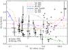 |
Fig. 4 S4.5 μm/S3.6 μm ratios versus 1.4 GHz flux density for IFRS sources. Sources detected only at one IR band (either 3.6 or 4.5 μm), are indicated by the corresponding upper or lower limits. The dashed horizontal lines refer to S4.5 μm/S3.6 μm ratios equal to 1.0, 1.5, and 2.0 respectively. The superimposed tracks refer to HP Type 2 and 1 QSOs (triple dot-dashed orange and dot-dashed magenta respectively), HP RLGs (long-dashed green), Type 1 and 2 AGNs (dashed and dotted grey, respectively), and reddened Arp 220 (solid blue). The redshift increases along the tracks toward the left-hand side of the plot; unitary increments in redshift are marked by dots, starting from the value reported near the first dot on each track. LP QSOs would show a similar track to HP QSOs, but slightly shifted to the left, and are not shown. All the tracks have been drawn in the redshift range within which R3.6 > 50, which is close to the smaller value we measured for our IFRSs (see Table B.1). Empty diamonds and empty squares represent the positions of the IFRSs with redshift from Collier et al. (2014) and Herzog et al. (2014), respectively. In the top-right corner of the plot are shown the median errors for these two samples. Upward empty and filled triangles indicate IFRSs from our sample with R3.6> 500 and between 200 and 500, respectively. The two radio-faintest sources are ES0593 and ES0436, both with R3.6 values below 100. None of the reliably identified IFRSs shown in this plot has R3.6 between 100 and 200. |
6. Radio/IR properties of SERVS deep field samples
We used the evolutionary tracks described in Sect. 5 to assess the nature of our ≳10× fainter IFRSs, spanning a larger range of R3.6 values (i.e. R3.6 ≳ 50–100). In the absence of redshift information, we explored the radio and IR properties of our sample in the parameter space defined by the S4.5 μm/S3.6 μm flux density ratio against the 1.4 GHz radio flux. This choice has the advantage of being independent of the assumed reference IR luminosity, while different radio luminosities just produce an horizontal shift of the evolutionary tracks.
The results are shown in Fig. 4, in which we plot only those IFRSs detected at either 3.6 or 4.5 μm, or both. Our IFRSs typically have S4.5 μm/S3.6 μm flux ratios in the range of 1–2. Due to the very large error bars ( = 0.35 for our sample), it is difficult to say if any source has the most extreme values S4.5 μm/S3.6 μm ≥ 2. Different symbols correspond to different R3.6 ranges: R3.6 > 500 (empty triangles), 200 < R3.6 < 500 (filled triangles), R3.6 < 100 (error bars only). None of the reliably identified IFRS shown in Fig. 4 has 100 < R3.6 < 200.
Superimposed are the evolutionary tracks of the classes discussed in Sect. 5 (following the same colour and line style convention as in Fig. 2), that can produce R3.6 > 50 (namely Type 1 and 2 QSOs, HP RLGs, Type 1 and 2 AGNs, and reddened Arp 220). The redshift increases along the tracks toward the left-hand side of the plot, and each unitary increment of redshift is marked with a dot of the same colour of the track. The first of these dots reports also the first unit redshift of that track. Overall, the S4.5 μm/S3.6 μm flux ratios spanned by our models cover the entire range spanned by our IFRS sample, indicating that our models can account for the whole faint IFRS population.
In Fig. 4 we also show the brighter IFRSs from Collier et al. (2014) and Herzog et al. (2014). The median errors on their IR ratios are shown in the upper right corner of the figure ( = 0.46 and = 0.06 for Collier et al. 2014; and Herzog et al. 2014, respectively). Considering the large error bars, all these IFRSs are again consistent with a QSO classification. Our fainter IFRS sources are mostly consistent with being higher redshift counterparts of Collier et al. (2014) and Herzog et al. (2014) IFRSs. Sources with R3.6 > 500 would be QSOs at redshifts z~3–4, while IFRSs with less extreme R3.6 (100 < R3.6 < 500) would lie at a higher redshift (z > 4). This is consistent with the expected R3.6 vs. redshift relation of QSOs reported in Fig. 3. Only the IFRSs with lowest S4.5 μm/S3.6 μm flux ratios (~1) are better described by the HP RLG track, and their R3.6 values are again consistent with the expected R3.6 vs. redshift relation.
We notice that Type 1 and 2 AGN tracks can also account for R3.6 < 500 IFRSs. Therefore, the fainter IFRS population could in principle either be associated to very high redshift QSOs or to Type 1 and 2 AGNs at less extreme redshift (2 < z < 4), or a mixture of both.
Our faint IFRS sources have average radio spectral properties in line with Herzog et al. (2014) IFRSs. Franzen et al. (2015) reported the spectral indices computed between 1.40 and 1.71 GHz, values that are consistent with the ones computed between 1.4 GHz (from low-resolution data) and 2.3 GHz by Zinn et al. (2012), and with the ones reported by Middelberg et al. (2008). 21 of our sources in the CDFS and ELAIS-S1 have measured spectral indices (see Table B.1, Col. 16). 13 of them have R3.6 > 500, and their median spectral index is very steep ( = −1.05), while eight of them have 200 <R3.6< 500, and their median spectral index is ( = −0.72). A steep-spectrum population is more consistent with a Type 2 QSO and Type 2 AGN or RLG classification.
As a final remark, we notice that the faintest IFRSs in our sample (S1.4 GHz ≲ 200 μJy), characterised by very low R3.6 values (<100), could also be associated with heavily obscured dust-enshrouded starburst galaxies at medium-high redshift (z~2–3; blue track in Fig. 4), even though in this case we would expect S4.5 μm/S3.6 μm ≳ 2.
7. Summary and conclusions
In this paper we presented a new study of the radio and IR properties of the IFRSs originally discovered in a number of the SWIRE fields, based on the deeper SERVS images and catalogues now available. This study was complemented by a new IFRS sample extracted in the LH region covered by SERVS.
We repeated the analysis performed by Norris et al. (2011) on the 3.6 μm SERVS images of the CDFS and ELAIS-S1 fields, using more recent and deeper 3.6 μm SERVS data, and, for the first time, 4.5 μm SERVS images. In addition, we extended the analysis to the existing IFRS SWIRE-based sample in the ELAIS-N1 field. For the LH field, we extracted a new sample directly using the SERVS data. This sample consists of 21 new IFRSs.
Most of our sources are characterised by 0.1 mJy < S1.4 GHz < 10 mJy. Thanks to the new deeper SERVS images and the use of the likelihood ratio cross-matching, we significantly increased the number of sources detected at 3.6 μm (with respect to both SWIRE and SERVS pre-release surveys; see Sect. 4.6). In addition, we provided 4.5 μm flux density measurements for 25 objects. We identified 21 reliable counterparts at 3.6 μm and 20 at 4.5 μm, for a total of 25 distinct IFRSs. 16 of them have been detected in both bands. Most of the identified IFRS sources have IR fluxes of a few μJy, typically corresponding to S/N ~ 3–10 in the SERVS images.
Given the different selection criteria used to identify the original IFRSs, the radio-to-IR ratio range spanned by them is rather large. From our new analysis, we found that a couple of the original Norris et al. (2006) and Middelberg et al. (2008) IFRSs have R3.6 < 100, where contamination from intermediate redshift (dust-enshrouded) star-burst galaxies is expected. In other cases, the new, fainter 3.6 μm upper limits that we derived, confirmed that we are dealing with IFRSs characterised up to extremely large R3.6 values (≫500).
We compared the observational radio and IR properties of our sample, as well as the properties of the brighter IFRS samples extracted by Collier et al. (2014) and Herzog et al. (2014) (S1.4 GHz ~ 8.00 → 800 mJy for Collier et al. 2014; S1.4 GHz ~ 7.00 → 26.00 mJy for Herzog et al. 2014, 2015b), with those expected for a number of known prototypical classes of objects: Arp 220 (as starburst galaxy), high-power and low-power radio-loud galaxies (RLG), Type 1 and 2 (i.e., obscured) QSOs and AGNs, Mrk 231 (for a prototypical Seyfert 1 plus starburst composite galaxy), and I19254 (for a prototypical Seyfert 2 plus starburst composite galaxy). For each class we built evolutionary models taking into account K-correction and evolution, both in IR and radio bands. In the IR domain, we made the simplified assumption that these classes of sources evolve following the characteristic luminosity of the Schechter luminosity function.
In general we found that the only evolutionary tracks that can produce high R3.6 values (≳100) are those of AGN-driven sources (AGNs, QSOs, and powerful RLGs). In addition we found that the predicted R3.6 values typically show a peak at redshift of z~2–3, where R3.6 can be larger than 500. Then the expected R3.6 decreases to smaller values (>100–200 at z~5). The radio and IR properties, and the redshift distribution of the bright (R3.6 > 500) IFRSs selected by Collier et al. (2014) and Herzog et al. (2014), are well reproduced by QSO evolutionary tracks, in excellent agreement with the Type 1 QSO optical classification of those with spectroscopy available.
In absence of redshift information, we analysed the radio/IR properties of the fainter IFRSs in the SERVS deep fields in the parameter space defined by the (luminosity independent) S4.5 μm/S3.6 μm flux density ratio against the 1.4 GHz radio flux. We found that most of our sources are consistent with being either very high redshift (z > 4) QSOs or Type 1 or 2 AGNs at less extreme redshifts (2 < z < 4). Their steep radio spectral indices seem more consistent with a Type 2 population. Only those IFRSs characterised by low S4.5 μm/S3.6 μm values (~1) are better reproduced by powerful RLG evolutionary tracks (also characterised by steep spectra). Overall the R3.6 values of our IFRSs are in good agreement with the redshift distribution predicted by the AGN, QSO and high-power RLG evolutionary tracks, and less extreme (R3.6~200) IFRS sources could be a mixture of higher redshift and/or lower luminosity counterparts of the Collier et al. (2014) and Herzog et al. (2014) bright IFRS samples. Only spectroscopic follow-ups can disentangle these two alternative scenarios.
Nevertheless, we cannot exclude the possibility that the two faintest (S1.4 GHz≲ 0.2 mJy) sources, both with R3.6 < 100, could be associated with heavily obscured dust-enshrouded starburst galaxies, even though, in this case, larger S4.5 μm/S3.6 μm values than those observed are predicted (>2). Under this hypothesis, these two sources would lie at redshift ~2.4, would have a radio power L~9 × 1024 W Hz-1, and a SFR ≳ 4 × 10³M⊙ yr-1. These values are high, but have been observed in HyLIRG and/or sub-millimeter galaxies (SMG; see e.g., Alonso-Herrero 2013; and Barger et al. 2014).
Finding very high redshift radio-loud AGNs is of great importance in understanding the formation and evolution of the first generations of super-massive black holes. Only a few z > 5 radio sources have been found so far (the highest redshift radio galaxy being at z~5.19; van Breugel et al. 1999), and a number of techniques to efficiently pre-select high-redshift candidates are being used (see e.g. Falcke et al. 2004).
As suggested by Norris et al. (2011) and Herzog et al. (2014), a S3.6 μm versus z relation seems to exist for Zinn et al. IFRSs, and the radio/IR properties of our fainter sample support that conclusion. Coupled with the radio-to-IR ratio (R3.6) criterion, these relations can provide efficient criteria to pinpoint very high redshift RL QSOs and/or RLGs. Since the radio evolution of such sources seems to be stronger than the IR one, imposing a threshold of R3.6 > 500 to select IFRSs would result in rejecting the highest-redshift tail of these sources (i.e., IFRSs at redshift z≳ 4). On the other hand, at 1.4 GHz flux densities below 200 μJy, some contamination from intermediate-redshift (z~2–3) dust-enshrouded starburst galaxies is expected. To minimise such contamination only sources with R3.6 > 100–150 should be retained as high-redshift IFRS candidates.
We define the spectral index following the convention: S = να.
Acknowledgments
The authors thank the anonymous referee for the valuable comments that allowed us to improve the discussion of our results. A.M. is responsible for the content of this publication. A.M. acknowledges funding by a Cotutelle International Macquarie University Research Excellence Scholarship (iMQRES). I.P. and R.P.N. acknowledge support from the Ministry of Foreign Affairs and International Cooperation, Directorate General for the Country Promotion (Bilateral Grant Agreement ZA14GR02 – Mapping the Universe on the Pathway to SKA). R.M. gratefully acknowledge support from the European Research Council under the European Union’s Seventh Framework Programme (FP/2007-2013) /ERC Advanced Grant RADIOLIFE-320745. This work is based in part on observations made with the Spitzer Space Telescope, which is operated by the Jet Propulsion Laboratory, California Institute of Technology under a contract with NASA. IRAF is distributed by the National Optical Astronomy Observatory, which is operated by the Association of Universities for Research in Astronomy (AURA) under cooperative agreement with the National Science Foundation. This research has made use of NASA’s Astrophysics Data System. This research has made use of the Ned Wright’s Javascript Cosmology Calculator (Wright 2006).
References
- Alonso-Herrero, A. 2013, ArXiv e-prints [arXiv:1302.2033] [Google Scholar]
- Appleton, P. N., Fadda, D. T., Marleau, F. R., et al. 2004, ApJS, 154, 147 [NASA ADS] [CrossRef] [Google Scholar]
- Arnouts, S., Vandame, B., Benoist, C., et al. 2001, A&A, 379, 740 [NASA ADS] [CrossRef] [EDP Sciences] [Google Scholar]
- Assef, R. J., Kochanek, C. S., Ashby, M. L. N., et al. 2011, ApJ, 728, 56 [NASA ADS] [CrossRef] [Google Scholar]
- Babbedge, T. S. R., Rowan-Robinson, M., Vaccari, M., et al. 2006, MNRAS, 370, 1159 [NASA ADS] [CrossRef] [Google Scholar]
- Banfield, J. K., George, S. J., Taylor, A. R., et al. 2011, ApJ, 733, 69 [NASA ADS] [CrossRef] [Google Scholar]
- Barger, A. J., Cowie, L. L., Chen, C.-C., et al. 2014, ApJ, 784, 9 [NASA ADS] [CrossRef] [Google Scholar]
- Barris, B. J., Tonry, J. L., Blondin, S., et al. 2004, ApJ, 602, 571 [NASA ADS] [CrossRef] [Google Scholar]
- Bolzonella, M., Miralles, J.-M., & Pelló, R. 2000, A&A, 363, 476 [NASA ADS] [Google Scholar]
- Boyle, B. J., Cornwell, T. J., Middelberg, E., et al. 2007, MNRAS, 376, 1182 [NASA ADS] [CrossRef] [Google Scholar]
- Ciliegi, P., Zamorani, G., Hasinger, G., et al. 2003, A&A, 398, 901 [NASA ADS] [CrossRef] [EDP Sciences] [Google Scholar]
- Collier, J. D., Banfield, J. K., Norris, R. P., et al. 2014, MNRAS, 439, 545 [NASA ADS] [CrossRef] [Google Scholar]
- Condon, J. J. 1992, ARA&A, 30, 575 [NASA ADS] [CrossRef] [MathSciNet] [Google Scholar]
- Dai, X., Assef, R. J., Kochanek, C. S., et al. 2009, ApJ, 697, 506 [NASA ADS] [CrossRef] [Google Scholar]
- Dunlop, J. S., & Peacock, J. A. 1990, MNRAS, 247, 19 [NASA ADS] [Google Scholar]
- Falcke, H., Körding, E., & Nagar, N. M. 2004, New Astron. Rev., 48, 1157 [NASA ADS] [CrossRef] [Google Scholar]
- Fotopoulou, S., Salvato, M., Hasinger, G., et al. 2012, ApJS, 198, 1 [NASA ADS] [CrossRef] [Google Scholar]
- Franzen, T. M. O., Banfield, J. K., Hales, C. A., et al. 2015, MNRAS, 453, 4020 [NASA ADS] [CrossRef] [Google Scholar]
- Fritz, T. K., Gillessen, S., Dodds-Eden, K., et al. 2011, ApJ, 737, 73 [NASA ADS] [CrossRef] [Google Scholar]
- Garn, T., & Alexander, P. 2008, MNRAS, 391, 1000 [NASA ADS] [CrossRef] [Google Scholar]
- Gawiser, E., van Dokkum, P. G., Herrera, D., et al. 2006, ApJS, 162, 1 [NASA ADS] [CrossRef] [Google Scholar]
- Grant, J. K., Taylor, A. R., Stil, J. M., et al. 2010, ApJ, 714, 1689 [NASA ADS] [CrossRef] [Google Scholar]
- Herzog, A., Middelberg, E., Norris, R. P., et al. 2014, A&A, 567, A104 [NASA ADS] [CrossRef] [EDP Sciences] [Google Scholar]
- Herzog, A., Middelberg, E., Norris, R. P., et al. 2015a, A&A, 578, A67 [NASA ADS] [CrossRef] [EDP Sciences] [Google Scholar]
- Herzog, A., Norris, R. P., Middelberg, E., et al. 2015b, A&A, 580, A7 [NASA ADS] [CrossRef] [EDP Sciences] [Google Scholar]
- Herzog, A., Norris, R. P., Middelberg, E., et al. 2016, A&A, 593, A130 [NASA ADS] [CrossRef] [EDP Sciences] [Google Scholar]
- Hopkins, A. M. 2004, ApJ, 615, 209 [NASA ADS] [CrossRef] [Google Scholar]
- Hopkins, A. M., Mobasher, B., Cram, L., & Rowan-Robinson, M. 1998, MNRAS, 296, 839 [NASA ADS] [CrossRef] [Google Scholar]
- Huynh, M. T., Norris, R. P., Siana, B., & Middelberg, E. 2010, ApJ, 710, 698 [NASA ADS] [CrossRef] [Google Scholar]
- Kimball, A. E., & Ivezić, Ž. 2008, AJ, 136, 684 [NASA ADS] [CrossRef] [Google Scholar]
- Landecker, T. L., Dewdney, P. E., Burgess, T. A., et al. 2000, A&AS, 145, 509 [NASA ADS] [CrossRef] [EDP Sciences] [Google Scholar]
- Lawrence, A., Warren, S. J., Almaini, O., et al. 2007, MNRAS, 379, 1599 [NASA ADS] [CrossRef] [MathSciNet] [Google Scholar]
- Lonsdale, C. J., Smith, H. E., Rowan-Robinson, M., et al. 2003, PASP, 115, 897 [NASA ADS] [CrossRef] [Google Scholar]
- Machalski, J., & Godlowski, W. 2000, A&A, 360, 463 [NASA ADS] [Google Scholar]
- Mao, M. Y., Huynh, M. T., Norris, R. P., et al. 2011, ApJ, 731, 79 [NASA ADS] [CrossRef] [Google Scholar]
- Mao, M. Y., Sharp, R., Norris, R. P., et al. 2012, MNRAS, 426, 3334 [NASA ADS] [CrossRef] [Google Scholar]
- Mauduit, J.-C., Lacy, M., Farrah, D., et al. 2012, PASP, 124, 714 [NASA ADS] [CrossRef] [Google Scholar]
- Middelberg, E., Norris, R. P., Cornwell, T. J., et al. 2008, AJ, 135, 1276 [NASA ADS] [CrossRef] [Google Scholar]
- Middelberg, E., Norris, R. P., Hales, C. A., et al. 2011, A&A, 526, A8 [NASA ADS] [CrossRef] [EDP Sciences] [Google Scholar]
- Mignano, A., Miralles, J.-M., da Costa, L., et al. 2007, A&A, 462, 553 [NASA ADS] [CrossRef] [EDP Sciences] [Google Scholar]
- Mignano, A., Prandoni, I., Gregorini, L., et al. 2008, A&A, 477, 459 [NASA ADS] [CrossRef] [EDP Sciences] [Google Scholar]
- Miley, G., & De Breuck, C. 2008, A&A Rev., 15, 67 [Google Scholar]
- Norris, R. P., Afonso, J., Appleton, P. N., et al. 2006, AJ, 132, 2409 [NASA ADS] [CrossRef] [Google Scholar]
- Norris, R. P., Afonso, J., Cava, A., et al. 2011, ApJ, 736, 55 [NASA ADS] [CrossRef] [Google Scholar]
- Padovani, P., Bonzini, M., Kellermann, K. I., et al. 2015, MNRAS, 452, 1263 [Google Scholar]
- Polletta, M., Tajer, M., Maraschi, L., et al. 2007, ApJ, 663, 81 [NASA ADS] [CrossRef] [Google Scholar]
- Pozzetti, L., Cimatti, A., Zamorani, G., et al. 2003, A&A, 402, 837 [NASA ADS] [CrossRef] [EDP Sciences] [Google Scholar]
- Prandoni, I., Gregorini, L., Parma, P., et al. 2001, A&A, 369, 787 [NASA ADS] [CrossRef] [EDP Sciences] [Google Scholar]
- Rafferty, D. A., Brandt, W. N., Alexander, D. M., et al. 2011, ApJ, 742, 3 [NASA ADS] [CrossRef] [Google Scholar]
- Sadler, E. M., Jackson, C. A., Cannon, R. D., et al. 2002, MNRAS, 329, 227 [NASA ADS] [CrossRef] [Google Scholar]
- Saracco, P., Fiano, A., Chincarini, G., et al. 2006, MNRAS, 367, 349 [NASA ADS] [CrossRef] [Google Scholar]
- Saunders, W., Rowan-Robinson, M., Lawrence, A., et al. 1990, MNRAS, 242, 318 [NASA ADS] [CrossRef] [Google Scholar]
- Schödel, R., Najarro, F., Muzic, K., & Eckart, A. 2010, A&A, 511, A18 [NASA ADS] [CrossRef] [EDP Sciences] [Google Scholar]
- Seymour, N., McHardy, I. M., & Gunn, K. F. 2004, MNRAS, 352, 131 [NASA ADS] [CrossRef] [Google Scholar]
- Seymour, N., Stern, D., De Breuck, C., et al. 2007, ApJS, 171, 353 [NASA ADS] [CrossRef] [Google Scholar]
- Seymour, N., Dwelly, T., Moss, D., et al. 2008, MNRAS, 386, 1695 [NASA ADS] [CrossRef] [Google Scholar]
- Smolčić, V., Padovani, P., Delhaize, J., et al. 2015, Advancing Astrophysics with the Square Kilometre Array (AASKA14), 69 [Google Scholar]
- Stead, J. J., & Hoare, M. G. 2009, MNRAS, 400, 731 [NASA ADS] [CrossRef] [Google Scholar]
- Stefanon, M., & Marchesini, D. 2013, MNRAS, 429, 881 [NASA ADS] [CrossRef] [Google Scholar]
- Surace, J. A., Shupe, D. L., Fang, F., et al. 2005, SWIRE Data Delivery Document (NASA-IPAC) [Google Scholar]
- Taylor, A. R., Stil, J. M., Grant, J. K., et al. 2007, ApJ, 666, 201 [NASA ADS] [CrossRef] [Google Scholar]
- van Breugel, W., De Breuck, C., Stanford, S. A., et al. 1999, ApJ, 518, L61 [NASA ADS] [CrossRef] [Google Scholar]
- White, R. L., Becker, R. H., Helfand, D. J., & Gregg, M. D. 1997, ApJ, 475, 479 [NASA ADS] [CrossRef] [Google Scholar]
- Whittet, D. C. B. 1988, in Dust in the Universe, eds. M. E. Bailey, & D. A. Williams (Cambridge University Press), 25 [Google Scholar]
- Wright, E. L. 2006, PASP, 118, 1711 [NASA ADS] [CrossRef] [Google Scholar]
- Wright, E. L., Eisenhardt, P. R. M., Mainzer, A. K., et al. 2010, AJ, 140, 1868 [NASA ADS] [CrossRef] [Google Scholar]
- Zinn, P.-C., Middelberg, E., & Ibar, E. 2011, A&A, 531, A14 [NASA ADS] [CrossRef] [EDP Sciences] [Google Scholar]
- Zinn, P.-C., Middelberg, E., Norris, R. P., et al. 2012, A&A, 544, A38 [NASA ADS] [CrossRef] [EDP Sciences] [Google Scholar]
Appendix A: Reliable counterparts of IFRSs
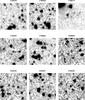 |
Fig. A.1 Images of the reliable (i.e., reliability >90%) counterparts of IFRSs identified in CDFS, ELAIS-S1, and ELAIS-N1 fields. Also reported are the counterparts for the sources ES0436 and ES0593, which are probably not AGN-driven as their R3.6 are around 57. All the images are ~40″ × 40″ wide, North is up and East on the left. The (inverted colours) black-and-white background images are SERVS cutouts, taken from the 3.6 or the 4.5 μm mosaics (depending on which band the reliability has been computed). Superimposed are a red cross (marking the radio peak position, always at the centre of the cutout), and a cyan circle (marking the area within which aperture photometry was derived). |
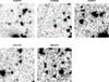 |
Fig. A.1 continued. |
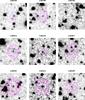 |
Fig. A.2 Images of the reliable (i.e., reliability >90%) counterparts of IFRSs identified in LH SERVS field. All the images are ~40″ × 40″ wide, North is up and East on the left. The (inverted colours) black-and-white background images are SERVS cutouts, taken from the 3.6 or the 4.5 μm mosaics (depending on which band the reliability has been computed). Superimposed are a red cross (marking the radio peak position, always at the centre of the cutout), a cyan circle (marking the area within which aperture photometry was derived), and a green square (marking the position of the optical counterparts, see Table B.1). Also reported are the isophotes of the radio sources (magenta lines, contour levels at 10, 20, 40, 80, 160, 320, 640, and 1280σ the radio image noise). |
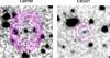 |
Fig. A.2 continued. |
Appendix B: Additional table
Radio and IR properties of the candidate IFRSs in SERVS fields.
All Tables
Main parameters of the radio, SWIRE, and SERVS surveys, together with the number of 1st generation IFRSs identified in each SWIRE and SERVS 3.6 μm field.
Statistics of IFRSs in the SERVS fields as a function of radio-to-IR flux ratio (R3.6).
All Figures
|
Fig. 1 1.4 GHz-to-3.6 μm flux density ratios versus 1.4 GHz radio flux density. The diagonal solid line marks the lowest R3.6 values we can trace due to the combined radio and SERVS detection limits (derived assuming S1.4 GHz > 100 μJy and S3.6 μm > 1 μJy, i.e., the smallest lower limit we measure in our sample). The dotted lines indicate flux density ratios R3.6 = 100, 200, and 500. Flux ratios for reliably IR-detected IFRSs are reported as crosses (position with errors bars), while flux ratios of IR undetected/unreliable sources are indicated by triangles (lower limits). To each field corresponds a different colour, as explained in the legend. |
| In the text | |
|
Fig. 2 Expected flux densities versus redshift for our models: Type 2 and Type 1 AGNs (dotted black and long-dashed grey tracks, respectively); Type 2 and Type 1 QSOs (triple dot-dashed orange and dot-dashed magenta tracks, respectively); radio galaxies (long-dashed green for high-power and dark green for low-power tracks); Arp 220, without and with reddening (dotted cyan and solid blue tracks, respectively), Mrk 231 (dashed red track), and I19254 (long-dashed brown track). Superimposed are the Collier et al. (2014) and Herzog et al. (2014) IFRSs with measured redshift (empty diamonds and empty squares, respectively). Panel a) – Top: IR fluxes at 3.4 (WISE)/3.6 (SWIRE) μm versus redshift; the dashed horizontal line represents the 30 μJy flux density threshold used by Collier et al. (2014) and Herzog et al. (2014) to select their IFRS samples, while the solid horizontal line represents the largest flux density measured in our sample (LH2633, S3.6 μm~5.43 μJy). Panel b) – Bottom: 1.4 GHz radio flux density versus redshift; high-power Type 2 QSO and RLG trends are superimposed due to the identical modelling we applied, as well as for Type 1 AGN and low-power type 1 QSO, and for Type 2 AGN and low-power Type 2 QSO (see Table 4). The dashed horizontal line indicates the lowest 1.4 GHz flux density measured in Collier et al. (2014) and Herzog et al. (2014) samples (7.98 mJy, see Sect. 1), while the solid horizontal line indicates the lowest 1.4 GHz flux density measured in our sample (ES0463, S1.4 GHz~0.14 mJy, see Table B.1). |
| In the text | |
|
Fig. 3 R3.6 ratio evolutionary tracks; in this plot each track is truncated at the redshift at which the radio flux density drops below the detection limit S1.4 GHz ~ 100 μJy. The horizontal dashed lines indicate R3.6 ratios of 100, 200, and 500. The errors associated to the measured R3.6 ratios of the Collier et al. (2014) and Herzog et al. (2014) samples are of the same magnitude of the symbols reported in the plot, and not shown. At the end of the Arp 220 reddened track we indicate the star formation rate expected for this source if it were at redshift ~3, under the hypothesis that star-forming activity entirely accounts for the radio emission in this object. |
| In the text | |
|
Fig. 4 S4.5 μm/S3.6 μm ratios versus 1.4 GHz flux density for IFRS sources. Sources detected only at one IR band (either 3.6 or 4.5 μm), are indicated by the corresponding upper or lower limits. The dashed horizontal lines refer to S4.5 μm/S3.6 μm ratios equal to 1.0, 1.5, and 2.0 respectively. The superimposed tracks refer to HP Type 2 and 1 QSOs (triple dot-dashed orange and dot-dashed magenta respectively), HP RLGs (long-dashed green), Type 1 and 2 AGNs (dashed and dotted grey, respectively), and reddened Arp 220 (solid blue). The redshift increases along the tracks toward the left-hand side of the plot; unitary increments in redshift are marked by dots, starting from the value reported near the first dot on each track. LP QSOs would show a similar track to HP QSOs, but slightly shifted to the left, and are not shown. All the tracks have been drawn in the redshift range within which R3.6 > 50, which is close to the smaller value we measured for our IFRSs (see Table B.1). Empty diamonds and empty squares represent the positions of the IFRSs with redshift from Collier et al. (2014) and Herzog et al. (2014), respectively. In the top-right corner of the plot are shown the median errors for these two samples. Upward empty and filled triangles indicate IFRSs from our sample with R3.6> 500 and between 200 and 500, respectively. The two radio-faintest sources are ES0593 and ES0436, both with R3.6 values below 100. None of the reliably identified IFRSs shown in this plot has R3.6 between 100 and 200. |
| In the text | |
|
Fig. A.1 Images of the reliable (i.e., reliability >90%) counterparts of IFRSs identified in CDFS, ELAIS-S1, and ELAIS-N1 fields. Also reported are the counterparts for the sources ES0436 and ES0593, which are probably not AGN-driven as their R3.6 are around 57. All the images are ~40″ × 40″ wide, North is up and East on the left. The (inverted colours) black-and-white background images are SERVS cutouts, taken from the 3.6 or the 4.5 μm mosaics (depending on which band the reliability has been computed). Superimposed are a red cross (marking the radio peak position, always at the centre of the cutout), and a cyan circle (marking the area within which aperture photometry was derived). |
| In the text | |
|
Fig. A.1 continued. |
| In the text | |
|
Fig. A.2 Images of the reliable (i.e., reliability >90%) counterparts of IFRSs identified in LH SERVS field. All the images are ~40″ × 40″ wide, North is up and East on the left. The (inverted colours) black-and-white background images are SERVS cutouts, taken from the 3.6 or the 4.5 μm mosaics (depending on which band the reliability has been computed). Superimposed are a red cross (marking the radio peak position, always at the centre of the cutout), a cyan circle (marking the area within which aperture photometry was derived), and a green square (marking the position of the optical counterparts, see Table B.1). Also reported are the isophotes of the radio sources (magenta lines, contour levels at 10, 20, 40, 80, 160, 320, 640, and 1280σ the radio image noise). |
| In the text | |
|
Fig. A.2 continued. |
| In the text | |
Current usage metrics show cumulative count of Article Views (full-text article views including HTML views, PDF and ePub downloads, according to the available data) and Abstracts Views on Vision4Press platform.
Data correspond to usage on the plateform after 2015. The current usage metrics is available 48-96 hours after online publication and is updated daily on week days.
Initial download of the metrics may take a while.