| Issue |
A&A
Volume 596, December 2016
|
|
|---|---|---|
| Article Number | A78 | |
| Number of page(s) | 24 | |
| Section | Extragalactic astronomy | |
| DOI | https://doi.org/10.1051/0004-6361/201628974 | |
| Published online | 02 December 2016 | |
Optical polarization of high-energy BL Lacertae objects⋆
1 Aalto University Metsähovi Radio Observatory, Metsähovintie 114, 02540 Kylmälä, Finland
e-mail: This email address is being protected from spambots. You need JavaScript enabled to view it.
2 Aalto University Department of Radio Science and Engineering, PO Box 13000, 00076 Aalto, Finland
3 Tuorla Observatory, Department of Physics and Astronomy, University of Turku, 20014 Turun yliopisto, Finland
4 Department of Physics and Institute of Theoretical and Computational Physics, University of Crete, 71003 Heraklion, Greece
5 Foundation for Research and Technology – Hellas, IESL, Voutes, 71110 Heraklion, Greece
6 Astronomical Institute, St. Petersburg State University, Universitetsky pr. 28, Petrodvoretz, 198504 St. Petersburg, Russia
7 Finnish Centre for Astronomy with ESO (FINCA), University of Turku, 20014 Turun yliopisto, Finland
8 Max-Planck-Institut für Radioastronomie, Auf dem Hügel 69, 53121 Bonn, Germany
9 Nordic Optical Telescope, Apartado 474, 38700 Santa Cruz de La Palma, Santa Cruz de Tenerife, Spain
Received: 20 May 2016
Accepted: 30 August 2016
Abstract
Context. We investigate the optical polarization properties of high-energy BL Lac objects using data from the RoboPol blazar monitoring program and the Nordic Optical Telescope.
Aims. We wish to understand if there are differences between the BL Lac objects that have been detected with the current-generation TeV instruments and those objects that have not yet been detected.
Methods. We used a maximum-likelihood method to investigate the optical polarization fraction and its variability in these sources. In order to study the polarization position angle variability, we calculated the time derivative of the electric vector position angle (EVPA) change. We also studied the spread in the Stokes Q/I−U/I plane and rotations in the polarization plane.
Results. The mean polarization fraction of the TeV-detected BL Lacs is 5%, while the non-TeV sources show a higher mean polarization fraction of 7%. This difference in polarization fraction disappears when the dilution by the unpolarized light of the host galaxy is accounted for. The TeV sources show somewhat lower fractional polarization variability amplitudes than the non-TeV sources. Also the fraction of sources with a smaller spread in the Q/I−U/I plane and a clumped distribution of points away from the origin, possibly indicating a preferred polarization angle, is larger in the TeV than in the non-TeV sources. These differences between TeV and non-TeV samples seem to arise from differences between intermediate and high spectral peaking sources instead of the TeV detection. When the EVPA variations are studied, the rate of EVPA change is similar in both samples. We detect significant EVPA rotations in both TeV and non-TeV sources, showing that rotations can occur in high spectral peaking BL Lac objects when the monitoring cadence is dense enough. Our simulations show that we cannot exclude a random walk origin for these rotations.
Conclusions. These results indicate that there are no intrinsic differences in the polarization properties of the TeV-detected and non-TeV-detected high-energy BL Lac objects. This suggests that the polarization properties are not directly related to the TeV-detection, but instead the TeV loudness is connected to the general flaring activity, redshift, and the synchrotron peak location.
Key words: polarization / BL Lacertae objects: general / galaxies: jets
The polarization curve data are only available at the CDS via anonymous ftp to cdsarc.u-strasbg.fr (130.79.128.5) or via http://cdsarc.u-strasbg.fr/viz-bin/qcat?J/A+A/596/A78
© ESO, 2016
1. Introduction
BL Lac objects are a type of active galactic nuclei characterized by weak or absent emission lines (Stocke et al. 1991). They are typically bright and highly variable at all wavelengths from radio to very high-energy (VHE) gamma rays. Their spectral energy distribution (SED) consists of two humps, the first due to synchrotron radiation, peaking at optical to X-ray wavelengths, and the second due to inverse Compton or some hadronic process, peaking at gamma-ray energies (e.g., Böttcher et al. 2013).
Traditionally, BL Lac objects were classified as radio or X-ray selected based on the wavelength where they were first discovered (e.g., Stickel et al. 1991; Stocke et al. 1991). Padovani & Giommi (1995) refined the classification based on the location of their synchrotron peak to low- and high-peaking BL Lac objects. In this paper we use the classification from the 3rd Fermi Gamma-Ray Space Telescope (hereafter Fermi) AGN catalog (3LAC; Ackermann et al. 2015); in this catalog the sources with synchrotron peak frequency νp< 1014 Hz are called low synchrotron peaked (LSP), sources with 1014<νp< 1015 Hz are intermediate synchrotron peaked (ISP), and sources with νp> 1015 Hz are high synchrotron peaked (HSP).
Another characteristic of BL Lacs is their high and variable optical polarization (e.g., Angel & Stockman 1980; Stocke et al. 1985). The typical polarization fraction of BL Lacs is 5−10% (e.g., Angel & Stockman 1980; Smith et al. 2007; Heidt & Nilsson 2011) with a duty cycle of high polarization (p ≥ 4%) varying from ~40 to 70% depending on the study.
BL Lac objects are also the most numerous extragalactic source class detected in the VHE (>100 GeV) energies according to the TeVCat catalog1 of sources detected by TeV instruments. This prevalence is especially true for the ISP and HSP-type BL Lacs, and can be explained by their high synchrotron peak frequencies, which also shift their high-energy SED peak to higher energies, thereby making them more easily detectable at TeV energies. They are also typically located at relatively low redshifts so that their high-energy emission is not greatly attenuated by the extragalactic background light (EBL). However, many of the sources show featureless spectra making it very difficult to determine their redshifts and the amount of EBL attenuation.
Apart from the location of their SED peaks, it is still unclear what makes an object TeV loud. It seems to be connected to optical (Reinthal et al. 2012; Aleksić et al. 2015; Ahnen et al. 2016a) and GeV (Aleksić et al. 2014) flaring activity, indicating that all ISP and HSP sources could be detected at very high energies if observed during a high flux state. In this paper we study the role of optical polarization variability by comparing a complete sample of TeV-detected BL Lacs with a sample of BL Lacs that are not detected in VHE bands. We concentrate on the ISP and HSP sources as the true nature of the LSP BL Lacs and their classification as BL Lacs is uncertain (e.g., Giommi et al. 2012). We use data from the RoboPol blazar monitoring program (Pavlidou et al. 2014), where a total number of 88 BL Lac objects have been observed. Additionally, we use data of the high-energy BL Lac objects obtained at the Nordic Optical Telescope as a part of a BL Lac monitoring program (PI E. Lindfors).
Our paper is constructed as follows: in Sect. 2 we describe our sample selection and the observations used in this paper. The results from our analysis of the optical polarization fraction and position angle variability are given in Sect. 3. Our discussion and conclusions are described in Sects. 4 and 5. In all the statistical tests we use a limit p = 0.05 as the acceptance limit.
2. Sample and observations
We selected our TeV-detected sample from the TeVCat catalog in January 2014; this sample includes 32 ISP and HSP BL Lacs north of declination 0°, detected by the TeV instruments before 2014. Our TeV sample sources, for which we have reliable polarization measurements (29 objects), are tabulated in Table 1.
In addition to the TeV sample, we constructed a sample of ISP and HSP BL Lac objects that have not been detected by the TeV instruments. The observing strategies of the current-generation TeV instruments result in a biased set of TeV-detected objects, as pointed observations are typically carried out only when the sources are flaring at some other wavelength (e.g., Reinthal et al. 2012). In order to verify that our non-TeV sources are indeed faint in the TeV bands, we took advantage of the second Fermi high-energy catalog 2FHL (Ackermann et al. 2016), which due to its all-sky nature does not suffer from similar selection effects. We used the highest energy band of 171–585 GeV in 2FHL and selected all ISP and HSP objects from the RoboPol main program sample (Pavlidou et al. 2014) that are not detected in this energy bin. This way our non-TeV sample selection is not affected by the pointing strategies of the TeV instruments, and they have a similar observing cadence as our TeV-detected sources. Our non-TeV sample includes 19 objects tabulated in Table 2. Three of these objects have been targeted by the VERITAS telescope with short exposure times, but none of them showed signals higher than 0.3σ (Archambault et al. 2016).
2.1. Redshift distribution
The redshift distributions of the TeV and non-TeV sample sources are shown in Fig. 1. The mean redshift for the TeV sources (0.222 ± 0.035) is smaller than for the non-TeV sources (0.446 ± 0.070). Because of the lower limits, the means were estimated through a Kaplan-Meier estimator implemented in the ASURV package (Lavalley et al. 1992). Similarly, we use the Gehan generalized Wilcoxon test from the ASURV package to estimate the probability that the distributions come from the same population. The test gives p = 0.01, indicating that the non-TeV sources are at higher redshifts, assuming that the lower limits are accurate. This redshift difference affects the TeV detection of the sources, as the EBL attenuation factor for a redshift of 0.45 at 200 GeV is about three times higher than for a redshift of 0.2, albeit still less than one (Franceschini et al. 2008; Domínguez et al. 2011). However, considering the recent detections of TeV emission from objects at z> 0.9 by the MAGIC telescopes (Sitarek et al. 2015; Ahnen et al. 2015), it is likely that this is not the only reason why the sources are not detected by the TeV instruments.
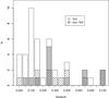 |
Fig. 1 Stacked histogram of the redshift in the TeV (white) and non-TeV (gray) samples. The hatched bars show the fraction of sources with lower limit redshifts. |
TeV sample sources and their variability properties.
Non-TeV sample sources and their variability properties.
2.2. SED classification
There are several ways to model the SEDs of blazars, for example, by using a parabolic fit (e.g., Nieppola et al. 2006), a third degree polynomial fit (e.g., Ackermann et al. 2015), or an empirical relation between the radio-optical and optical-X-ray spectral indices (e.g., Ackermann et al. 2011) . In BL Lac objects the host galaxy contribution in the optical band may also shift the peak frequency to a lower value, depending on how the fit is carried out. For example, VER J0521+211 in our TeV sample is classified as HSP in TeVCat, while it is listed as an ISP in the 3LAC catalog. We take all our SED classifications from 3LAC (Ackermann et al. 2015), where they have been uniformly estimated for both of our samples. Our TeV sample includes only three ISP sources, while these form the majority (13/19) of the non-TeV sample. Sometimes the sources are also seen to change their SED peak frequency during flaring (e.g., Pian et al. 1998; Giommi et al. 2000; Ahnen et al. 2016b), which further complicates the classification. Thus, it is clear that our TeV and non-TeV samples differ in their SED properties, which along with the redshift difference may explain why the non-TeV objects have not been detected at TeV energies. Therefore, whenever possible, we check how the SED classification difference affects our results.
2.3. RoboPol observations
Optical R-band polarization observations were obtained for the TeV and and non-TeV sources with the RoboPol instrument, mounted on the 1.3 m telescope at Skinakas Observatory2 in Crete. The polarimeter contains a fixed set of two Wollaston prisms and half-wave plates, allowing simultaneous measurements of the Stokes I,Q/I,U/I parameters for all point sources within the 13′ × 13′ field. The R-band magnitudes were calculated using calibrated field stars either from the literature3 or from the Palomar Transient Factory R-band catalog (Ofek et al. 2012) or the USNO-B1.0 catalog (Monet et al. 2003), depending on their availability. The exposure time was adjusted based the brightness of the target and sky conditions, and varied between 100 s and 1800 s.
The observations were reduced using the pipeline described in King et al. (2014), which uses aperture photometry. The TeV sources were measured with a fixed 3″ aperture diameter. In the non-TeV sources where the host galaxy contribution is smaller (see Sect. 3.2), to optimize the S/N, the aperture size was defined as 2.5 × FWHM, where FWHM is an average full width at half maximum of stellar images. The average FWHM for RoboPol images is equal to 2.07″. The stability of the instrumental polarization was controlled by nightly observations of polarized and zero-polarized standard stars.
Four sources, 1ES 0033+595, 1ES 1440+122, Mrk 421 and 1ES 1741+196, had confusing field sources entering the aperture, preventing us from obtaining good quality observations with RoboPol. In addition, three sources, 1ES 0229+200, Mrk 501, and 1ES 2344+514, had a host galaxy that was too bright for reliable polarization measurements with RoboPol. Consequently, Mrk 421 and Mrk 501 were excluded from our sample, while for the other four problematic cases we have observations taken with the Nordic Optical Telescope (see below).
All the non-TeV sources and some of the TeV sources were already part of the RoboPol main monitoring sample (Pavlidou et al. 2014), while others were added into the monitoring as a separate TeV-source project. We only use data taken during the 2014 observing season, which lasted from April to November. The mean number of observations for the TeV sources is 9.6 and for the non-TeV sources 10.8. These are also tabulated for each individual source in Tables 1 and 2.
2.4. Nordic optical telescope observations
We also obtained observations with the Nordic Optical Telescope (NOT)4 for 13 TeV sources. The observations of 1ES 0033+595 had to be excluded from the analysis because of a close-by confusing source, bringing our final TeV-detected sample to 29 sources.
The observations were carried out with ALFOSC5 in the R band using the standard setup for linear polarization observations (lambda/2 retarder followed by a calcite). The observations were performed twice per month from April 2014 to November 2014. In total we had 15 observing epochs. The exposure times varied from 10 s to 360 s depending on the source brightness. Polarization standards were observed monthly to determine the zero point of the position angle. The instrumental polarization was determined using observations of zero polarization standard stars and was found to be negligible. The observations were mostly conducted under good (~1″) seeing conditions.
The data were analyzed using the pipeline developed at the Tuorla Observatory. This pipeline uses standard procedures with semi-automatic software. The sky-subtracted target counts were measured in the ordinary and extraordinary beams using aperture photometry. The normalized Stokes parameters and the polarization fraction and position angle were calculated from the intensity ratios of the two beams using standard formula (e.g., Landi Degl’Innocenti et al. 2007). As the data were taken under good seeing conditions, and the optics of NOT are excellent, we were able to use aperture diameter of 3″ to minimize the contribution of the unpolarized host galaxy flux to our measurements.
Because the field of view in our observations is rather small, and in many cases includes no comparison stars to be used for differential photometry, we were only able to perform photometry for the NOT data of 1ES 2344+514.
3. Results
We show the polarization time series of all sources in Appendix A.
3.1. Polarization fraction and its variability
Here we examine whether the mean polarization fraction and its variability amplitude are different for the TeV and non-TeV samples. We used a maximum-likelihood approach to estimate the “intrinsic” mean polarization fraction and modulation index (standard deviation over mean) of the source. The term “intrinsic” denotes values we would expect if we had perfect sampling and no measurement uncertainties. We assumed the polarization fraction follows a Beta distribution because Beta distribution is confined between 0 and 1 similarly as the polarization fraction. We accounted for the observational uncertainties by convolving the probability density of the Beta distribution with a probability density of the Ricean distribution (assumed distribution for a single polarization measurement). This results in a probability density function  (1)where p is the polarization fraction and α and β determine the shape of the Beta distribution B(α,β). If the parameters a,β of this distribution are known, the mean polarization fraction and the intrinsic modulation index are then given by
  (2)and
  (3)where Var is the variance of the distribution. Details of the method are described in the appendix A of Blinov et al. (2016).
The main advantage of this method is that it provides uncertainties for both the mean polarization fraction and the modulation index, and when the values cannot be constrained, it is possible to calculate a 2σ upper limit. One important thing to note is that the method takes the observed polarization fraction without debiasing as input, and automatically and properly accounts for biasing (for details on why debiasing is typically applied, see, e.g., Simmons & Stewart 1985). For this reason, the polarization curves presented in Appendix A do not have debiasing applied.
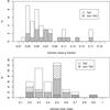 |
Fig. 2 Top: stacked histogram of the intrinsic mean polarization fraction in the TeV (white) and non-TeV (gray) samples. Bottom: stacked histogram of the intrinsic modulation index in the TeV (white) and non-TeV (gray) samples. The hatched bars show the fraction of TeV or non-TeV sources that have only 2σ upper limits available. |
The likelihood method is applicable to sources with at least three observations out of which at least two have a signal-to-noise ratio ≥3. This results in a sample of 25 TeV and 17 non-TeV sources. The mean polarization fraction and the intrinsic modulation index are tabulated in Table 1 for the TeV sources and in Table 2 for the non-TeV sources.
In Fig. 2 (top panel) we show the distribution of the intrinsic mean polarization fraction for the TeV and non-TeV samples. The mean polarization fraction for the TeV sources is 0.054 ± 0.008 and for the non-TeV sources 0.073 ± 0.009. A two-sample Kolmogorov-Smirnov (K-S) test gives a p value of 0.070 for the null hypothesis that the two samples were drawn from the same distribution, so the null hypothesis cannot be rejected on the grounds of that test. However, a two-sided Wilcoxon test gives a probability of p = 0.028 that the means of the distributions are the same, which indicates that the non-TeV sources have higher intrinsic polarization fraction than the TeV sources.
The bottom panel of Fig. 2 shows the distributions for the intrinsic modulation index. Because of the upper limits, we calculated the means of the distributions through a Kaplan-Meier estimate, which gives 0.29 ± 0.03 for the TeV sources and 0.38 ± 0.04 for the non-TeV sources. The Gehan generalized Wilcoxon test gives a probability of p = 0.031 that the two distributions come from the same population, indicating that the non-TeV sources are more variable than the TeV sources. If we only consider the HSP sources, the two samples can no longer be distinguished (p = 0.71) and the mean values are more similar (0.31 ± 0.03 for the TeV and 0.36 ± 0.09 for the non-TeV sources). However, our sample includes only five HSP non-TeV sources for which we obtained a modulation index so that the result is affected by the small number of sources.
3.2. Host galaxy contribution
The host galaxies of TeV blazars are known to contribute significantly (Nilsson et al. 2007) and it is therefore possible that our polarization fraction observations are affected by the unpolarized starlight from the galaxy (e.g., Andruchow et al. 2008; Heidt & Nilsson 2011). In order to test this, we collected host galaxy magnitudes for the sources in our sample from the literature. These are tabulated in Tables 1 and 2 along with the observed and Galactic extinction-corrected magnitudes. We used the recalibrated dust maps of Schlafly & Finkbeiner (2011) with the reddening law of Fitzpatrick (1999) extracted from NASA/IPAC Extragalactic Database (NED) for the Galactic extinction correction.
Most of the host galaxy magnitude estimates in the literature are obtained by modeling the core and galaxy emission using a De Vaucouleurs intensity profile integrated to infinity (e.g., Nilsson et al. 1999). In these cases, whenever the effective radius of the galaxy was available in the literature, we estimated the contribution of the host galaxy to our magnitude estimates by integrating up to the aperture size used in our observations, using the equations described in Nilsson et al. (2009). As explained in Sect. 2.3, we used a different aperture size for the TeV and non-TeV sources. Therefore, for the TeV sources, we integrated up to a radius of 1.5″, and for the non-TeV sources, we used an aperture radius of 2.6″.
If the host galaxy magnitude or limit was not obtained using an R-band filter, we converted between the magnitude systems using the following average color relations for elliptical galaxies from Kotilainen et al. (1998) and Fukugita et al. (1995): R−H = 2.5, H−K = 0.2, and R−I = 0.7. In Shaw et al. (2013b), the absolute magnitude of the host galaxy is estimated from the spectra instead of fitting images. We converted their absolute magnitudes to apparent magnitudes using the cosmological parameters listed in their paper. The values tabulated in Tables 1 and 2 are the R-band host magnitude values we use in our analysis while we reference the original paper where the host magnitude is given. Ideally, one should use the same aperture size and same calibration stars as in the original derivation of the host magnitude to obtain accurate results. As this is not possible for most of our sources, the uncertainty in the host-corrected magnitudes is most likely very large and values for individual sources should be treated with caution.
In the following we only consider sources for which we were able to determine a mean polarization fraction using the likelihood analysis. As explained in Sect. 2.4, owing to the small field of view of the NOT polarimeter and the lack of calibrated standard stars in the field, we were only able to estimate photometry for 1ES 2344+514 from our NOT observations. We tabulated the mean magnitudes for the sources without NOT magnitudes using data from the Tuorla blazar monitoring program6 (Takalo et al. 2008) taken in 2014 but do not use them in the following analysis.
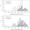 |
Fig. 3 Top: stacked histogram of the extinction-corrected mean magnitude in the TeV (white) and non-TeV (gray) samples. Bottom: stacked histogram of the host-corrected mean magnitude in the TeV (white hatched) and non-TeV (gray hatched) samples. For sources where a host correction is not available, we show the extinction-corrected mean magnitudes as in the top panel. |
In Fig. 3 top panel we show the extinction-corrected magnitudes for the TeV and non-TeV samples. The outlier TeV source in the figure is the extreme HSP source HESS J1943+213 (Akiyama et al. 2016; Straal et al. 2016) at a low Galactic latitude where the extinction correction is uncertain. Therefore we exclude it from the statistical tests; we note that the conclusion remains the same regardless of its exclusion. The mean extinction-corrected magnitude for the TeV sources is 15.2 ± 0.2 and for the non-TeV sources 16.4 ± 0.2. A K-S test gives p = 0.004 for the distributions to come from the same population, which indicates that our TeV and non-TeV sources have different magnitude distributions, which is not surprising considering that the non-TeV sources reside at higher cosmological distances. Because the TeV sources are much brighter in the optical than the non-TeV sources, they may also be brighter in the gamma-ray bands as the fluxes of BL Lac objects in these two regimes are correlated (e.g., Bloom et al. 1997; Hovatta et al. 2014; Wierzcholska et al. 2015). This may in part also explain why some objects in our non-TeV sample are not detected at TeV energies with the current instruments.
The bottom panel of Fig. 3 shows the host- and extinction-corrected magnitudes in the hatched bars for the sources where a host galaxy magnitude was found in the literature. Combining the host- and extinction-only-corrected (where host correction is not available) magnitudes, the TeV sources have a mean magnitude of 15.4 ± 0.2 and the non-TeV sources a mean magnitude of 16.4 ± 0.2. A K-S test gives p = 0.043, which indicates that even when the host correction is accounted for, the non-TeV sources are fainter. We have a host magnitude estimate for only two non-TeV sources and, in both cases, the magnitude changes only very little, so that the non-TeV sample mean is very similar to the uncorrected sample. The lack of host magnitude estimates for the non-TeV sources is likely because the sources reside at higher redshifts than the TeV sources. In fact, many of these sources were observed by Shaw et al. (2013b), but no host galaxy contribution was seen in their spectra. Considering the strong dependence of the host galaxy luminosity on redshift (Nilsson et al. 2003), we can expect the host galaxy contribution in the remaining non-TeV sources to be small.
We then proceed to estimate the amount of unpolarized host-galaxy light on our polarization fraction estimates. We remove the host galaxy flux density from the mean observed flux density and recalculate the host-corrected polarization fraction pcorr following, 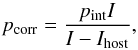 (4)where pint is the mean polarization fraction from the likelihood analysis, I is the flux density calculated from the mean observed magnitude, and Ihost is the flux density of the host galaxy.
We find that the mean polarization fraction in the TeV sample is 0.068 ± 0.010, which is similar (K-S test p = 0.345) as in the non-TeV sample where the mean is 0.073 ± 0.009. This indicates that after correcting for the host galaxy contribution, the polarization fraction of the TeV and non-TeV samples cannot be distinguished.
3.3. Polarization angle variability
In this section we examine whether there are differences in the polarization angle variability of the TeV and non-TeV samples. We do this first by calculating the time derivative of the electric vector position angle (EVPA). We smooth the EVPA curves by always requiring that the difference between consecutive points is <90° to account for the nπ ambiguity in the position angle. We only use observations with a signal-to-noise ratio of at least three in the polarization fraction. In calculation of the derivative, we further require that the change in the EVPA between consecutive points meets the following criteria: ![Mathematical equation: \begin{equation} |\theta[i+1]-\theta[i]| > \sqrt{\sigma[i+1]^2+\sigma[i]^2}, \end{equation}](/articles/aa/full_html/2016/12/aa28974-16/aa28974-16-eq217.png) (5)where θ is the EVPA and σ its uncertainty. If this criterion is not met, we can either set the derivative to zero or ignore it. The first way is more appropriate when the sources do not exhibit much variation, while the latter gives an estimate of the typical rate in the polarization angle variability when they do change significantly. In both cases we calculate the derivative between two consecutive points and take the absolute value. For sources with a redshift estimate or limit available, we multiply the observed derivative by (1 + z) to look at the variations in the source frame. We use the redshift limits as values when doing this. For sources without redshift estimates, we do not correct the derivative.
(5)where θ is the EVPA and σ its uncertainty. If this criterion is not met, we can either set the derivative to zero or ignore it. The first way is more appropriate when the sources do not exhibit much variation, while the latter gives an estimate of the typical rate in the polarization angle variability when they do change significantly. In both cases we calculate the derivative between two consecutive points and take the absolute value. For sources with a redshift estimate or limit available, we multiply the observed derivative by (1 + z) to look at the variations in the source frame. We use the redshift limits as values when doing this. For sources without redshift estimates, we do not correct the derivative.
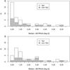 |
Fig. 4 Stacked histogram of the median EVPA derivative for the TeV (white) and non-TeV (gray) samples. Top panel: shows the distribution when the derivative is set to zero for insignificant changes and the bottom panel shows the same when insignificant changes are ignored (see text for details). |
The distribution of the median redshift-corrected absolute derivatives for each source are shown in Fig. 4. The top panel shows the distributions when the derivative is set to zero for insignificant changes. The mean values of the distributions are similar for the TeV (mean 1.11 ± 0.29) and non-TeV (mean 1.66 ± 0.45) samples. A K-S test gives a probability p = 0.583 for these samples to come from the same population. If we look at the HSP non-TeV sources only (five sources), their mean is 0.62 ± 0.31, which is similar to the TeV mean.
The bottom panel shows similar distributions when ignoring derivatives between insignificant variations. As expected, the mean values are now higher (TeV mean 1.81 ± 0.39 and non-TeV mean 2.38 ± 0.40) and in this case the K-S test gives a probability p = 0.034, indicating that the magnitude is larger in non-TeV sources when the sources show significant variability between consecutive measurements. The true difference could be even larger as many of the non-TeV sources do not have redshift estimates available. Again, if we only consider the HSP non-TeV sources, the mean is 1.71 ± 0.55, very close to the TeV source mean.
Another way to study the polarization angle variability is to look at the polarization in the Q/I–U/I plane. The Q/I–U/I plots for each individual source are shown in Appendix A. A larger spread in the Q/I−U/I plane suggests more EVPA variability, while a clumped distribution away from the origin could be an indication of a preferred polarization angle. We calculate the weighted mean Q/I and U/I as the mass center of the points to quantify these effects. The distribution of the distance of the mass center from origin is shown in Fig. 5 top panel. The mean distance for the TeV sources is 0.050 ± 0.008 and for the non-TeV sources 0.060 ± 0.010. As expected, these are similar to the intrinsic mean polarization degree estimates. A K-S test gives p = 0.197 for the distributions to come from the same population, and we cannot reject the null hypothesis.
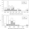 |
Fig. 5 Top: stacked histogram of the distance of the mass center in the Q/I−U/I plane from the origin. Bottom: stacked histogram of the mean distance of the Q/I vs. U/I points from the mass center. The TeV sources are shown in white and non-TeV sources in gray. |
We then estimate the distance of each individual measurement to this mass center, and take a mean value to estimate the scatter in the Q/I−U/I plane. The distributions of these mean distances are shown in Fig. 5 bottom panel for both the TeV and non-TeV samples. The mean value for the TeV sources is 0.021 ± 0.003 and for the non-TeV sources 0.041 ± 0.005. According to a K-S test, which gives p = 0.003, we can reject the null hypothesis that these come from the same population, indicating that the TeV sources show less spread in the Q/I−U/I plane. This is in accordance with the modulation index results where the TeV sources were found to show less variability than the non-TeV sources.
4. Discussion
Our aim was to study the differences in the TeV-detected ISP and HSP BL Lac objects compared to non-TeV-detected objects. In this study we have compared the optical polarization properties of a TeV-detected sample of 29 sources with a sample of 19 non-TeV objects. Our maximum-likelihood analysis shows that there are no differences in the mean polarization fraction in the two samples, indicating that optical polarization variability and the TeV emission are not directly related. Instead, their redshift distributions, SED classifications, and optical brightness are seen to differ significantly, which most likely explains why some of these sources are TeV detected while others are not. In the following sections we compare our results to earlier studies and analyze the polarization angle behavior in more detail.
4.1. Fraction of polarized sources and the duty cycle of high polarization
Optical polarization of X-ray-selected BL Lac objects was studied by Jannuzi et al. (1994) who examined three years of optical polarization monitoring data. They detected significant polarization in 28 out of 37 sources, out of which 19 showed significant variability. We detected polarization at a level of signal-to-noise greater than three in all but one TeV (RBS 0413) and non-TeV (SBS 1200+608) source showing that our detection fraction is higher (46 out of 48 sources). We detect significant variability in 17 TeV and 12 non-TeV sources, which makes the fraction of variable sources very similar to Jannuzi et al. (1994).
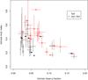 |
Fig. 6 Intrinsic modulation index against the intrinsic mean polarization fraction for the TeV (black circles) and non-TeV (red open squares) sources. Lower limits in modulation index are shown with downward triangles. |
In Fig. 6 we show the intrinsic modulation index against the polarization fraction. There is a trend for sources with higher mean polarization fraction to show smaller polarization variability amplitudes. This could indicate that the sources with higher polarization fractions had a more ordered dominating polarization component. A similar trend is seen when the full RoboPol sample is examined (Angelakis et al. 2016).
Jannuzi et al. (1994) also find that the duty cycle for the fraction of time these sources are highly polarized at >4% is 44%. We calculate the duty cycle in our sample in the same way as these authors by taking the first observation of each source and calculating the fraction of sources that have polarization fraction >4%. In the calculation of the duty cycle, we account for the Ricean bias and debias our polarization fraction observations following Pavlidou et al. (2014). Accounting for the uncertainties in the measurements, we find the duty cycle in our TeV objects to be  and in the non-TeV sources
  , which are consistent with each other within uncertainties. They are higher than obtained by Jannuzi et al. (1994) but similar to Heidt & Nilsson (2011) who found a duty cycle of 66% for HBL BL Lacs.
4.2. Host galaxy dilution
Heidt & Nilsson (2011) suggested that one reason why they obtained a higher duty cycle than Jannuzi et al. (1994) is because of the larger aperture size used by Jannuzi et al. (1994), which would result in a larger portion of the host galaxy contaminating the polarization results. Heidt & Nilsson (2011) also found that sources with known redshifts are less polarized than sources with unknown redshifts, and they found a trend for sources at redshift of ≳1 to be more highly polarized. They suggested this is also due to host galaxy dilution of the polarization fraction as in lower redshift sources, for which the redshift is also easier to determine, the host galaxy contribution within the aperture is larger.
We examined this directly by collecting from the literature all the available host galaxy magnitudes, and correcting our polarization fraction by removing the contribution of the unpolarized host. In Sect. 3.2, we showed that this increases the polarization fraction in the TeV sources, and reduces the difference between the TeV and non-TeV sources. As only 13 of our 19 non-TeV sources have a redshift estimate or limit available, this may also indicate that the redshifts of the remaining non-TeV sources are higher than in our TeV sources, in agreement with the findings of Heidt & Nilsson (2011).
4.3. Preferred polarization angle
Angel et al. (1978) claimed that at least some BL Lac objects have a preferred polarization angle over several years of observations. Jannuzi et al. (1994) found that 11 out of 13 sources in their well-studied sample, with a time span of at least 20 months between the first and last observations, have preferred polarization angles. In Sect. 3.3 we found that the distance of the mass center from the origin was similar in the two samples, while the scatter in the Q/I−U/I plane was significantly smaller for the TeV-detected than the non-TeV samples. If we look at the fraction of sources for which the scatter is smaller than a third of the distance from the origin, i.e., sources far away from the origin with small scatter (an indication of a preferred polarization angle), the fraction of TeV sources is much higher (11/26) than in the non-TeV sources (3/17).
Assuming that these 14 sources have a preferred polarization angle, we can try to estimate the direction of the magnetic field relative to the jet direction by comparing the mean EVPA to the jet position angle. We do this by collecting from the literature the jet position angles of the innermost jet components obtained through Very Long Baseline Interferometry (VLBI). These are available for 9 of the TeV sources and we tabulate them in Table 1. We show the difference of the mean EVPA and the jet position angle in Fig. 7. As the optical emission is optically thin, the projected magnetic field is perpendicular to the observed EVPA direction so that a small difference between EVPA and jet position angle corresponds to magnetic field perpendicular to the jet direction. Relativistic effects may alter the appearance of this distribution, as discussed in Lyutikov et al. (2005), so the situation may not be as straightforward.
Figure 7 shows that 67% of the sources for which both the EVPA and jet position angle are available (six out of nine sources) show a difference of less than 20 degrees, indicating that the magnetic field is perpendicular to the jet direction. A K-S test gives a p = 0.0003 for the sample to come from a uniform distribution. The distribution looks similar to a comparison between optical EVPA and the inner-jet position angle at 43 GHz for a sample of highly polarized quasars (Lister & Smith 2000) and a sample of BL Lac objects (Jorstad et al. 2007). We note a caveat that many of the jet position angle observations are taken at fairly low radio frequencies (8 or 15 GHz). Therefore, the position angle may not be representative of the jet position angle in the optical band, as some blazars are known to show significant curvature in the inner jets (e.g., Savolainen et al. 2006), although for BL Lac objects the alignment at least from 43 GHz to optical seems to be better than in quasars (Jorstad et al. 2007). Our analysis also relies on the assumption that the mean EVPA represents a stable EVPA of the jet, which may not be the case considering the fairly short time span of our observations. As discussed in, for example, Villforth et al. (2010) and Sakimoto et al. (2013), it is also possible that the same sources occasionally show a preferred polarization angle while at another time they may not, so clearly long-term polarization observations are required to better understand this in the HSP objects.
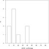 |
Fig. 7 Stacked histogram of the difference between the mean optical EVPA and inner jet position angle from VLBI observations for the TeV sources showing indications of a preferred polarization angle. |
4.4. Scatter in the Q/I – U/I plane
In order to investigate the difference in the scatter between the two samples, in Fig. 8 we show stacked plots for all the TeV (left) and non-TeV (right) sources by shifting the mass center of the individual sources to the origin. While the scatter is larger in the non-TeV than in the TeV sources, this seems to be a difference between HSP and ISP-type objects rather than TeV and non-TeV sources. As discussed in Sect. 2.2, the non-TeV sample contains a much larger percentage of ISP objects than the TeV sample, and the HSP sources in the non-TeV sample have a similar range of scatter in the Q/I−U/I plane as the TeV sources. This agrees with our results in Sect. 3.1 , where we found that the non-TeV sample sources have higher polarization fraction variability amplitudes, and Sect. 3.3 where the rate of EVPA change was found to be larger in the non-TeV sample, but very similar to the TeV sources if we only consider the HSP-type non-TeV sources. Also, when the full RoboPol sample is examined, there is a trend for higher synchrotron peak sources to have more preferred EVPA distributions (Angelakis et al. 2016).
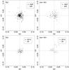 |
Fig. 8 Top: stacked Q/I vs. U/I plot for the TeV (left) and non-TeV (right) samples. Bottom: same for three TeV sources (left) and two non-TeV sources (right) for which we have data over multiple seasons. The stacking is performed by shifting the mass center of each source to the origin. In the bottom panel we stacked the data based on the mass center of all data, which is why the top and bottom panels are not exactly the same for the 2014 data. |
There could be several causes for this. Because we are observing the sources over a fixed band, we probe a different part of the SED in the ISP and HSP sources. This results in larger total intensity variability in the ISPs than in HSPs (e.g., Hovatta et al. 2014) because the optical emission in ISPs is produced by electrons with energies above the synchrotron break frequency, while in HSPs the optical emission is produced by electrons with energies less than the break frequency. Thus, any new emission component changes the total intensity by a larger amount in the ISPs, which could be reflected in the polarization fraction observations, if the polarized flux does not change at a same rate. In this case, we would expect to see more scatter in the HSP sources when observed in X-ray bands, a good test case for the future X-ray polarization missions. This effect is discussed more in Angelakis et al. (2016) where the polarization amplitude variability in the full RoboPol sample including LSP, ISP, and HSP sources is analyzed.
Another alternative could be lower optical Doppler beaming in the HSPs compared to ISPs as might be expected based on radio observations of these objects (e.g., Lister et al. 2011). If the Doppler factor in the HSP sources is lower, it takes a longer time to probe the same range of variability as in the ISP objects. Because we have only used one season of data for these objects, it is possible that the true spread in the Q/I−U/I plane in the HSPs is larger, if we monitor them longer. Some of the TeV sources in our sample are also in the main sample of the RoboPol program, and we can investigate whether inclusion of more data changes the picture. We select three of the HSP TeV sources (RGB J0710+591, Markarian 180, and 1ES 1959+650) with least amount of scatter (mean distance from the mass center <0.2) for which we also have data from 2013 (the first two sources) and 2015 (the last source). Similarly, we select two HSP non-TeV sources (RBS 1752 and 1RXSJ 234051.4+801513) for which we have data from 2013–2015. In Fig. 8 lower panel we show the Q/I−U/I points for these sources with the 2014 points indicated in black symbols and the data from all seasons shown in gray symbols. We can see that the scatter increases when more data from the other seasons are added, showing that longer monitoring time is required to draw strong conclusions about the scatter.
4.5. Rotations in the polarization plane
It is clear that not all the HSP sources have a preferred angle in our analysis and one reason for this could be rotations in polarization plane. Even though EVPA rotations were observed many decades ago (e.g., Kikuchi et al. 1988), for a long time it was unclear whether these rotations are seen in all types of objects and, especially, in HSPs. During the first observing season of RoboPol in 2013, we detected a 128 degree EVPA rotation in the HSP source PG 1553+113 (Blinov et al. 2015). The same source was also seen to rotate by about 145 degrees during 2014, as reported in Blinov et al. (2016), confirming the TeV HSPs as a class of objects with EVPA rotations (see also Jermak et al. 2016).
In this paper, following Kiehlmann et al. (2016) we define an EVPA rotation as a period in which the EVPA continuously rotates in one direction. Insignificant counter-rotations with 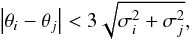 (6)where θi and θj are the first and last data point of the counter-rotation and
  ,
,  the corresponding uncertainties, are not considered to break a continuous rotation. Additionally, we consider only smooth rotations, where each pair of adjacent derivatives does not change by more than 10 degrees per day. We further require that the rotation consists of at least four observations and that the corresponding polarization fraction has a signal-to-noise ratio of at least three.
We find significant rotations in three of the HSP TeV sources (RGB J0136+391, PG 1553+113, and 1ES 1727+502), and nine rotations in six non-TeV sources (GB6 J1037+5711, GB6 J1542+6129, TXS 1557+565, 87GB 164812.2+524023, RXJ 1809.3+2041, and S5 2023+760). These are shown as shaded regions over the EVPA curves in Appendix A. The rotations in PG 1553+113, GB6 J1037+5711, and S5 2023+760 were already reported in Blinov et al. (2016). This shows that EVPA rotations can occur also in ISP and HSP sources if they are observed at high enough cadence. We would not have detected the rotations in RGB J0136+391 and 1ES 1727+502 if we did not have both RoboPol and NOT observations of them. The fraction of rotating sources is much higher in the non-TeV sample, although we note that only one of them is an HSP-type source (RXJ 1809.3+2041), so this could simply reflect the differences in the EVPA variations of the ISP and HSP sources in the optical band. The differences in the number of rotations in LSP, ISP, and HSP sources in the RoboPol sample are studied in Blinov et al. (2016b)
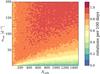 |
Fig. 9 Frequency of rotations per 100 days for various combinations of the number of cells Ncells and number of them nvar that change during each step. |
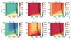 |
Fig. 10 Probability of observing n = 0,1,2 observations during our observing season for the TeV source RGB J0136+391 (top) and the non-TeV source GB6 J1037+5711 (bottom). The color scale shows the probability for a various set of parameters nvar and Ncells. The white dot indicates the best-fit region for obtaining a similar polarization fraction as in the observed light curve and the black curves show its 95% confidence interval. |
We ran a set of simulations to investigate the physical nature behind these rotations. We used the simple Q,U random walk process described in Kiehlmann et al. (2016). Our jet consists of Ncells, each with a uniform magnetic field at a random orientation. During each step of the simulation, we let nvar cells change their magnetic field orientation. For details of the simulation steps, see Kiehlmann et al. (2016).
In our simulations, we probe the range Ncells = [20,40,...,1500] and nvar = [2,4,...,200] and run 500 simulations for each combination. The time sampling of the light curve, length of the season, and the q and u uncertainties are taken from the cumulative distribution function of the real observations. The rotations in the simulations are then identified in the same manner as for the real data. This allows us to calculate the frequency of rotations per 100 days for each parameter set; the result is shown in Fig. 9. We can see that, as expected, the frequency of rotations increases when a larger number of cells change per day, and also that less total number of cells produces more frequently rotations.
We then examine how this relates to the rotations observed in the individual objects. First, based on the expected frequency of rotations λ, we calculate the probability of observing n = 0,1,2 rotations over the model grid using Poisson statistics 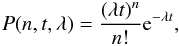 where t is the total length of the season for each source. The only parameter that changes for each source is the season length t. In Fig. 10, we show examples for two of the sources showing rotations RGB J0136+391 (TeV source) and GB6 J1037+5711 (non-TeV source). Because the sampling is fairly uniform across the samples, the results for all individual sources are very similar to the example cases.
We can see that the probability of observing 0, 1, or 2 rotations is non-zero in all cases and at least some parameter combinations are able to produce rotations during our season with high probability. In order to further examine how well the simulated light curves match our observed ones, we find all the simulations where the mean polarization fraction of the simulated light curve is within uncertainties of the observed mean polarization fraction. Here the uncertainties are determined using a bootstrap approach that is similar to Kiehlmann et al. (2016). We then select the region of the parameter space that most likely produces the observed mean polarization fraction. The best-fit value is shown as a white dot in the panels in Fig. 10, and the black lines show the 95% confidence intervals.
For all the sources, the probability of observing a single rotation is between 15 and 37%, which is consistent with our detected number of rotations especially in the non-TeV sources. In TeV sources we see fewer rotations than expected (~10%), which could be due to the sources showing a preferred polarization angle more often, which would hinder us from detecting EVPA rotations. The probability of observing two rotations is much less, although it is not small enough to rule out a random walk process. Even though it is not possible to rule it out for the individual sources, Blinov et al. (2015) showed that it is unlikely that all rotations in the full RoboPol sample are caused by a random walk process. We also note that we have not examined the characteristics of the rotations (e.g., their smoothness), which may further restrict the parameter space where rotations can be observed and help to distinguish between deterministic and stochastic rotations (Kiehlmann et al. 2016; in prep.). Detailed modeling of these rotations along with multifrequency data will be presented elsewhere.
5. Conclusions
We have studied the optical polarization variability in a sample of TeV-detected and non-detected ISP and HSP-type BL Lac objects using data from the RoboPol and NOT instruments. Our main conclusions can be summarized as follows:
-
1.
The mean polarization fraction of the TeV-detectedBL Lacs is 5%, while the non-TeV sourcesshow a higher mean polarization fraction of 7%. This differ-ence in polarization fraction disappears when the dilutionby the unpolarized light of the host galaxy is accounted for.This is a similar polarization fraction as in optically selectedBL Lac objects (e.g., Smithet al. 2007), although an anal-ysis of the full RoboPol sample reveals a negative trend inthe optical polarization fraction as a function of the syn-chrotron peak with LSP sources showing typically a highermean polarization fraction than HSP sources (Angelakiset al. 2016).
-
2.
When the polarization variations are studied, the rate of EVPA change is similar in both samples. The fraction of sources with a smaller spread in the Q/I−U/I plane along with a clumped distribution of points away from the origin, possibly indicating a preferred polarization angle, is larger in the TeV than in the non-TeV sources. We also find that the non-TeV sources show larger polarization fraction variability amplitudes than the TeV sources. This difference between TeV and and non-TeV samples seems to arise from differences between the ISP and HSP-type sources instead of the TeV detection.
-
3.
We detect significant EVPA rotations in both TeV and non-TeV sources, showing that rotations can occur in high spectral peaking BL Lac objects when the monitoring cadence is dense enough. Our simulations show that we cannot exclude a random walk origin for these rotations.
We conclude that TeV loudness is more likely connected to general flaring activity, redshift, and the location of the synchrotron peak rather than the polarization properties of these sources.
Acknowledgments
We thank the referee, P. Giommi, for the careful reading of the paper and suggestions that improved it significantly. T.H. was supported by the Academy of Finland project number 267 324. Part of this work was supported by the COST Action MP1104 “Polarization as a tool to study the Solar System and beyond”. D.B. acknowledges support from the St. Petersburg University research grant No. 6.38.335.2015. I.M. was supported for this research through a stipend from the International Max Planck Research School (IMPRS) for Astronomy and Astrophysics at the Universities of Bonn and Cologne. The data presented here were obtained in part with ALFOSC, which is provided by the Instituto de Astrofisica de Andalucia (IAA) under a joint agreement with the University of Copenhagen and NOTSA. The RoboPol project is a collaboration between the University of Crete/FORTH in Greece, Caltech in the USA, MPIfR in Germany, IUCAA in India and Torún Centre for Astronomy in Poland. The U. of Crete group acknowledges support by the “RoboPol” project, which is co-funded by the European Social Fund (ESF) and Greek National Resources, and by the European Commission Seventh Framework Programme (FP7) through grants PCIG10-GA-2011-304001 “JetPop” and PIRSES-GA-2012-31578 “EuroCal”. This research was supported in part by NASA grant NNX11A043G and NSF grant AST-1109911, and by the Polish National Science Centre, grant number 2011/01/B/ST9/04618. This research has made use of the NASA/IPAC Extragalactic Database (NED), which is operated by the Jet Propulsion Laboratory, California Institute of Technology, under contract with the National Aeronautics and Space Administration.
References
- Ackermann, M., Ajello, M., Allafort, A., et al. 2011, ApJ, 743, 171 [NASA ADS] [CrossRef] [Google Scholar]
- Ackermann, M., Ajello, M., Atwood, W. B., et al. 2015, ApJ, 810, 14 [NASA ADS] [CrossRef] [Google Scholar]
- Ackermann, M., Ajello, M., Atwood, W. B., et al. 2016, ApJS, 222, 5 [NASA ADS] [CrossRef] [Google Scholar]
- Ahnen, M. L., Ansoldi, S., Antonelli, L. A., et al. 2015, ApJ, 815, L23 [NASA ADS] [CrossRef] [Google Scholar]
- Ahnen, M. L., Ansoldi, S., Antonelli, L. A., et al. 2016a, MNRAS, 459, 3271 [NASA ADS] [CrossRef] [Google Scholar]
- Ahnen, M. L., Ansoldi, S., Antonelli, L. A., et al. 2016b, MNRAS, 459, 2286 [NASA ADS] [CrossRef] [Google Scholar]
- Akiyama, K., Stawarz, Ł., Tanaka, Y. T., et al. 2016, ApJ, 823, L26 [NASA ADS] [CrossRef] [Google Scholar]
- Aleksić, J., Ansoldi, S., Antonelli, L. A., et al. 2014, A&A, 572, A121 [NASA ADS] [CrossRef] [EDP Sciences] [Google Scholar]
- Aleksić, J., Ansoldi, S., Antonelli, L. A., et al. 2015, MNRAS, 451, 739 [NASA ADS] [CrossRef] [Google Scholar]
- Andruchow, I., Cellone, S. A., & Romero, G. E. 2008, MNRAS, 388, 1766 [NASA ADS] [CrossRef] [Google Scholar]
- Angel, J. R. P., Boroson, T. A., Adams, M. T., et al. 1978, in Proc. Conf. BL Lac Objects, ed. A. M. Wolfe, 117 [Google Scholar]
- Angel, J. R. P., & Stockman, H. S. 1980, ARA&A, 18, 321 [NASA ADS] [CrossRef] [Google Scholar]
- Angelakis, E., Hovatta, T., Blinov, D., et al. 2016, MNRAS, 463, 3365 [NASA ADS] [CrossRef] [Google Scholar]
- Archambault, S., Archer, A., Benbow, W., et al. 2016, AJ, 151, 142 [NASA ADS] [CrossRef] [Google Scholar]
- Blinov, D., Pavlidou, V., Papadakis, I., et al. 2015, MNRAS, 453, 1669 [NASA ADS] [CrossRef] [Google Scholar]
- Blinov, D., Pavlidou, V., Papadakis, I., et al. 2016a, MNRAS, 457, 2252 [NASA ADS] [CrossRef] [Google Scholar]
- Blinov, D., Pavlidou, V., Papadakis, I., et al. 2016b, MNRAS, 462, 1775 [NASA ADS] [CrossRef] [Google Scholar]
- Bloom, S. D., Bertsch, D. L., Hartman, R. C., et al. 1997, ApJ, 490, L145 [NASA ADS] [CrossRef] [Google Scholar]
- Böttcher, M., Reimer, A., Sweeney, K., & Prakash, A. 2013, ApJ, 768, 54 [NASA ADS] [CrossRef] [Google Scholar]
- Danforth, C. W., Keeney, B. A., Stocke, J. T., Shull, J. M., & Yao, Y. 2010, ApJ, 720, 976 [NASA ADS] [CrossRef] [Google Scholar]
- Domínguez, A., Primack, J. R., Rosario, D. J., et al. 2011, MNRAS, 410, 2556 [NASA ADS] [CrossRef] [Google Scholar]
- Fitzpatrick, E. L. 1999, PASP, 111, 63 [NASA ADS] [CrossRef] [Google Scholar]
- Franceschini, A., Rodighiero, G., & Vaccari, M. 2008, A&A, 487, 837 [NASA ADS] [CrossRef] [EDP Sciences] [Google Scholar]
- Fukugita, M., Shimasaku, K., & Ichikawa, T. 1995, PASP, 107, 945 [NASA ADS] [CrossRef] [Google Scholar]
- Furniss, A., Fumagalli, M., Danforth, C., Williams, D. A., & Prochaska, J. X. 2013a, ApJ, 766, 35 [NASA ADS] [CrossRef] [Google Scholar]
- Furniss, A., Williams, D. A., Danforth, C., et al. 2013b, ApJ, 768, L31 [NASA ADS] [CrossRef] [Google Scholar]
- Giommi, P., Padovani, P., & Perlman, E. 2000, MNRAS, 317, 743 [NASA ADS] [CrossRef] [Google Scholar]
- Giommi, P., Padovani, P., Polenta, G., et al. 2012, MNRAS, 420, 2899 [NASA ADS] [CrossRef] [Google Scholar]
- Heidt, J., & Nilsson, K. 2011, A&A, 529, A162 [NASA ADS] [CrossRef] [EDP Sciences] [Google Scholar]
- Hovatta, T., Pavlidou, V., King, O. G., et al. 2014, MNRAS, 439, 690 [NASA ADS] [CrossRef] [Google Scholar]
- Jannuzi, B. T., Smith, P. S., & Elston, R. 1994, ApJ, 428, 130 [NASA ADS] [CrossRef] [Google Scholar]
- Jermak, H., Steele, I. A., Lindfors, E., et al. 2016, MNRAS, 462, 4267 [NASA ADS] [CrossRef] [Google Scholar]
- Jorstad, S. G., Marscher, A. P., Stevens, J. A., et al. 2007, AJ, 134, 799 [NASA ADS] [CrossRef] [Google Scholar]
- Kiehlmann, S., Savolainen, T., Jorstad, S. G., et al. 2016, A&A, 590, A10; Corrigendum 592, C1 [NASA ADS] [CrossRef] [EDP Sciences] [Google Scholar]
- Kikuchi, S., Mikami, Y., Inoue, M., Tabara, H., & Kato, T. 1988, A&A, 190, L8 [NASA ADS] [Google Scholar]
- King, O. G., Blinov, D., Ramaprakash, A. N., et al. 2014, MNRAS, 442, 1706 [NASA ADS] [CrossRef] [Google Scholar]
- Kotilainen, J. K., Falomo, R., & Scarpa, R. 1998, A&A, 332, 503 [NASA ADS] [Google Scholar]
- Kotilainen, J. K., Hyvönen, T., Falomo, R., Treves, A., & Uslenghi, M. 2011, A&A, 534, L2 [NASA ADS] [CrossRef] [EDP Sciences] [Google Scholar]
- Landi Degl’Innocenti, E., Bagnulo, S., & Fossati, L. 2007, in The Future of Photometric, Spectrophotometric and Polarimetric Standardization, ed. C. Sterken, ASP Conf. Ser., 364, 495 [NASA ADS] [Google Scholar]
- Landoni, M., Falomo, R., Treves, A., & Sbarufatti, B. 2014, A&A, 570, A126 [NASA ADS] [CrossRef] [EDP Sciences] [Google Scholar]
- Lavalley, M., Isobe, T., & Feigelson, E. 1992, in Astronomical Data Analysis Software and Systems I, eds. D. M. Worrall, C. Biemesderfer, & J. Barnes, ASP Conf. Ser., 25, 245 [Google Scholar]
- Lister, M. L., & Smith, P. S. 2000, ApJ, 541, 66 [NASA ADS] [CrossRef] [Google Scholar]
- Lister, M. L., Aller, M., Aller, H., et al. 2011, ApJ, 742, 27 [NASA ADS] [CrossRef] [Google Scholar]
- Lister, M. L., Aller, M. F., Aller, H. D., et al. 2013, AJ, 146, 120 (Paper X) [NASA ADS] [CrossRef] [Google Scholar]
- Lyutikov, M., Pariev, V. I., & Gabuzda, D. C. 2005, MNRAS, 360, 869 [NASA ADS] [CrossRef] [Google Scholar]
- Meisner, A. M., & Romani, R. W. 2010, ApJ, 712, 14 [NASA ADS] [CrossRef] [Google Scholar]
- Monet, D. G., Levine, S. E., Canzian, B., et al. 2003, AJ, 125, 984 [NASA ADS] [CrossRef] [Google Scholar]
- Nieppola, E., Tornikoski, M., & Valtaoja, E. 2006, A&A, 445, 441 [NASA ADS] [CrossRef] [EDP Sciences] [Google Scholar]
- Nilsson, K., Pursimo, T., Takalo, L. O., et al. 1999, PASP, 111, 1223 [NASA ADS] [CrossRef] [Google Scholar]
- Nilsson, K., Pursimo, T., Heidt, J., et al. 2003, A&A, 400, 95 [NASA ADS] [CrossRef] [EDP Sciences] [Google Scholar]
- Nilsson, K., Pasanen, M., Takalo, L. O., et al. 2007, A&A, 475, 199 [NASA ADS] [CrossRef] [EDP Sciences] [Google Scholar]
- Nilsson, K., Pursimo, T., Villforth, C., Lindfors, E., & Takalo, L. O. 2009, A&A, 505, 601 [NASA ADS] [CrossRef] [EDP Sciences] [Google Scholar]
- Nilsson, K., Pursimo, T., Villforth, C., et al. 2012, A&A, 547, A1 [NASA ADS] [CrossRef] [EDP Sciences] [Google Scholar]
- Ofek, E. O., Laher, R., Surace, J., et al. 2012, PASP, 124, 854 [NASA ADS] [CrossRef] [Google Scholar]
- Padovani, P., & Giommi, P. 1995, ApJ, 444, 567 [NASA ADS] [CrossRef] [Google Scholar]
- Pavlidou, V., Angelakis, E., Myserlis, I., et al. 2014, MNRAS, 442, 1693 [NASA ADS] [CrossRef] [Google Scholar]
- Peter, D., Domainko, W., Sanchez, D. A., van der Wel, A., & Gässler, W. 2014, A&A, 571, A41 [NASA ADS] [CrossRef] [EDP Sciences] [Google Scholar]
- Pian, E., Vacanti, G., Tagliaferri, G., et al. 1998, ApJ, 492, L17 [NASA ADS] [CrossRef] [Google Scholar]
- Piner, B. G., & Edwards, P. G. 2014, ApJ, 797, 25 [NASA ADS] [CrossRef] [Google Scholar]
- Piner, B. G., Pant, N., & Edwards, P. G. 2010, ApJ, 723, 1150 [NASA ADS] [CrossRef] [Google Scholar]
- Plotkin, R. M., Anderson, S. F., Brandt, W. N., et al. 2010, AJ, 139, 390 [NASA ADS] [CrossRef] [Google Scholar]
- Reinthal, R., Lindfors, E. J., Mazin, D., et al. 2012, J. Phys. Conf. Ser., 355, 012013 [NASA ADS] [CrossRef] [Google Scholar]
- Rovero, A. C., Muriel, H., Donzelli, C., & Pichel, A. 2016, A&A, 589, A92 [NASA ADS] [CrossRef] [EDP Sciences] [Google Scholar]
- Sakimoto, K., Uemura, M., Sasada, M., et al. 2013, PASJ, 65 [Google Scholar]
- Savolainen, T., Wiik, K., Valtaoja, E., et al. 2006, ApJ, 647, 172 [NASA ADS] [CrossRef] [Google Scholar]
- Scarpa, R., Urry, C. M., Falomo, R., Pesce, J. E., & Treves, A. 2000, ApJ, 532, 740 [NASA ADS] [CrossRef] [Google Scholar]
- Schlafly, E. F., & Finkbeiner, D. P. 2011, ApJ, 737, 103 [NASA ADS] [CrossRef] [Google Scholar]
- Shaw, M. S., Filippenko, A. V., Romani, R. W., Cenko, S. B., & Li, W. 2013a, AJ, 146, 127 [NASA ADS] [CrossRef] [Google Scholar]
- Shaw, M. S., Romani, R. W., Cotter, G., et al. 2013b, ApJ, 764, 135 [NASA ADS] [CrossRef] [Google Scholar]
- Simmons, J. F. L., & Stewart, B. G. 1985, A&A, 142, 100 [NASA ADS] [Google Scholar]
- Sitarek, J., Becerra González, J., Dominis Prester, D., et al. 2015, Proc. 34th International Cosmic Ray Conference, ArXiv e-prints [arXiv:1508.04580] [Google Scholar]
- Smith, P. S., Williams, G. G., Schmidt, G. D., Diamond-Stanic, A. M., & Means, D. L. 2007, ApJ, 663, 118 [NASA ADS] [CrossRef] [Google Scholar]
- Stickel, M., Fried, J. W., Kuehr, H., Padovani, P., & Urry, C. M. 1991, ApJ, 374, 431 [NASA ADS] [CrossRef] [Google Scholar]
- Stocke, J. T., Liebert, J., Schmidt, G., et al. 1985, ApJ, 298, 619 [NASA ADS] [CrossRef] [Google Scholar]
- Stocke, J. T., Morris, S. L., Gioia, I. M., et al. 1991, ApJS, 76, 813 [NASA ADS] [CrossRef] [Google Scholar]
- Straal, S. M., Gabányi, K. É., van Leeuwen, J., et al. 2016, ApJ, 822, 117 [NASA ADS] [CrossRef] [Google Scholar]
- Takalo, L. O., Nilsson, K., Lindfors, E., et al. 2008, in AIP Conf., Ser. 1085, eds. F. A. Aharonian, W. Hofmann, & F. Rieger, 705 [Google Scholar]
- Urry, C. M., Scarpa, R., O’Dowd, M., et al. 2000, ApJ, 532, 816 [NASA ADS] [CrossRef] [Google Scholar]
- Villforth, C., Nilsson, K., Heidt, J., et al. 2010, MNRAS, 402, 2087 [NASA ADS] [CrossRef] [Google Scholar]
- Wierzcholska, A., Ostrowski, M., Stawarz, Ł., Wagner, S., & Hauser, M. 2015, A&A, 573, A69 [NASA ADS] [CrossRef] [EDP Sciences] [Google Scholar]
Appendix A: Polarization curves of all the sources
In this appendix we show plots of the polarization fraction, EVPA, and corresponding Stokes parameters for all sources discussed in this paper.
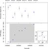 |
Fig. A.1 Fractional polarization (top) and EVPA (bottom) of the TeV source J0136+3905. Black circles are RoboPol data and blue triangles NOT data. The shaded region shows the period of a significant EVPA rotation. The inset in the lower panel shows the Q/I vs. U/I. EVPA data are shown only for observations where the signal to noise in the polarization fraction ≥3. |
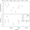 |
Fig. A.2 Fractional polarization (top) and EVPA (bottom) of the TeV source J0152+0146. Black circles are RoboPol data and blue triangles NOT data. The inset in the lower panel shows the Q/I vs. U/I. EVPA data are shown only for observations where the signal to noise in the polarization fraction ≥3. |
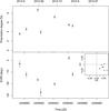 |
Fig. A.3 Fractional polarization (top) and EVPA (bottom) of the TeV source J0222+4302. The inset in the lower panel shows Q/I vs. U/I. EVPA data are shown only for observations where the signal to noise in the polarization fraction ≥3. |
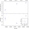 |
Fig. A.4 Fractional polarization (top) and EVPA (bottom) of the TeV source J0232+2017. The inset in the lower panel shows Q/I vs. U/I. EVPA data are shown only for observations where the signal to noise in the polarization fraction ≥3. |
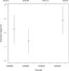 |
Fig. A.5 Fractional polarization (top) and EVPA (bottom) of the TeV source J0319+1845. None of the observations have polarization fraction ≥3 and no EVPA data are shown. |
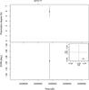 |
Fig. A.6 Fractional polarization (top) and EVPA (bottom) of the TeV source J0416+0105. The inset in the lower panel shows Q/I vs. U/I. EVPA data are shown only for observations where the signal to noise in the polarization fraction ≥3. |
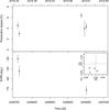 |
Fig. A.7 Fractional polarization (top) and EVPA (bottom) of the TeV source J0507+6737. The inset in the lower panel shows Q/I vs. U/I. EVPA data are shown only for observations where the signal to noise in the polarization fraction ≥3. |
 |
Fig. A.8 Fractional polarization (top) and EVPA (bottom) of the TeV source J0521+2112. The inset in the lower panel shows Q/I vs. U/I. EVPA data are shown only for observations where the signal to noise in the polarization fraction ≥3. |
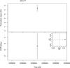 |
Fig. A.9 Fractional polarization (top) and EVPA (bottom) of the TeV source J0648+1516. The inset in the lower panel shows Q/I vs. U/I. EVPA data are shown only for observations where the signal to noise in the polarization fraction ≥3. |
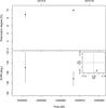 |
Fig. A.10 Fractional polarization (top) and EVPA (bottom) of the TeV source J0650+2502. The inset in the lower panel shows Q/I vs. U/I. EVPA data are shown only for observations where the signal to noise in the polarization fraction ≥3. |
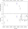 |
Fig. A.11 Fractional polarization (top) and EVPA (bottom) of the TeV source J0710+5908. The inset in the lower panel shows Q/I vs. U/I. EVPA data are shown only for observations where the signal to noise in the polarization fraction ≥3. |
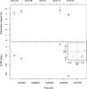 |
Fig. A.12 Fractional polarization (top) and EVPA (bottom) of the TeV source J0809+5218. The inset in the lower panel shows Q/I vs. U/I. EVPA data are shown only for observations where the signal to noise in the polarization fraction ≥3. |
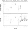 |
Fig. A.13 Fractional polarization (top) and EVPA (bottom) of the TeV source J1136+7009. The inset in the lower panel shows Q/I vs. U/I. EVPA data are shown only for observations where the signal to noise in the polarization fraction ≥3. |
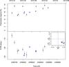 |
Fig. A.14 Fractional polarization (top) and EVPA (bottom) of the TeV source J1217+3007. Black circles are RoboPol data and blue triangles NOT data. The inset in the lower panel shows Q/I vs. U/I. EVPA data are shown only for observations where the signal to noise in the polarization fraction ≥3. |
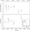 |
Fig. A.15 Fractional polarization (top) and EVPA (bottom) of the TeV source J1221+3010. Black circles are RoboPol data and blue triangles NOT data. The inset in the lower panel shows Q/I vs. U/I. EVPA data are shown only for observations where the signal to noise in the polarization fraction ≥3. |
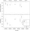 |
Fig. A.16 Fractional polarization (top) and EVPA (bottom) of the TeV source J1221+2813. The inset in the lower panel shows Q/I vs. U/I. EVPA data are shown only for observations where the signal to noise in the polarization fraction ≥3. |
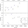 |
Fig. A.17 Fractional polarization (top) and EVPA (bottom) of the TeV source J1224+2436. Black circles are RoboPol data and blue triangles NOT data. The inset in the lower panel shows Q/I vs. U/I. EVPA data are shown only for observations where the signal to noise in the polarization fraction ≥3. |
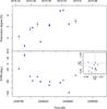 |
Fig. A.18 Fractional polarization (top) and EVPA (bottom) of the TeV source J1427+2348. Black circles are RoboPol data and blue triangles NOT data. The inset in the lower panel shows Q/I vs. U/I. EVPA data are shown only for observations where the signal to noise in the polarization fraction ≥3. |
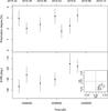 |
Fig. A.19 Fractional polarization (top) and EVPA (bottom) of the TeV source J1428+4240. The inset in the lower panel shows Q/I vs. U/I. EVPA data are shown only for observations where the signal to noise in the polarization fraction ≥3. |
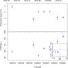 |
Fig. A.20 Fractional polarization (top) and EVPA (bottom) of the TeV source J1442+1200. The inset in the lower panel shows Q/I vs. U/I. EVPA data are shown only for observations where the signal to noise in the polarization fraction ≥3. |
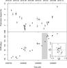 |
Fig. A.21 Fractional polarization (top) and EVPA (bottom) of the TeV source J1555+1111. The shaded region shows the period of a significant EVPA rotation. The inset in the lower panel shows Q/I vs. U/I. EVPA data are shown only for observations where the signal to noise in the polarization fraction ≥3. |
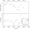 |
Fig. A.22 Fractional polarization (top) and EVPA (bottom) of the TeV source J1725+1152. The inset in the lower panel shows Q/I vs. U/I. EVPA data are shown only for observations where the signal to noise in the polarization fraction ≥3. |
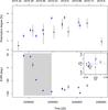 |
Fig. A.23 Fractional polarization (top) and EVPA (bottom) of the TeV source J1728+5013. Black circles are RoboPol data and blue triangles NOT data. The shaded region shows the period of a significant EVPA rotation. The inset in the lower panel shows Q/I vs. U/I. EVPA data are shown only for observations where the signal to noise in the polarization fraction ≥3. |
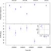 |
Fig. A.24 Fractional polarization (top) and EVPA (bottom) of the TeV source J1743+1935. The inset in the lower panel shows Q/I vs. U/I. EVPA data are shown only for observations where the signal to noise in the polarization fraction ≥3. |
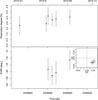 |
Fig. A.25 Fractional polarization (top) and EVPA (bottom) of the TeV source J1943+2118. The inset in the lower panel shows Q/I vs. U/I. EVPA data are shown only for observations where the signal to noise in the polarization fraction ≥3. |
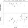 |
Fig. A.26 Fractional polarization (top) and EVPA (bottom) of the TeV source J1959+6508. The inset in the lower panel shows Q/I vs. U/I. EVPA data are shown only for observations where the signal to noise in the polarization fraction ≥3. |
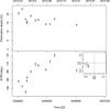 |
Fig. A.27 Fractional polarization (top) and EVPA (bottom) of the TeV source J2001+4352. The inset in the lower panel shows Q/I vs. U/I. EVPA data are shown only for observations where the signal to noise in the polarization fraction ≥3. |
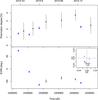 |
Fig. A.28 Fractional polarization (top) and EVPA (bottom) of the TeV source "J2250+3825. Black circles are RoboPol data and blue triangles NOT data. The inset in the lower panel shows Q/I vs. U/I. EVPA data are shown only for observations where the signal to noise in the polarization fraction ≥3. |
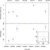 |
Fig. A.29 Fractional polarization (top) and EVPA (bottom) of the TeV source J2347+5142. The inset in the lower panel shows Q/I vs. U/I. EVPA data are shown only for observations where the signal to noise in the polarization fraction ≥3. |
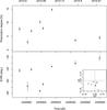 |
Fig. A.30 Fractional polarization (top) and EVPA (bottom) of the non-TeV source J0114+1325. The inset in the lower panel shows the Q/I vs. U/I from the RoboPol data. EVPA data are shown only for observations where the signal to noise in the polarization fraction ≥3. |
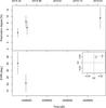 |
Fig. A.31 Fractional polarization (top) and EVPA (bottom) of the non-TeV source J0848+6606. The inset in the lower panel shows the Q/I vs. U/I from the RoboPol data. EVPA data are shown only for observations where the signal to noise in the polarization fraction ≥3. |
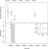 |
Fig. A.32 Fractional polarization (top) and EVPA (bottom) of the non-TeV source J1037+5711. The shaded region shows the period of a significant EVPA rotation. The inset in the lower panel shows the Q/I vs. U/I from the RoboPol data. EVPA data are shown only for observations where the signal to noise in the polarization fraction ≥3. |
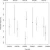 |
Fig. A.33 Fractional polarization (top) and EVPA (bottom) of the non-TeV source J1203+6031. None of the polarization observations have signal to noise ≥3 and no EVPA data are shown. |
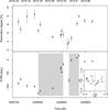 |
Fig. A.34 Fractional polarization (top) and EVPA (bottom) of the non-TeV source J1542+6129. The shaded region shows the period of a significant EVPA rotation. The inset in the lower panel shows the Q/I vs. U/I from the RoboPol data. EVPA data are shown only for observations where the signal to noise in the polarization fraction ≥3. |
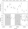 |
Fig. A.35 Fractional polarization (top) and EVPA (bottom) of the non-TeV source J1558+5625. The shaded region shows the period of a significant EVPA rotation. The inset in the lower panel shows the Q/I vs. U/I from the RoboPol data. EVPA data are shown only for observations where the signal to noise in the polarization fraction ≥3. |
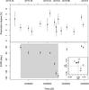 |
Fig. A.36 Fractional polarization (top) and EVPA (bottom) of the non-TeV source J1649+5235. The shaded region shows the period of a significant EVPA rotation. The inset in the lower panel shows the Q/I vs. U/I from the RoboPol data. EVPA data are shown only for observations where the signal to noise in the polarization fraction ≥3. |
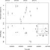 |
Fig. A.37 Fractional polarization (top) and EVPA (bottom) of the non-TeV source J1754+3212. The inset in the lower panel shows the Q/I vs. U/I from the RoboPol data. EVPA data are shown only for observations where the signal to noise in the polarization fraction ≥3. |
 |
Fig. A.38 Fractional polarization (top) and EVPA (bottom) of the non-TeV source J1809+2041. The shaded region shows the period of a significant EVPA rotation. The inset in the lower panel shows the Q/I vs. U/I from the RoboPol data. EVPA data are shown only for observations where the signal to noise in the polarization fraction ≥3. |
 |
Fig. A.39 Fractional polarization (top) and EVPA (bottom) of the non-TeV source J1813+3144. The inset in the lower panel shows the Q/I vs. U/I from the RoboPol data. EVPA data are shown only for observations where the signal to noise in the polarization fraction ≥3. |
 |
Fig. A.40 Fractional polarization (top) and EVPA (bottom) of the non-TeV source J1836+3136. The inset in the lower panel shows the Q/I vs. U/I from the RoboPol data. EVPA data are shown only for observations where the signal to noise in the polarization fraction ≥3. |
 |
Fig. A.41 Fractional polarization (top) and EVPA (bottom) of the non-TeV source J1838+4802. The inset in the lower panel shows the Q/I vs. U/I from the RoboPol data. EVPA data are shown only for observations where the signal to noise in the polarization fraction ≥3. |
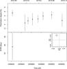 |
Fig. A.42 Fractional polarization (top) and EVPA (bottom) of the non-TeV source J1841+3218. The inset in the lower panel shows the Q/I vs. U/I from the RoboPol data. EVPA data are shown only for observations where the signal to noise in the polarization fraction ≥3. |
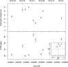 |
Fig. A.43 Fractional polarization (top) and EVPA (bottom) of the non-TeV source J1903+5540. The inset in the lower panel shows the Q/I vs. U/I from the RoboPol data. EVPA data are shown only for observations where the signal to noise in the polarization fraction ≥3. |
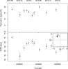 |
Fig. A.44 Fractional polarization (top) and EVPA (bottom) of the non-TeV source J2015-0137. The inset in the lower panel shows the Q/I vs. U/I from the RoboPol data. EVPA data are shown only for observations where the signal to noise in the polarization fraction ≥3. |
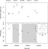 |
Fig. A.45 Fractional polarization (top) and EVPA (bottom) of the non-TeV source J2022+7611. The shaded region shows the period of a significant EVPA rotation. The inset in the lower panel shows the Q/I vs. U/I from the RoboPol data. EVPA data are shown only for observations where the signal to noise in the polarization fraction ≥3. |
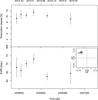 |
Fig. A.46 Fractional polarization (top) and EVPA (bottom) of the non-TeV source J2131-0915. The inset in the lower panel shows the Q/I vs. U/I from the RoboPol data. EVPA data are shown only for observations where the signal to noise in the polarization fraction ≥3. |
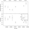 |
Fig. A.47 Fractional polarization (top) and EVPA (bottom) of the non-TeV source J2149+0322. The inset in the lower panel shows the Q/I vs. U/I from the RoboPol data. EVPA data are shown only for observations where the signal to noise in the polarization fraction ≥3. |
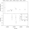 |
Fig. A.48 Fractional polarization (top) and EVPA (bottom) of the non-TeV source J2340+8015. The inset in the lower panel shows the Q/I vs. U/I from the RoboPol data. EVPA data are shown only for observations where the signal to noise in the polarization fraction ≥3. |
All Tables
All Figures
|
Fig. 1 Stacked histogram of the redshift in the TeV (white) and non-TeV (gray) samples. The hatched bars show the fraction of sources with lower limit redshifts. |
| In the text | |
|
Fig. 2 Top: stacked histogram of the intrinsic mean polarization fraction in the TeV (white) and non-TeV (gray) samples. Bottom: stacked histogram of the intrinsic modulation index in the TeV (white) and non-TeV (gray) samples. The hatched bars show the fraction of TeV or non-TeV sources that have only 2σ upper limits available. |
| In the text | |
|
Fig. 3 Top: stacked histogram of the extinction-corrected mean magnitude in the TeV (white) and non-TeV (gray) samples. Bottom: stacked histogram of the host-corrected mean magnitude in the TeV (white hatched) and non-TeV (gray hatched) samples. For sources where a host correction is not available, we show the extinction-corrected mean magnitudes as in the top panel. |
| In the text | |
|
Fig. 4 Stacked histogram of the median EVPA derivative for the TeV (white) and non-TeV (gray) samples. Top panel: shows the distribution when the derivative is set to zero for insignificant changes and the bottom panel shows the same when insignificant changes are ignored (see text for details). |
| In the text | |
|
Fig. 5 Top: stacked histogram of the distance of the mass center in the Q/I−U/I plane from the origin. Bottom: stacked histogram of the mean distance of the Q/I vs. U/I points from the mass center. The TeV sources are shown in white and non-TeV sources in gray. |
| In the text | |
|
Fig. 6 Intrinsic modulation index against the intrinsic mean polarization fraction for the TeV (black circles) and non-TeV (red open squares) sources. Lower limits in modulation index are shown with downward triangles. |
| In the text | |
|
Fig. 7 Stacked histogram of the difference between the mean optical EVPA and inner jet position angle from VLBI observations for the TeV sources showing indications of a preferred polarization angle. |
| In the text | |
|
Fig. 8 Top: stacked Q/I vs. U/I plot for the TeV (left) and non-TeV (right) samples. Bottom: same for three TeV sources (left) and two non-TeV sources (right) for which we have data over multiple seasons. The stacking is performed by shifting the mass center of each source to the origin. In the bottom panel we stacked the data based on the mass center of all data, which is why the top and bottom panels are not exactly the same for the 2014 data. |
| In the text | |
|
Fig. 9 Frequency of rotations per 100 days for various combinations of the number of cells Ncells and number of them nvar that change during each step. |
| In the text | |
|
Fig. 10 Probability of observing n = 0,1,2 observations during our observing season for the TeV source RGB J0136+391 (top) and the non-TeV source GB6 J1037+5711 (bottom). The color scale shows the probability for a various set of parameters nvar and Ncells. The white dot indicates the best-fit region for obtaining a similar polarization fraction as in the observed light curve and the black curves show its 95% confidence interval. |
| In the text | |
|
Fig. A.1 Fractional polarization (top) and EVPA (bottom) of the TeV source J0136+3905. Black circles are RoboPol data and blue triangles NOT data. The shaded region shows the period of a significant EVPA rotation. The inset in the lower panel shows the Q/I vs. U/I. EVPA data are shown only for observations where the signal to noise in the polarization fraction ≥3. |
| In the text | |
|
Fig. A.2 Fractional polarization (top) and EVPA (bottom) of the TeV source J0152+0146. Black circles are RoboPol data and blue triangles NOT data. The inset in the lower panel shows the Q/I vs. U/I. EVPA data are shown only for observations where the signal to noise in the polarization fraction ≥3. |
| In the text | |
|
Fig. A.3 Fractional polarization (top) and EVPA (bottom) of the TeV source J0222+4302. The inset in the lower panel shows Q/I vs. U/I. EVPA data are shown only for observations where the signal to noise in the polarization fraction ≥3. |
| In the text | |
|
Fig. A.4 Fractional polarization (top) and EVPA (bottom) of the TeV source J0232+2017. The inset in the lower panel shows Q/I vs. U/I. EVPA data are shown only for observations where the signal to noise in the polarization fraction ≥3. |
| In the text | |
|
Fig. A.5 Fractional polarization (top) and EVPA (bottom) of the TeV source J0319+1845. None of the observations have polarization fraction ≥3 and no EVPA data are shown. |
| In the text | |
|
Fig. A.6 Fractional polarization (top) and EVPA (bottom) of the TeV source J0416+0105. The inset in the lower panel shows Q/I vs. U/I. EVPA data are shown only for observations where the signal to noise in the polarization fraction ≥3. |
| In the text | |
|
Fig. A.7 Fractional polarization (top) and EVPA (bottom) of the TeV source J0507+6737. The inset in the lower panel shows Q/I vs. U/I. EVPA data are shown only for observations where the signal to noise in the polarization fraction ≥3. |
| In the text | |
|
Fig. A.8 Fractional polarization (top) and EVPA (bottom) of the TeV source J0521+2112. The inset in the lower panel shows Q/I vs. U/I. EVPA data are shown only for observations where the signal to noise in the polarization fraction ≥3. |
| In the text | |
|
Fig. A.9 Fractional polarization (top) and EVPA (bottom) of the TeV source J0648+1516. The inset in the lower panel shows Q/I vs. U/I. EVPA data are shown only for observations where the signal to noise in the polarization fraction ≥3. |
| In the text | |
|
Fig. A.10 Fractional polarization (top) and EVPA (bottom) of the TeV source J0650+2502. The inset in the lower panel shows Q/I vs. U/I. EVPA data are shown only for observations where the signal to noise in the polarization fraction ≥3. |
| In the text | |
|
Fig. A.11 Fractional polarization (top) and EVPA (bottom) of the TeV source J0710+5908. The inset in the lower panel shows Q/I vs. U/I. EVPA data are shown only for observations where the signal to noise in the polarization fraction ≥3. |
| In the text | |
|
Fig. A.12 Fractional polarization (top) and EVPA (bottom) of the TeV source J0809+5218. The inset in the lower panel shows Q/I vs. U/I. EVPA data are shown only for observations where the signal to noise in the polarization fraction ≥3. |
| In the text | |
|
Fig. A.13 Fractional polarization (top) and EVPA (bottom) of the TeV source J1136+7009. The inset in the lower panel shows Q/I vs. U/I. EVPA data are shown only for observations where the signal to noise in the polarization fraction ≥3. |
| In the text | |
|
Fig. A.14 Fractional polarization (top) and EVPA (bottom) of the TeV source J1217+3007. Black circles are RoboPol data and blue triangles NOT data. The inset in the lower panel shows Q/I vs. U/I. EVPA data are shown only for observations where the signal to noise in the polarization fraction ≥3. |
| In the text | |
|
Fig. A.15 Fractional polarization (top) and EVPA (bottom) of the TeV source J1221+3010. Black circles are RoboPol data and blue triangles NOT data. The inset in the lower panel shows Q/I vs. U/I. EVPA data are shown only for observations where the signal to noise in the polarization fraction ≥3. |
| In the text | |
|
Fig. A.16 Fractional polarization (top) and EVPA (bottom) of the TeV source J1221+2813. The inset in the lower panel shows Q/I vs. U/I. EVPA data are shown only for observations where the signal to noise in the polarization fraction ≥3. |
| In the text | |
|
Fig. A.17 Fractional polarization (top) and EVPA (bottom) of the TeV source J1224+2436. Black circles are RoboPol data and blue triangles NOT data. The inset in the lower panel shows Q/I vs. U/I. EVPA data are shown only for observations where the signal to noise in the polarization fraction ≥3. |
| In the text | |
|
Fig. A.18 Fractional polarization (top) and EVPA (bottom) of the TeV source J1427+2348. Black circles are RoboPol data and blue triangles NOT data. The inset in the lower panel shows Q/I vs. U/I. EVPA data are shown only for observations where the signal to noise in the polarization fraction ≥3. |
| In the text | |
|
Fig. A.19 Fractional polarization (top) and EVPA (bottom) of the TeV source J1428+4240. The inset in the lower panel shows Q/I vs. U/I. EVPA data are shown only for observations where the signal to noise in the polarization fraction ≥3. |
| In the text | |
|
Fig. A.20 Fractional polarization (top) and EVPA (bottom) of the TeV source J1442+1200. The inset in the lower panel shows Q/I vs. U/I. EVPA data are shown only for observations where the signal to noise in the polarization fraction ≥3. |
| In the text | |
|
Fig. A.21 Fractional polarization (top) and EVPA (bottom) of the TeV source J1555+1111. The shaded region shows the period of a significant EVPA rotation. The inset in the lower panel shows Q/I vs. U/I. EVPA data are shown only for observations where the signal to noise in the polarization fraction ≥3. |
| In the text | |
|
Fig. A.22 Fractional polarization (top) and EVPA (bottom) of the TeV source J1725+1152. The inset in the lower panel shows Q/I vs. U/I. EVPA data are shown only for observations where the signal to noise in the polarization fraction ≥3. |
| In the text | |
|
Fig. A.23 Fractional polarization (top) and EVPA (bottom) of the TeV source J1728+5013. Black circles are RoboPol data and blue triangles NOT data. The shaded region shows the period of a significant EVPA rotation. The inset in the lower panel shows Q/I vs. U/I. EVPA data are shown only for observations where the signal to noise in the polarization fraction ≥3. |
| In the text | |
|
Fig. A.24 Fractional polarization (top) and EVPA (bottom) of the TeV source J1743+1935. The inset in the lower panel shows Q/I vs. U/I. EVPA data are shown only for observations where the signal to noise in the polarization fraction ≥3. |
| In the text | |
|
Fig. A.25 Fractional polarization (top) and EVPA (bottom) of the TeV source J1943+2118. The inset in the lower panel shows Q/I vs. U/I. EVPA data are shown only for observations where the signal to noise in the polarization fraction ≥3. |
| In the text | |
|
Fig. A.26 Fractional polarization (top) and EVPA (bottom) of the TeV source J1959+6508. The inset in the lower panel shows Q/I vs. U/I. EVPA data are shown only for observations where the signal to noise in the polarization fraction ≥3. |
| In the text | |
|
Fig. A.27 Fractional polarization (top) and EVPA (bottom) of the TeV source J2001+4352. The inset in the lower panel shows Q/I vs. U/I. EVPA data are shown only for observations where the signal to noise in the polarization fraction ≥3. |
| In the text | |
|
Fig. A.28 Fractional polarization (top) and EVPA (bottom) of the TeV source "J2250+3825. Black circles are RoboPol data and blue triangles NOT data. The inset in the lower panel shows Q/I vs. U/I. EVPA data are shown only for observations where the signal to noise in the polarization fraction ≥3. |
| In the text | |
|
Fig. A.29 Fractional polarization (top) and EVPA (bottom) of the TeV source J2347+5142. The inset in the lower panel shows Q/I vs. U/I. EVPA data are shown only for observations where the signal to noise in the polarization fraction ≥3. |
| In the text | |
|
Fig. A.30 Fractional polarization (top) and EVPA (bottom) of the non-TeV source J0114+1325. The inset in the lower panel shows the Q/I vs. U/I from the RoboPol data. EVPA data are shown only for observations where the signal to noise in the polarization fraction ≥3. |
| In the text | |
|
Fig. A.31 Fractional polarization (top) and EVPA (bottom) of the non-TeV source J0848+6606. The inset in the lower panel shows the Q/I vs. U/I from the RoboPol data. EVPA data are shown only for observations where the signal to noise in the polarization fraction ≥3. |
| In the text | |
|
Fig. A.32 Fractional polarization (top) and EVPA (bottom) of the non-TeV source J1037+5711. The shaded region shows the period of a significant EVPA rotation. The inset in the lower panel shows the Q/I vs. U/I from the RoboPol data. EVPA data are shown only for observations where the signal to noise in the polarization fraction ≥3. |
| In the text | |
|
Fig. A.33 Fractional polarization (top) and EVPA (bottom) of the non-TeV source J1203+6031. None of the polarization observations have signal to noise ≥3 and no EVPA data are shown. |
| In the text | |
|
Fig. A.34 Fractional polarization (top) and EVPA (bottom) of the non-TeV source J1542+6129. The shaded region shows the period of a significant EVPA rotation. The inset in the lower panel shows the Q/I vs. U/I from the RoboPol data. EVPA data are shown only for observations where the signal to noise in the polarization fraction ≥3. |
| In the text | |
|
Fig. A.35 Fractional polarization (top) and EVPA (bottom) of the non-TeV source J1558+5625. The shaded region shows the period of a significant EVPA rotation. The inset in the lower panel shows the Q/I vs. U/I from the RoboPol data. EVPA data are shown only for observations where the signal to noise in the polarization fraction ≥3. |
| In the text | |
|
Fig. A.36 Fractional polarization (top) and EVPA (bottom) of the non-TeV source J1649+5235. The shaded region shows the period of a significant EVPA rotation. The inset in the lower panel shows the Q/I vs. U/I from the RoboPol data. EVPA data are shown only for observations where the signal to noise in the polarization fraction ≥3. |
| In the text | |
|
Fig. A.37 Fractional polarization (top) and EVPA (bottom) of the non-TeV source J1754+3212. The inset in the lower panel shows the Q/I vs. U/I from the RoboPol data. EVPA data are shown only for observations where the signal to noise in the polarization fraction ≥3. |
| In the text | |
|
Fig. A.38 Fractional polarization (top) and EVPA (bottom) of the non-TeV source J1809+2041. The shaded region shows the period of a significant EVPA rotation. The inset in the lower panel shows the Q/I vs. U/I from the RoboPol data. EVPA data are shown only for observations where the signal to noise in the polarization fraction ≥3. |
| In the text | |
|
Fig. A.39 Fractional polarization (top) and EVPA (bottom) of the non-TeV source J1813+3144. The inset in the lower panel shows the Q/I vs. U/I from the RoboPol data. EVPA data are shown only for observations where the signal to noise in the polarization fraction ≥3. |
| In the text | |
|
Fig. A.40 Fractional polarization (top) and EVPA (bottom) of the non-TeV source J1836+3136. The inset in the lower panel shows the Q/I vs. U/I from the RoboPol data. EVPA data are shown only for observations where the signal to noise in the polarization fraction ≥3. |
| In the text | |
|
Fig. A.41 Fractional polarization (top) and EVPA (bottom) of the non-TeV source J1838+4802. The inset in the lower panel shows the Q/I vs. U/I from the RoboPol data. EVPA data are shown only for observations where the signal to noise in the polarization fraction ≥3. |
| In the text | |
|
Fig. A.42 Fractional polarization (top) and EVPA (bottom) of the non-TeV source J1841+3218. The inset in the lower panel shows the Q/I vs. U/I from the RoboPol data. EVPA data are shown only for observations where the signal to noise in the polarization fraction ≥3. |
| In the text | |
|
Fig. A.43 Fractional polarization (top) and EVPA (bottom) of the non-TeV source J1903+5540. The inset in the lower panel shows the Q/I vs. U/I from the RoboPol data. EVPA data are shown only for observations where the signal to noise in the polarization fraction ≥3. |
| In the text | |
|
Fig. A.44 Fractional polarization (top) and EVPA (bottom) of the non-TeV source J2015-0137. The inset in the lower panel shows the Q/I vs. U/I from the RoboPol data. EVPA data are shown only for observations where the signal to noise in the polarization fraction ≥3. |
| In the text | |
|
Fig. A.45 Fractional polarization (top) and EVPA (bottom) of the non-TeV source J2022+7611. The shaded region shows the period of a significant EVPA rotation. The inset in the lower panel shows the Q/I vs. U/I from the RoboPol data. EVPA data are shown only for observations where the signal to noise in the polarization fraction ≥3. |
| In the text | |
|
Fig. A.46 Fractional polarization (top) and EVPA (bottom) of the non-TeV source J2131-0915. The inset in the lower panel shows the Q/I vs. U/I from the RoboPol data. EVPA data are shown only for observations where the signal to noise in the polarization fraction ≥3. |
| In the text | |
|
Fig. A.47 Fractional polarization (top) and EVPA (bottom) of the non-TeV source J2149+0322. The inset in the lower panel shows the Q/I vs. U/I from the RoboPol data. EVPA data are shown only for observations where the signal to noise in the polarization fraction ≥3. |
| In the text | |
|
Fig. A.48 Fractional polarization (top) and EVPA (bottom) of the non-TeV source J2340+8015. The inset in the lower panel shows the Q/I vs. U/I from the RoboPol data. EVPA data are shown only for observations where the signal to noise in the polarization fraction ≥3. |
| In the text | |
Current usage metrics show cumulative count of Article Views (full-text article views including HTML views, PDF and ePub downloads, according to the available data) and Abstracts Views on Vision4Press platform.
Data correspond to usage on the plateform after 2015. The current usage metrics is available 48-96 hours after online publication and is updated daily on week days.
Initial download of the metrics may take a while.