| Issue |
A&A
Volume 596, December 2016
|
|
|---|---|---|
| Article Number | A74 | |
| Number of page(s) | 15 | |
| Section | Planets and planetary systems | |
| DOI | https://doi.org/10.1051/0004-6361/201628955 | |
| Published online | 02 December 2016 | |
Evolution of protoplanetary discs with magnetically driven disc winds
1 School of Arts & Sciences, University of Tokyo, 3-8-1, Komaba, Meguro, 153-8902 Tokyo, Japan
e-mail: stakeru@ea.c.u-tokyo.ac.jp
2 Department of Physics, Nagoya University, Nagoya, 464-8602 Aichi, Japan
3 Laboratoire Lagrange, Université Côte d’Azur, Observatoire de la Côte d’Azur, CNRS, Boulevard de l’Observatoire, CS 34229, 06304 Nice Cedex 4, France
4 Division of Theoretical Astronomy, National Astronomical Observatory of Japan, 2-21-1, Osawa, Mitaka, 181-8588 Tokyo, Japan
5 Institut Universitaire de France, 103 boulevard Saint-Michel, 75005 Paris, France
Received: 18 May 2016
Accepted: 1 September 2016
Aims. We investigate the evolution of protoplanetary discs (PPDs) with magnetically driven disc winds and viscous heating.
Methods. We considered an initially massive disc with ~0.1 M⊙ to track the evolution from the early stage of PPDs. We solved the time evolution of surface density and temperature by taking into account viscous heating and the loss of mass and angular momentum by the disc winds within the framework of a standard α model for accretion discs. Our model parameters, turbulent viscosity, disc wind mass-loss, and disc wind torque, which were adopted from local magnetohydrodynamical simulations and constrained by the global energetics of the gravitational accretion, largely depends on the physical condition of PPDs, particularly on the evolution of the vertical magnetic flux in weakly ionized PPDs.
Results. Although there are still uncertainties concerning the evolution of the vertical magnetic flux that remains, the surface densities show a large variety, depending on the combination of these three parameters, some of which are very different from the surface density expected from the standard accretion. When a PPD is in a wind-driven accretion state with the preserved vertical magnetic field, the radial dependence of the surface density can be positive in the inner region <1−10 au. The mass accretion rates are consistent with observations, even in the very low level of magnetohydrodynamical turbulence. Such a positive radial slope of the surface density strongly affects planet formation because it inhibits the inward drift or even causes the outward drift of pebble- to boulder-sized solid bodies, and it also slows down or even reversed the inward type-I migration of protoplanets.
Conclusions. The variety of our calculated PPDs should yield a wide variety of exoplanet systems.
Key words: accretion, accretion disks / ISM: jets and outflows / magnetohydrodynamics (MHD) / protoplanetary disks / stars: winds, outflows / turbulence
© ESO, 2016
1. Introduction
The evolution of protoplanetary disks (PPDs) is one of the keys to understand planet formation. There are still several unsolved problems, one of which is the dispersal of PPDs (Haisch et al. 2001; Hernández et al. 2008; Takagi et al. 2014, 2015). The evolution and dispersal of PPDs have been extensively studied in the framework of viscously accreting discs that undergo photoevaporation by the irradiation from the central star (e.g., Shu et al. 1993; Hollenbach et al. 2000; Alexander et al. 2006; Kimura et al. 2016).
In addition to the viscous accretion and the photoevaporation, the role of magnetically driven disc winds has recently been received new attention. Suzuki & Inutsuka (2009) and Suzuki et al. (2010) proposed that vertical outflows driven by magnetohydrodynamical (MHD) turbulence might be a viable mechanism that disperses the gas component of PPDs; turbulence is triggered by magnetorotational instability (MRI; Velikhov 1959; Chandrasekhar 1961; Balbus & Hawley 1991), and the Poynting flux associated with the MHD turbulence drives vertical outflows. The idea of MHD turbulence-driven outflow has also been extended by considering various effects, such as a stronger magnetic field (Bai & Stone 2013a), a large-scale magnetic field (Lesur et al. 2013), and the dynamics of dust grains (Miyake et al. 2016), whereas its mass flux is still quantitatively uncertain (Fromang et al. 2013).
Although Suzuki et al. (2010) considered mass loss to be the sole role of the disc wind, the disc wind in reality also carries off the angular momentum (Blandford & Payne 1982; Pelletier & Pudritz 1992; Ferreira et al. 2006; Salmeron et al. 2011). In particular, a dead zone, which is an MRI-inactive region because of the insufficient ionization, is supposed to form in a PPD (Gammie 1996; Sano et al. 2000). In a dead zone the level of the excited turbulence is low, and it is not sufficient to sustain the observed mass accretion onto the central star. In these circumstances, the extraction of the angular momentum by the disc wind possibly plays a primary role in driving mass accretion (Bai & Stone 2013b; Simon et al. 2013). Bai et al. (2016) and Bai (2016) investigated the global evolution of PPDs in such a wind-driven accretion state, by also taking the effect of external heating into account, and reported that a large portion of the mass is removed by the disc wind in comparison to the accreting mass.
A critical open question concerning the disc wind from PPDs is that the mass-loss rate. At the later stage of the evolution, a wind footpoint that is determined by the irradiation from a central star is expected to primarily control the mass-loss rate (Bai et al. 2016; Bai 2016). On the other hand, at the earlier stage when the surface density is high, viscous heating plays an essential role in determining the thermal properties of PPDs (e.g., Ruden & Lin 1986; Nakamoto & Nakagawa 1994; Hirose & Turner 2011; Oka et al. 2011; Bitsch et al. 2015). To investigate the time evolution from the early epoch, we here take the effect of viscous heating in the global evolution of PPDs into account in addition to the loss of mass and angular momentum by the disc wind. We focus in particular on the conditions that create a density structure that is very different from the structure of classic viscously accreting discs, which may help solving long-standing problems such as the radial migration of pebbles, boulders, and protoplanets. For this goal, we evaluate the mass-loss rate from the global energetics of PPDs; the kinetic energy of the vertical outflow is mainly supplied from the gravitational accretion energy. This strategy is different from the method adopted by Bai (2016), in which the mass-loss rate was estimated based on the local profile of magnetically driven wind with external heating. A comparison between the two models is provided in Sect. 4.4.
2. Model
2.1. Basic definitions
We investigated the time evolution of PPDs with magnetically driven disc winds. Suzuki et al. (2010) solved the evolution of PPDs with MRI-triggered disc winds under simplified assumptions: the temperature is locally constant with time, and the disc wind only contributes to the mass loss without removing additional angular momentum. In this paper, we relaxed these assumptions to treat more realistic evolution of PPDs. We considered the heating by viscous accretion (Shakura & Sunyaev 1973; Nakamoto & Nakagawa 1994; Hueso & Guillot 2005) and the effect of disc wind torque on mass accretion (Blandford & Payne 1982; Pelletier & Pudritz 1992; Salmeron et al. 2011; Bai & Stone 2013b)
Throughout this paper, we assume that each annulus at radial distance r from a central star almost rotates with Keplerian frequency, ΩK (1)where G is the gravitational constant and M⋆ is the mass of the central star. We considered a central star with solar mass, M⋆ = M⊙. We defined a vertical scale height, H, of a disc
  (2)where cs is the sound speed. Temperature T and cs are related through
  (3)where kB is the Boltzmann constant, mH is the proton mass, and we assume mean molecular weight, μ = 2.34 (Hayashi 1981). A different definition for the scale height from ours, cs/ Ω (without
  ), is sometimes used in literatures.
2.2. Evolution of surface density
We treated the time evolution of the radial profile of surface density, Σ = ∫dzρ, of a disc (1 + 1 D model), while basic formula transformation is done in cylindrical coordinates, (r,φ,z). The time evolution of Σ(r) can be expressed as (see Appendix A for the derivation)
![\begin{eqnarray} &&\frac{\partial \Sigma}{\partial t} - \frac{1}{r}\frac{\partial}{\partial r} \left[\frac{2}{r\Omega}\left\{\frac{\partial}{\partial r}\left(r^2 \int {\rm d}z \left(\rho v_r \delta v_{\phi} - \frac{B_rB_{\phi}}{4\pi}\right)\right) \right.\right. \nonumber\\ && \left.\left. \qquad\qquad + r^2 \left(\rho \delta v_{\phi} v_z - \frac{B_{\phi}B_z}{4\pi}\right)_{\rm w} \right\}\right] + (\rho v_z)_{\rm w} = 0, \label{eq:sgmevlori} \end{eqnarray}](/articles/aa/full_html/2016/12/aa28955-16/aa28955-16-eq26.png)
where δvφ = vφ−rΩ is the deviation from the background rotation, and the subscript w stands for disc wind (see below). The [···] parenthesis of the second term represents radial mass flow,
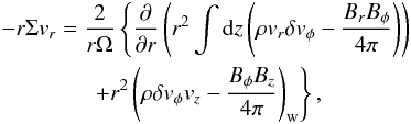
which is derived from the radial balance of angular momentum (Appendix A), and the third term of Eq. (4) denotes the mass loss by the disc wind. The second term consists of the rφ and φz components of Reynolds and Maxwell stresses. The rφ component represents the mass accretion (or decretion) induced by the transport of angular momentum through MHD turbulence. We used the following parametrization based on the α-prescription introduced by Shakura & Sunyaev (1973): 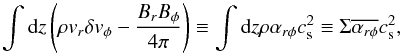 (6)where
  is the mass-weighted vertical average of αrφ. αrφ is a nondimensional parameter normalized by gas pressure (
 ) that describes the transport of angular momentum. We considered αrφ to originate from the MHD turbulence induced by MRI.
  depends on physical conditions of PPDs, such as the ionization and the strength of poloidal magnetic field; see Sect. 2.6 for our adopted values. Although we did not separate the contributions from the Reynolds stress (ρvrδvφ) and from the Maxwell stress (− BrBφ/ 4π> 0), the latter usually dominates the former by a factor of ~4 in accretion discs with MRI turbulence (Sano et al. 2004; Pessah et al. 2006; Hawley et al. 2011) .
is an effective turbulent viscosity, and it is mathematically related to viscosity, ν, appeared in a hydrodynamical equation, 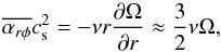 (7)where the second equality comes from the condition of the Keplerian rotation. The definition of α is not consistent throughout the literature; for example, ν ≈ αtHcs, is often used conventionally (e.g., Balbus & Hawley 1998). These two α’s are related by
  , where note again that the definition of H (Eq. (2)) is also not consistent in the literatures.
The φz component of the second term of Eq. (4) indicates the mass accretion induced by the angular momentum loss with magnetized disc winds, which was not taken into account in Suzuki et al. (2010). The term of (··· )w represents the sum of the angular momentum flux density carried away by the magnetized outflows from the top and bottom surfaces of a disc. While Reynolds (ρδvφvz) and Maxwell (− BφBz/ 4π( > 0)) stresses contribute to the φz stress as well, the latter usually dominates in magnetized accretion discs (e.g., Pelletier & Pudritz 1992), similarly to the rφ component. This magnetic braking effect needs to be evaluated in the wind region where it operates; this is the reason why the subscript w is necessary in this term. To incorporate the effect of the wind torque into the 1+1D (t–r) model, αφz needs to be evaluated by physical quantities at the midplane, and we adopted a similar parametrization to the rφ component,  (8)where we define the nondimensional stress,
  , normalized by density,
  , at the midplane,
The third term, (ρvz)w, of Eq. (4) represents the sum of the mass loss by the vertical outflows from the upper and lower disc surfaces. Suzuki et al. (2010) introduced the nondimensional mass flux normalized by the density and the sound speed at the midplane:  (9)We model Cw in Sect. 2.3.
Substituting Eqs. (6), (8), and (9) into Eq. (4), we finally have ![\begin{eqnarray} \frac{\partial \Sigma}{\partial t}& -& \frac{1}{r}\frac{\partial}{\partial r} \left[\frac{2}{r\Omega}\left\{\frac{\partial}{\partial r}(r^2 \Sigma \overline{\alpha_{r\phi}}c_{\rm s}^2) + r^2 \overline{\alpha_{\phi z}} (\rho c_{\rm s}^2)_{\rm mid} \right\}\right] \nonumber\\ &&\qquad\qquad \qquad \qquad\, \qquad+ C_{\rm w}(\rho c_{\rm s})_{\rm mid} = 0. \label{eq:sgmevl} \end{eqnarray}](/articles/aa/full_html/2016/12/aa28955-16/aa28955-16-eq56.png) (10)We solved this equation for different sets of the three parameters, , , and Cw. We note that Bai (2016) recently derived essentially the same equation in a different form using mass-loss rate and mass accretion rate instead of the above three-dimensionless parameters.
(10)We solved this equation for different sets of the three parameters, , , and Cw. We note that Bai (2016) recently derived essentially the same equation in a different form using mass-loss rate and mass accretion rate instead of the above three-dimensionless parameters.
2.3. Mass-loss rate by disc winds: energetics
We assumed that the energy of the disc wind originates from gravitational accretion. Then, the mass flux of the disc wind, Cw, is constrained by and . A starting point for this energetics constraint is the conservation equation of total MHD energy (e.g., Balbus & Hawley 1998),
![\begin{eqnarray} &&\frac{\partial}{\partial t}\left[\frac{1}{2}\rho v^2 + \rho \Phi +\frac{p}{\gamma -1} + \frac{B^2}{8\pi} \right] +\mbf{\nabla\cdot}\left[\mbf{v}\left(\frac{1}{2}\rho v^2 + \rho \Phi +\frac{\gamma p}{\gamma -1} \right) \right. \nonumber\\ &&\left. \qquad +\frac{\mbf{B}}{4\pi}\times (\mbf{v}\times\mbf{B}) + \mbf{F}_{\rm ot}\right] = 0, \label{eq:totengMHD} \end{eqnarray}](/articles/aa/full_html/2016/12/aa28955-16/aa28955-16-eq57.png)
where p is the gas pressure, γ is a ratio of specific heats,  is the gravitational potential by a central star, and Fot is other contributions to energy flux in addition to the MHD energy, such as thermal conduction and radiative heating or cooling. We considered thin discs with nearly Keplerian rotation (Eq. (1)), and hence, we can assume
  , and safely neglect the terms concerning gas pressure. Leaving dominant terms in Eq. (11) we finally obtained an approximated energy equation as (Appendix B; Eq. (B.8))
![\begin{eqnarray} \frac{\partial}{\partial t}\left(-\Sigma \frac{r^2\Omega^2}{2}\right) +\frac{1}{r}\frac{\partial}{\partial r}\left[r\Omega \left\{\frac{\partial}{\partial r}(r^2 \Sigma \overline{\alpha_{r\phi}}c_{\rm s}^2) + r^2 \overline{\alpha_{\phi z}} (\rho c_{\rm s}^2)_{\rm mid} \right\} \right. \nonumber\\ \left. + r^2\Omega\Sigma\overline{\alpha_{r \phi}} c_{\rm s}^2\right] + (\rho v_z)_{\rm w} E_{\rm w}+ F_{\rm rad} =0, \label{eq:totengring} \end{eqnarray}](/articles/aa/full_html/2016/12/aa28955-16/aa28955-16-eq63.png)
where Ew is the specific total energy of the gas in the disc wind; (ρvz)wEw is the energy carried away by the disc wind. Frad is radiation loss from the top and bottom surfaces,  (13)where σSB is the Stefan-Boltzmann constant and Tsurf is the temperature at the disc surfaces. We here neglected the energy gain by the irradiation from a central star (Kusaka et al. 1970; Dullemond et al. 2002; Davis 2005) and other external sources. The effect of stellar irradiation was taken into account later when we estimated the temperature.
Equation (12) contains two terms with ; the first term in {···} denotes the liberated gravitational energy by mass accretion, and second term outside {···} represents heating by turbulent dissipation, which phenomenologically corresponds to viscous heating. The wind torque, , does not contribute to this effective viscous heating because the disc wind does not transport angular momentum within the disc but simply removes it, although contributes to the mass accretion.
Using Eq. (10), we can eliminate the time derivative term of Eq. (12) to derive an energetics constraint on the disc wind (Appendix B):
![\begin{eqnarray} &&(\rho v_z)_{\rm w}\left(E_{\rm w}+\frac{r^2\Omega^2}{2}\right) + F_{\rm rad}=~~~~~~~~~~~~~~~~~~~~~~~~~~~~~~~~~~~~~~~~~~~~~~~~~~~~~~~~~~~ \nonumber\\ &&\,\,\,\,\,\, \frac{\Omega}{r}\left[\frac{\partial}{\partial r}(r^2 \Sigma \overline{\alpha_{r\phi}}c_{\rm s}^2) + r^2 \overline{\alpha_{\phi z}}(\rho c_{\rm s}^2)_{\rm mid}\right] -\frac{1}{r}\frac{\partial}{\partial r}\left(r^2 \Sigma\Omega \overline{\alpha_{r\phi}}c_{\rm s}^2\right) \label{eq:engcnt1} \\ &&\,\,\,\,\,\,=\frac{3}{2}\Omega\Sigma\overline{\alpha_{r\phi}}c_{\rm s}^2 + r\Omega \overline{\alpha_{\phi z}}(\rho c_{\rm s}^2)_{\rm mid} . \label{eq:engcnt2} \end{eqnarray}](/articles/aa/full_html/2016/12/aa28955-16/aa28955-16-eq71.png)
The physical meaning of Eq. (14) is that the energy carried away by disc winds (first term on the left-hand side; l.h.s. hereafter) and radiation (second term on the l.h.s.) is determined by the gravitational energy liberated by accretion (first term on the right-hand side; r.h.s. hereafter) and effective viscous heating (second term on the r.h.s.). We used the Keplerian rotation (Eq. (1)) to transform Eqs. (14) to (15). The term with includes contributions from the gravitational accretion and from the effective viscous heating.
Suzuki et al. (2010) assumed that  is the condition to drive the vertical outflow to a large distance (Eq. (22) of Suzuki et al. 2010). However, we adopt Ew ≥ 0, because this is the sufficient condition for the wind material to reach z ⇒ ∞ (
 in Eq. (B.5)). Following this consideration, we derived the mass flux of the disc wind that satisfies the energetics constraint with Ew = 0 from Eqs. (14) and (15) in a nondimensional form:
  where Cw,e stands for the mass flux constrained by the energetics. We here used
  , and for the last equality we introduced an aspect ratio,
  .
.
It is crucial to determine the fractions of the energy transferred to the disc winds (first term on the l.h.s. of Eq. (16)) and to the radiation loss (second term). Following the standard accretion disc model (Shakura & Sunyaev 1973), the available energy from the viscous accretion is transferred to the radiation. In the magnetocentrifugal driven wind model (Blandford & Payne 1982), the angular momentum carried by disc winds is directly related to the wind mass-loss rate. Based on these models, we may infer that the term in Eq. (17) regulates the Frad term and the term determines Cw,e. However, the situation is not this simple, because disc winds can be launched solely by the term, which was shown by local shearing box simulations with zero-wind torque,  (Suzuki & Inutsuka 2009). MRI excites MHD turbulence and the associated Poynting flux drives vertical outflows. The original energy source in this mechanism is the energy released by the gravitational accretion.
Despite these complicated problems, we adopted two different strategies to determine Cw,e and Frad in this paper. The first strategy is that Frad is equal to the effective viscous heating and all the liberated gravitational energy is transferred to the disc winds. The first corresponds to the first line on the right-hand side of Eq. (16), and the second corresponds to the second line, and then,  where we avoided negative values of Cw,e and Frad.
In the second choice we left the uncertainty to a parameter, ϵrad, that determines the fractional energy to the radiation loss: ![\begin{eqnarray} C_{\rm w,e} &=& (1-\epsilon_{\rm rad})\left[\frac{ 3\sqrt{2\pi}c_{\rm s}^2}{r^2\Omega^2}\overline{\alpha_{r\phi}} + \frac{2c_{\rm s}}{r\Omega}\overline{\alpha_{\phi z}}\right] \label{eq:RadlossCw} \\ &=& (1-\epsilon_{\rm rad})\left[3\sqrt{\pi/2}h^2 \overline{\alpha_{r\phi}} + \sqrt{2}h\overline{\alpha_{\phi z}}\right] \nonumber \nonumber\\ F_{\rm rad} &=& \epsilon_{\rm rad} \left[\frac{3}{2}\Omega\Sigma \overline{\alpha_{r\phi}}c_{\rm s}^2 + r\Omega \overline{\alpha_{\phi z}}(\rho c_{\rm s}^2)_{\rm mid}\right]. \label{eq:RadlossFrad} \end{eqnarray}](/articles/aa/full_html/2016/12/aa28955-16/aa28955-16-eq84.png) Since the first method is an extreme limit for the maximum disc wind flux, we sought the other extreme limit of great radiation loss in the second method; we adopted ϵrad = 0.9. We name the first case (Eqs. (18) and (19)) strong DW and the second case (Eqs. (20) and (21) with ϵrad = 0.9) weak DW from here on; DW stands for disc wind.
Since the first method is an extreme limit for the maximum disc wind flux, we sought the other extreme limit of great radiation loss in the second method; we adopted ϵrad = 0.9. We name the first case (Eqs. (18) and (19)) strong DW and the second case (Eqs. (20) and (21) with ϵrad = 0.9) weak DW from here on; DW stands for disc wind.
On the other hand, local MHD shearing box simulations also give the mass flux of disc winds (Suzuki & Inutsuka 2009; Suzuki et al. 2010). We constrained the mass flux of the local simulations, Cw,0, by the energetics of the global accretion to give the Cw that we use in our calculations, 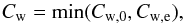 (22)where the adopted Cw,0 is presented in Sect. 2.6.
2.4. Temperature: viscous heating and radiative equilibrium
By referring to the terms concerning in Eq. (14), the viscous heating rate can be scaled as ~ . Since Σ decreases with t and
  has a negative dependence on r, the viscous heating is anticipated to play a primary role in determining the temperature in the inner region (≲10 au) and at the early stage of the evolution of a PPD. As Σ decreases with the dispersal of the gas component, the disc evolves passively by the illumination from the central star. A number of works have been published that treat this problem with detailed models that include viscous heating and stellar irradiation (e.g., Garaud & Lin 2007; Oka et al. 2011; Bitsch et al. 2015).
If the viscous heating is more effective in a PPD than stellar irradiation, then the temperature at the midplane, Tmid, will be higher than Tsurf in Eq. (13). On the other hand, if the viscous heating is ineffective and the stellar irradiation dominates, then Tsurf will be higher than Tmid. The radiative transfer needs to be solved to determine the vertical temperature profile. However, since our main focus here is to investigate the roles of magnetically driven disc winds, we adopt the simple prescription for the temperature that was introduced by Nakamoto & Nakagawa (1994). We defined Tvis as the temperature at the midplane determined by viscous heating, 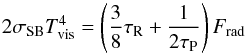 (23)where τR and τP are the Rosseland mean optical depth and the Planck mean optical depth measured at the midplane. τR is estimated from the surface density and the Rosseland mean opacity, κR, (Hueso & Guillot 2005) as
 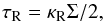 (24)where we use
  (25)based on the opacity of dust grains (Nakamoto & Nakagawa 1994, see also Baillié et al. 2015). The Planck mean optical depth can be approximated as
  (26)(Nakamoto & Nakagawa 1994; Hueso & Guillot 2005), where we give the lower bound on τP to obtain the pre-factor of Eq. (23),
  , for the optically thin limit.
We can also define the temperature under the radiation equilibrium, which is determined by the irradiation from the central star,  (27)We adopted T1au = 280 K and p = −1/2 based on the simple radiative equilibrium for the original minimum mass solar nebula (MMSN) (Hayashi 1981; Hayashi et al. 1985). We note that a slightly different scaling is derived, when the geometry of a flared disc is taken into account (Chiang & Goldreich 1997; Chiang & Youdin 2010).
When a PPD becomes optically thin and the viscous heating is ineffective, not only Tsurf but also Tmid approaches Treq. To take both viscous heating and stellar irradiation into account, we tool the sum of these two temperatures,  (28)for the representative z-averaged temperature, T, to estimate cs in Eq. (3).
2.5. Initial and boundary conditions
We calculated the evolution of Σ of the initial profile, ∝r− 3/2 (Hayashi 1981; Hayashi et al. 1985), with a cut-off radius rcut (29)The original MMSN by Hayashi (1981) considered Σ1au = 1.7 × 10³ g cm-2 with a sharp cut-off at 36 au, which gives the initial disc mass, Mdisc,int = 0.013 M⊙. We adopted a ten times larger Σ1au = 1.7 × 10⁴ g cm-2 but slightly smaller rcut = 30 au in this paper, which gives Mdisc,int = 0.11 M⊙. Mass accretion rates are observationally obtained as a function of time (Gullbring et al. 1998; Hartmann et al. 1998; Ricci et al. 2010; Manara et al. 2016), which corresponds to the age of the central stars, while the MMSN corresponds to a late stage of the evolution. Therefore, we chose the massive initial disc to directly compare our results to these observations.
We solved Eq. (10) to track the time evolution of Σ in the region from rin = 0.01 au to rout = 104 au with grid spacing,  . At the inner and outer boundaries, r = rin and = rout, we imposed
  , which corresponds to the zero-torque boundary condition (Lynden-Bell & Pringle 1974); the term in Eq. (10),
  , is zero for a constant and
  (Eq. (27) with p = −1/2).
2.6. Parameters
The free parameters of our model are turbulent viscosity, , disc wind mass flux, Cw,0, and disc wind torque, . We would like to note that, although we here call turbulent viscosity, large-scale magnetic fields possibly contribute to in realistic situations (Turner & Sano 2008; Johansen et al. 2009).
2.6.1. Turbulent viscosity – 
We compared two cases with spatially uniform  , and 8 × 10⁻⁵. was adopted from the result of local shearing box MHD simulations with sufficient ionization (Suzuki et al. 2010, see also e.g. Sano et al. 2004; Sai et al. 2013) in which MHD turbulence is fully developed by the MRI. When the ionization is not sufficient and non-ideal MHD effects such as resistivity, Hall diffusion, and ambipolar diffusion are important, a magnetically inactive dead zone forms (Gammie 1996) and is smaller (Sano et al. 1998; Lesur & Longaretti 2007; Simon et al. 2011; Okuzumi & Hirose 2011; Flock et al. 2012; Gressel et al. 2015). We adopted
  for such MRI-inactive circumstances. Although we assumed constant for simplicity, would be spatially dependent on r and evolve with time in realistic situations, because a dead zone generally forms only in the inner region and its size shrinks with time (e.g., Sano et al. 2000; Suzuki et al. 2010; Dzyurkevich et al. 2013). For future elaborate studies, we need to take this spatially and time-dependent into account.
2.6.2. Disc wind mass flux – Cw,0
The mass flux of disc winds, Cw,0, was also adopted from the local simulations. Cw,0 is controlled by the density at the wind onset region, which is located at the upper regions where the magnetic energy becomes comparable to the thermal energy. For the MRI turbulence, depending on the net vertical magnetic field, the density at the wind footpoint is ≈10-5−10-4 times the density at the midplane, which gives Cw,0 ≈ 10-5−10-4. Here, we add a note of caution: the local simulations might overestimate the mass-loss rate of the disc winds because the returning mass to the simulation box cannot be properly taken into account. Suzuki et al. (2010) reported that the mass flux is reduced by a factor of 2–3 in simulations with a larger vertical box size. Fromang et al. (2013) also pointed out that the reduction factor could be as large as ~10, but their numerical scheme and other detailed set-up were different from those used in Suzuki et al. (2010). These results show that we must choose Cw,0 carefully from the local simulations.
When we take the face value of the local simulations assuming the ideal MHD condition, Cw,0 ≈ 4 × 10⁻⁵ for the weak vertical magnetic field (Suzuki & Inutsuka 2009). We here set a more conservative value, Cw,0 = 2 × 10⁻⁵, for the MRI-active cases with . If a dead zone is formed, then the mass flux of the disc winds is slightly reduced, but it does not become as low as because the disc winds are driven from the surface regions with sufficient ionization; Cw,0 is only moderately weakened by a factor of a few. We adopted Cw,0 = 1 × 10⁻⁵ for . Moreover, the actual mass flux, Cw, is constrained by the energetics, Eq. (22). We also assumes, in the same way as , constant Cw,0 for simplicity. While in realistic situations it would depend on r and vary with time, it does not change as much as .
2.6.3. Disc wind torque – 
We tested two types of the parametrization for the wind torque: (i) constant  ; and (ii) density dependent with a cap,
 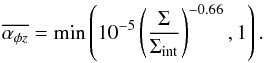 (30)We name (i) constant torque and (ii) Σ-dependent torque from now on. was estimated by local MHD simulations by Bai (2013), who reported
  with a positive dependence on the strength of the net vertical magnetic field,
  . ρmid is proportional to Σ, while Bz is determined by the inward dragging and outward diffusion of magnetic flux (Lubow et al. 1994; Okuzumi et al. 2014; Guilet & Ogilvie 2014, see also Sect. 4.4). If Bz decreases with the dispersal of gas (decrease of Σ), then will stay approximately constant, which corresponds to (i) constant torque; if Bz does not decrease that much, then has a negative dependence on Σ and will increase with time, which corresponds to (ii) Σ-dependent torque. We tested these two extreme limits for the effect of the wind torque affected by the evolution of the vertical magnetic flux.
3. Results
In this section, we present the properties of the time evolution of PPDs in the MRI-active and MRI-inactive conditions.
3.1. MRI-active cases
 |
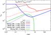
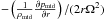
Fig. 1 Comparison of time evolutions of four MRI-active PPDs with |
In this subsection we show results of four cases of MRI-active PPDs, which are summarized in Table 1. The first three cases take disc winds into account. The magnetic braking by the disc winds is only considered in the first case. The last case (no DW) does not take disc winds into account by substituting ϵrad = 1 and Cw,0 = 0 in Eqs. (20)–(22).
Figure 1 compares radial profiles of T and Σ of these four cases. The top panel compares the evolution of the temperatures of these four cases. The initial temperature profiles in 0.1 au ≲ r ≲ 5 au, are kept more or less constant ≲1500−2500 K because dust grains sublimate and the opacity drops above that temperature (Eq. (25); see also Baillié et al. 2015). Furthermore, the initial profiles are almost the same for the four cases, except for different energetics constraints on Cw and wind torques, . In particular, the weak DW case (adopting Eqs. (20) and (21); purple dotted line) gives a very similar profile to those of the strong DW cases (adopting Eqs. (18) and (19); red and green dotted line), which needs explanation. In the inner region, ≲10 au, T ≈ Tvis (Eq. (28)) in these cases, and then T is mainly determined from Frad by Eq. (23). Recalling Σint ∝ r− 3/2, we derive 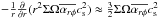 for
for  . Since the (0 or =10-5) term in Eq. (21) is negligible in comparison to the
  term, both strong DW and weak DW conditions give similar Frad in Eqs. (19) and (21), and accordingly, the initial temperatures of these cases are similar each other.
In the no DW case (black lines) the viscous heating region (Tvis>Treq) survives until a later time although its size shrinks. In contrast, the temperatures decrease more rapidly in the other cases with disc winds. In the two strong DW cases (red and green lines), the temperatures are mainly determined by Treq in the entire region after t ≳ 106 yr because the surface densities decrease rapidly by the disc winds in the inner region to give Treq ≫ Tvis, while Tvis is no longer negligible in the weak DW case (purple lines) at t = 106 yr.
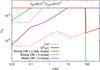 |
Fig. 2 Comparison of nondimensional mass flux of disc winds, Cw, of the three MRI-active cases except for the no DW case in Table 1. at t = 0 (dotted lines) and 106 yr (solid lines). |
The bottom panel of Fig. 1 compares the evolution of the surface densities. The disc winds reduce Σ particularly in small r regions (Suzuki et al. 2010). A comparison between the two zero-torque cases (green and purple lines) shows the difference between the strong DW and weak DW conditions. As expected, the strong DW case shows faster decrease of Σ because of the higher disc wind mass flux, Cw, which is shown in Fig. 2. At t = 0 the strong DW case (green dotted line) gives quite small Cw ≈ 0 below the displayed range of Fig. 2 because  for Σint ∝ r− 3/2 in Eq. (18). However, as Σ decreases in an inside-out manner and the Σ profile changes, Cw increases and at t = 106 yr this case (green solid line) yields larger Cw than the weak DW case (purple solid line), in which Cw instead decreases with time owing to the decrease in temperature (∝
 ; Eq. (21)). We note that Cw = 0 in the outer region, r> 90 au, of the strong DW + zero-torque case because the gas moves outward (
 in Eq. (18)) in the outer region and the gravitation energy is not released. In realistic situations, however, a moderate level of external heating by stellar irradiation or other sources would cause disc winds to be launched by relaxing the energetics constraint (see Sect. 4.1), because the gas is only weakly bound by the gravity in the outer region.
Parameters for MRI-active cases.
The non-zero wind torque also reduces Σ faster (red lines in the bottom panel of Fig. 1) by the enhanced accretion and disc wind mass-loss. A comparison between the red and green lines in Fig. 2 indicates that the removal of angular momentum by the φz stress additionally contributes to the gravitational energy by the accretion to enhance Cw (Eq. (18)). As a result, Cw is not constrained by the energetics, Cw,e, in the almost entire region but is determined by Cw,0( = 2 × 10⁻⁵) at t = 106 yr (red solid lines). The constant Cw = Cw,0 implies faster dispersal of Σ for smaller r because the mass-loss timescale becomes proportional to the Keplerian time (Suzuki et al. 2010; Ogihara et al. 2015a,b), and the slope of Σ is positive in the inner region. The slope of Σ is again negative in the very inner region, r< 0.1 au, at later time, t ≳ 107 yr. This is because is constrained by the cap value = 1 (Eq. (30) there.
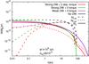 |
Fig. 3 Mass-loss rate by disc wind, Ṁz, (solid lines) and mass accretion rate induced by the rφ stress, Ṁr,rφ (dashed lines) and by the φz stress, Ṁr,rφ (dotted lines) at t = 106 yr of the four MRI-active cases in Table 1. Ṁz = 0 for the no DW case and Ṁr,φz = 0 for the zero-torque cases. |
Figure 3 presents the radial profile of the mass-loss rate by disc winds (solid lines),  (31)and the mass accretion rate,
  (32)at t = 106 yr. Here, Ṁr can be separated into two parts, Ṁr = Ṁr,rφ + Ṁr,φz, following Eq. (5) with help of Eqs. (6) and (8) (see also Simon et al. 2013): mass accretion induced by the rφ stress (dashed lines),
 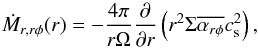 (33)and that by the φz stress (dotted line)
 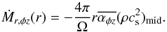 (34)We note that Ṁz(r) in our definition is the total mass loss outside r, while the disc wind mass loss at r is sometimes defined as the mass lost inside r (e.g., Owen et al. 2011; Bai et al. 2016; Bai 2016). We chose our definition to show how
  is converted into Ṁz as mass accretes inward.
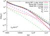 |
Fig. 4 Time evolution of Ṁz (solid) and Ṁr = Ṁr,rφ + Ṁr,φz (dashed) at r = 0.0225 au of the four MRI-active cases in Table 1. |
The no DW case shows a spatially uniform accretion rate, Ṁr,rφ = 1.5 × 10⁻⁸M⊙ yr-1 in r< 10 au (black dashed line). When disc winds are taken into account, the mass accretion rate decreases with decreasing r as the mass is lost by the disc winds. When we evaluate Ṁ at r = 0.0225 au (≈4.8 R⊙), which is one grid point outside rin = 0.01 au and approximately twice the radius of typical T Tauri stars, Ṁr,rφ is reduced to 2.5 × 10⁻⁹M⊙ yr-1 in the weak DW case (purple dashed line). Instead, the mass is largely lost by the disc winds, Ṁz = 1.0 × 10⁻⁸M⊙ yr-1 at r = 0.0225 au (purple solid line). This situation is more drastic in the strong DW + zero-torque case, and Ṁz ≈ 100Ṁr,rφ (green lines) at r = 0.0225 au. We note that Ṁ might have to be evaluated at a slightly outer location when the inner disc is truncated by the magnetosphere of the central star (e.g., Shu et al. 1994; Hirose et al. 1997; Dyda et al. 2015); in this case, Ṁr is not as small as the above evaluated values.
The strong DW + Σ-dependent torque case (red lines) gives very small Ṁr,rφ at r = 0.0225 au because Σ is small there (Fig. 1). On the other hand, the accretion by the φz stress is non-zero only in this case of the four cases displayed in Fig. 3, and Ṁr,φz is still kept = 2.4 × 10⁻⁹M⊙ yr-1 at r = 0.0225 au because increases to ≈0.1 in the inner region; the disc is in a wind-driven accretion phase.
Figure 4 compares the time evolutions of Ṁz (solid) and Ṁr = Ṁr,rφ + Ṁr,φz (dashed) at r = 0.0225 au of these four cases. The obtained t−Ṁr trends can be directly compared to the observed distribution in the t−Ṁr plane (Gullbring et al. 1998; Hartmann et al. 1998; Ricci et al. 2010; Manara et al. 2016). Although Ṁr of the strong DW + zero-torque case is smaller than the observed lower edge (Ṁr ~ 10-9M⊙ yr-1 at t = 106 yr), Ṁr of the other three cases are well inside the observed range.
3.2. MRI-inactive cases
Parameters for MRI-inactive cases.
 |
Fig. 5 Same as Fig. 1 but for four MRI-inactive cases with |
We present results of four MRI-inactive cases, which are summarized in Table 2. We focus on effects of the wind torque on the evolution of PPDs in this subsection. Figure 5 compares radial profiles of T and Σ. The temperatures (top panel) of these cases are systematically lower than the temperatures of the MRI-active cases (the top panel of Fig. 1) because smaller gives smaller Frad (Eqs. (19) and (21)) and accordingly lower Tvis (Eq. (23)).
Smaller also leads to slower evolution; when the MRI-active and MRI-inactive cases are compared, which adopt the same strong DW + zero-torque parameters (green lines in Figs. 1 and 5), the decrease of Σ is much slower in the MRI-inactive case. This is first because the accretion itself is slower owing to the smaller and second because the disc wind mass flux is strongly constrained by the energetics to give smaller Cw (Fig. 6 in comparison to Fig. 2).
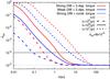 |
Fig. 7 Comparison of |
The evolution of Σ is largely affected by non-zero wind torque , because its effect is relatively important for lower turbulent viscosity, . The addition of the spatially constant  (constant torque, grey lines) greatly reduces Σ. The two Σ-dependent torque cases (red and blue lines) give positive slopes of Σ in the inner region, which we explain below.
Figure 7 presents the time evolution of for the Σ-dependent torque cases. increases with time from the inside to the outside as Σ decreases in an inside-out manner. As a result, the disc wind mass flux, Cw, is not constrained by the energetics (Eqs. (18) and (20)) but is chosen to be the constant Cw,0( = 10-5) in Eq. (22) (Fig. 6), which leads to the inside-out dispersal of the gas. In addition, the accretion is faster for smaller r because is larger for smaller r. The positive slopes of Σ can be explained by the combination of these effects.
Although we assumed spatially uniform and Cw,0, they are also anticipated to depend on the strength of net vertical magnetic field,  . In this case, and Cw,0 could inversely correlate with Σ (Suzuki et al. 2010), which additionally enhances the positive slopes of the surface densities.
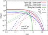
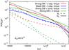
Figure 8 compares Ṁz (Eq. (31); solid), Ṁr,rφ (Eq. (33); dashed), and Ṁr,φz (Eq. (34); dotted) of the MRI-inactive four cases at t = 106 yr. In the zero-torque case (green lines) the mass is dominantly lost by the disc winds, Ṁz ≈ 100Ṁr,rφ at r = 0.0225 au. In the constant torque case (grey lines) the mass accretion is mainly driven by the φz stress, the total accretion rate is also largely dominated by the mass loss by the disc winds. Adopting the Σ-dependent torque condition changes the situation; the mass accretion is driven by the φz stress, and the accretion rate is well above 10-9M⊙ yr-1, that is, the weak DW case gives Ṁr,φz ≈ Ṁz ≈ 5 × 10⁻⁹M⊙ yr-1 at r = 0.0225 au.
Figure 9 shows the time evolution of Ṁz (solid) and Ṁr = Ṁr,rφ + Ṁr,φz (dashed) at r = 0.0225 au of the same four cases. Ṁr(0.0225 au) of the cases of zero or constant torque (green and grey dashed lines) are smaller than the observed range of t−Ṁr (Gullbring et al. 1998; Hartmann et al. 1998; Ricci et al. 2010; Manara et al. 2016). On the other hand, Ṁr(0.0225au)’s of the Σ-dependent torque cases (red and blue dashed lines) are consistent with the observed t−Ṁr. Although the mass accretion rate of the strong DW case is lower than the wind mass-loss rate (red lines), it is not so small; Ṁr(0.0225 au) = 6.0 × 10⁻⁹M⊙ yr-1 at t = 105 yr, 1.7 × 10⁻⁹M⊙ yr-1 at 106 yr, and 5.2 × 10⁻¹⁰M⊙ yr-1 at 107 yr.
4. Discussion
4.1. Uncertainties
Our model has the three free parameters, , Cw,0, and . Since these parameters are not yet tightly constrained by observations or theoretical calculations, we calculated the evolution of PPDs in the wide ranges of the parameters to test various possibilities (Sect. 3). Uncertainties of the three parameters is largely attributed to the uncertainty of the initial distribution and to the evolution of the poloidal magnetic flux because these three parameters depend on the vertical magnetic field strength (Suzuki et al. 2010; Okuzumi & Hirose 2011; Bai & Stone 2013b).
The evolution of poloidal magnetic flux in accretion discs has been studied by a number of groups (Lubow et al. 1994; Rothstein & Lovelace 2008; Guilet & Ogilvie 2012; Suzuki & Inutsuka 2014) and has recently been specifically applied to PPDs (Okuzumi et al. 2014; Guilet & Ogilvie 2014; Takeuchi & Okuzumi 2014). Accreting gas drags the vertical magnetic field inward, while the vertical field also possibly diffuses outward by magnetic diffusivity, which consists of both effective turbulent resistivity and non-ideal MHD effects (Sect. 2.6). The radial motion of the vertical magnetic flux is determined by the balance between these inward dragging and outward diffusion. The direction of the magnetic flux itself is still uncertain, which depends on the initial configuration of the poloidal magnetic field, in addition to the combination of accretion and magnetic diffusion.
One future possibility is that we finally obtain a universal tendency for the time evolution of vertical magnetic fields. In this case, we can constrain our free parameters, and evolutions of surface densities will not show a variety but converge to a unified trend. On the other hand, if the evolution of the poloidal magnetic flux is different in different PPDs, depending on physical circumstances, such as initial magnetic flux and disc mass, and stellar irradiation, which controls the non-ideal MHD effects through the ionization, then the evolutions of surface densities are also different in different PPDs as shown so far, which should lead to a wide variety of the subsequent planet formation processes and final exoplanet systems.
At present, the unified picture of the evolution of the poloidal magnetic field is not well understood at all, and therefore it is worth pursuing various possibilities. Our calculations took the effect of the evolution of the vertical magnetic field in the wind torque into account; the two cases of constant and Σ-dependent correspond to the case in which the magnetic energy decreases in the same manner as the decrease of the surface density and the case with the preserved magnetic flux, respectively. The Σ-dependent torque cases show a runaway behavior of the gas dispersal in an inside-out manner; once the gas is dispersed, increases, which further accelerates the dispersal of the gas. This is the main reason why the positive slope of Σ is produced. Although we did not consider this effect, and Cw,0 depend similarly on Σ, which causes an additional runaway dispersal of the gas (Suzuki et al. 2010, see also Sect. 3.2). The case with constant even gives the moderately positive slope (Fig. 5). Within the two cases we tested, the positive slope of Σ on r is not peculiar, but a common feature. However, we should note that our calculations do not cover all the possible distributions and evolutions of the vertical magnetic field. Therefore, it would be premature to conclude that the positive slope of Σ is a natural outcome of the accretion induced by the magnetically driven disc wind. For example, when the outward diffusion of vertical magnetic field is effective and the magnetic flux is dispersed more rapidly than the gas, the effect of the wind torque is suppressed with time. In this case, the Σ profile would maintain a normal negative slope.
We now discuss other ambiguities of the mass flux of the disc winds, in addition to the uncertainty of the vertical magnetic field. At the moment, the mass flux, Cw,0, is available only from local MHD simulations (e.g. Suzuki & Inutsuka 2009; Fromang et al. 2013; Bai & Stone 2013a). As discussed in Sect. 2.6, these local simulations may overestimate the mass flux. Although we adopted the conservative Cw,0 by reducing the simulation results by half (see Sect. 2.6), it might be even lower (Fromang et al. 2013). We here briefly discuss how the results are affected and particularly focus on the slope of the surface density when Cw,0 is smaller.
As shown in Figs. 2 and 6,Cw is already constrained by the energetics. In most cases except for the MRI-inactive cases with Σ-dependent torque, the energetics constraint already suppresses Cw in the inner region. Therefore, adopting a smaller Cw,0 does not affect Cw in the inner region but reduces Cw in the outer region, which suppresses the gas dispersal there. Hence, the slope of Σ would be more positive in these cases. On the other hand, in the MRI-inactive cases with Σ-dependent torque, the energetics constraint suppresses Cw at the relatively outer location, r ~ 10 au. In these cases, a smaller Cw,0 reduces Cw in the inner region. As a result, the obtained large positive Σ slopes in these cases (Fig. 6) would be reduced to moderately positive ones.
When we determined the mass flux of the disc winds, we applied the energetics constraint from the gravitational accretion without external heating or momentum inputs (Sect. 2.3; Eq. (22)). This treatment is expected to give a reasonable constraint at the early phase when viscous heating dominates the radiative heating or other effects from the central star. However, at the later time this is not the case because the surface density decreases and the viscous heating becomes relatively unimportant. Effects of external heating or momentum inputs need to be considered. They weaken the energetics constraint to give a larger Cw in the region with Cw,e<Cw,0 (see Sect. 4.5).
4.2. Radial drift of pebbles and boulders
Although calculations still include uncertainties that mainly stem from the ambiguity of the evolution of poloidal magnetic fields, the positive slopes of the surface densities obtained in Sect. 3 are a possible consequence of the evolution of PPDs with disc winds, as discussed in Sect. 4.1. These positive slopes raise various interesting implications for planet formation. In this and the next subsections, we demonstrate how the obtained Σ profiles affect the solid component of PPDs by studying cases that show large positive slopes of Σ.
The first example is the radial drift of solid bodies through gas drag. In general the rotation velocity of the gas in PPDs is slightly slower than the local Keplerian velocity because of the radial pressure gradient force. On the other hand, solid particles rotate with Keplerian velocity without the support from the gas pressure. As a result, the solid particles feel a head wind from the gas, which causes them to drift inward. Considering the momentum balance, solid particles with nondimensional stopping time ≈1, which corresponds to a meter-sized spherical boulder at 1 au of the MMSN, experience the radial drift most severely (Weidenschilling 1977; Nakagawa et al. 1986), and their drift timescale in the midplane is given by 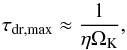 (35)where η is pressure gradient force normalized by the twice of centrifugal force,
 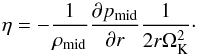 (36)In the usual condition, η ~ 10-3−10-2> 0, which causes solid particles to drift inward. Smaller η leads to slower inward drift; if η< 0, the direction of the drift is opposite and solid particles move outward.
Figure 10 shows η of the two MRI-inactive ( ) cases with Σ-dependent torque of Table 2 (red and blue lines; the same as in Figs. 5–9) in comparison to the no disc wind (no DW) case with the same (black lines). We here derive pmid from Σ by
 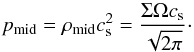 (37)The no DW case shows η remains within 10-3−10-2, which implies fast inward drift. In contrast, η’s are considerably reduced in the Σ-dependent torque cases. In particular, the red lines (strong DW case) show negative η in part (red lines are truncated between 0.04–0.4 au at t = 105 yr and 1–2 au at t = 106 yr), which indicates that solid particles move outward in this region. As a result, the solid component will accumulate around the outer edge of the negative η region, which offers suitable conditions for planet formation (Kobayashi et al. 2012). Furthermore, this location moves outward with time; the suitable site for the planet formation also moves outward.
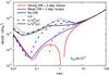 |
Fig. 10 Comparison of normalized pressure gradient force, |
4.3. Type I migration
 |
Fig. 11 Migration efficiency for Earth-mass planets for MRI-inactive cases with Σ-dependent torque (red for strong DW and blue for weak DW of Table 2) at t = 106 yr (corresponding to the solid red and blue lines in Fig. 5) in comparison to the MRI-inactive no DW case (black). CI > 0 means outward migration. |
Another interesting implication of the positive Σ slopes is that an inward migration of low-mass planets (type I migration) can be slowed down or even reversed. The torque for type I migration can be expressed by the sum of Lindblad and corotation torques. The corotation torque is more sensitive to the slope of the gas surface density and can be positive for positive slopes.
Here we estimate the migration rate of Earth-mass planets embedded in MRI-inactive PPDs with the surface densities shown in Fig. 5. We used the formulae of Paardekooper et al. (2011) to calculate the migration timescale, ta (see Eqs. (8)–(16) in Ogihara et al. (2015a) for details of the formulae). We introduced a parameter of the efficiency of inward type I migration, CI ≡ −ta,TTW/ta, where ta,TTW is the migration time in a locally isothermal disc derived by a linear analysis by Tanaka et al. (2002). The migration timescale is defined as ta ≡ a/ (−ȧ); positive migration time means inward migration.
Figure 11 shows the migration efficiency for the Σ-dependent torque case (the red and blue curves in Fig. 5) at t = 106 yr in comparison to the no DW case (black line). The migration rate depends on the planetary mass and the orbital eccentricity; Earth-mass planets with zero eccentricity were considered here. The blue curve shows that the type I migration is slowed down inside a few au by several factors from ta,TTW. The migration is even reversed (outward migration) between 0.1–0.5 au in the red curve (strong DW case). Thus the disc wind would also play important roles in the late stage of planet formation.
4.4. Comparison to previous work
Recently, Bai (2016) also presented a global evolution model for PPDs with magnetically driven disc winds. However, none of the cases in his model calculations resulted in a surface density with a drastic positive slope relative to r as some of our cases have shown. The two main differences between his setup and ours is the mass-loss rate by the disc wind and the evolution of the vertical magnetic field.
Our calculations, which started from a relatively massive initial disc (Mdisc,int = 0.11 M⊙) to study the evolution from the early stage, neglected the heating by the irradiation from a central star but considered viscous heating, and the mass-loss rate was constrained by the global energetics of the viscous accretion. In contrast, the initial disc mass adopted by Bai (2016) is lower, =0.035 M⊙, to focus on the later stage of the evolution, and the location of the wind base in the inner region r ≲ 10−30 au is determined from heating by far-ultraviolet (FUV) irradiation from a central star. Here, the penetration depth of the FUV was assumed to be spatially constant. Since the surface density decreases with r, the penetration depth normalized by the scale height is deeper for larger r. Therefore, the mass loss by the disc wind affects the depletion of the gas at outer locations more severely than in our model setting, and consequently a positive slope of Σ was not obtained in the results of Bai (2016).
As for the evolution of the vertical magnetic field, Bai (2016) considered two cases: in the first case the total magnetic flux is preserved with time, and in the second case it decreases in the same manner as the total mass. In both cases, the plasma  at the midplane was assumed to be spatially uniform. Even in the first case, the vertical magnetic field was redistributed to follow the density profile (Armitage et al. 2013). This spatially uniform β was also adopted in our constant torque setting. In contrast, our Σ-dependent torque assumed the preserved vertical magnetic field at each location, which led to a runaway inside-out dispersal and produced a large positive slope of Σ (Sect. 3), compared to the above-mentioned cases with the spatially uniform β.
4.5. Stellar wind and photoevaporation
We did not take the effects of a central star into account except to determine the radiative equilibrium temperature, Treq (Eq. (27)). However, the stellar wind and irradiation affect the evolution of PPDs.
In our calculations, the mass flux of the disc wind is Cw,e constrained by the energetics of accretion, and it can be smaller than Cw,0 determined by the mass loading expected from the local MHD simulations. When this is the case, gaseous clouds are lifted up by vertical upflows but cannot stream out to large z; they float in the disc atmosphere or return to the disc because they are bound by the gravity of the central star. The stellar wind from the central star would change this situation.
The mass flux of the stellar wind from pre-main sequence stars is much higher, by an order of 4–6, than that of the current solar wind partly because of the energy supply from accretion (Hirose et al. 1997; Matt & Pudritz 2005; Cranmer 2009). Even after the accretion terminates, the mass flux of the stellar wind is expected to be still high because of the high magnetic activity (Wood et al. 2005; Cranmer & Saar 2011; Suzuki et al. 2013). The strong stellar wind would blow away the clouds that are lifted up by the disc winds (see Suzuki et al. 2010, for the energetics). In the framework of our model, the contribution from the stellar wind would increase Cw,e in Eqs. (16) and (17), in the small r region. The increase of Cw in the inner region reduces Σ there, which also produces a larger positive slope of Σ.
In this discussion, we neglected the roles of global magnetic fields that are rooted in the central star and in the PPD. When the field strength is strong enough, the stellar wind region and the disc wind region are separated by a boundary layer formed by magnetospheric ejections (Zanni & Ferreira 2013). In this case the stellar winds will not contribute to driving the disc winds. It depends on the relative strength of the magnetic energy to the sum of the dynamic pressure and the gas pressure whether the interaction between the stellar winds and the disc winds is efficient. When the magnetic energy is weaker, the interaction is stronger, and vice versa.
Photoevaporation by irradiation from the central star or neighbouring stars has been extensively studied as a viable source for dispersing PPDs (e.g., Shu et al. 1993; Hollenbach et al. 2000; Adams et al. 2004). The mass-loss rate by the photoevaporation, which depends on the flux in different spectral ranges, FUV, extreme UV, and X-rays, yields a wide variety of ~10-10−10-8M⊙ yr-1 (Alexander et al. 2006; Ercolano et al. 2008; Gorti & Hollenbach 2009; Owen et al. 2010; Tanaka et al. 2013). After the mass accretion rate or the mass-loss rate by the disc wind decreases below this level, the photoevaporation would quickly disperse PPDs (e.g. Armitage 2011); our results would be affected at the late stage of the evolution.
However, we expect that the evolution of the Σ profile of a photoevaporating PPD is qualitatively different from our results with the magnetically driven disc wind because the photoevaporation mostly affects the disc dispersal in the outer region where the sound speed of the heated gas exceeds the local escape velocity from the central star. Although the photoevaporation could create an inner hole by the combination with the viscous accretion, the local slope of Σ remains negative except at the inner edge of the hole (e.g. Alexander et al. 2006; Owen et al. 2011). This is in clear contrast to the evolution with the magnetically driven disc wind.
5. Summary
We have studied the global evolution of PPDs by considering viscous heating and magnetically driven disc winds. We constructed a global model from fundamental MHD equations for the time-evolution of PPDs. One of the key features of our model is that the mass-loss rate by the disc wind is derived from both the local MHD shearing box simulations and the global energetics of the gravitational accretion. Our model has three dimensionless parameters, which are turbulence viscosity, , disc wind mass flux, Cw, and disc wind torque, , and these three parameters are constrained by the above-mentioned global energetics. We performed model calculations in a wide parameter range to cover both MRI-active PPDs and MRI-inactive PPDs with dead zones.
We started our calculations from the relatively massive disc, Mdisc.int = 0.11 M⊙. Initially, the viscous heating dominantly determines the temperature in the inner region <10 au; for instance, T ≃ 1500 K at 1 au, which is much higher than the temperature estimated from the radiative equilibrium. As the surface density decreases with time, the temperature approaches the radiative equilibrium temperature. In the cases that consider the disc wind mass loss, the gas in the inner region is rapidly dispersed before 106 yr, and the viscous heating is negligible in determining the temperature after t ≳ 106 yr, whereas in the no disc wind cases the viscous heating is not negligible even up to several 106 yr.
The mass accretion rates decrease with time as the surface densities decrease, regardless of whether the accretion is induced by turbulent viscosity or wind torque. The obtained accretion rates are consistent with observed accretion rates for a wide range of the adopted parameters.
The three free parameters, , Cw,0, and still contain ambiguities, arising mainly from the uncertainty of the evolution of vertical magnetic fields. We have pursued various possibilities by testing different combinations of these parameters. The detailed profiles of the temperatures and the surface densities show a wide variety. Since physical properties of a PPD affect planet formation processes that take place in the disc (e.g., Kobayashi et al. 2016), the obtained variety of our PPD calculations would be a source of the observed variety of exoplanet systems (e.g. Howard et al. 2012).
The wind-driven accretion can promote an increase in disc surface density with r in the inner region; this is the case in our calculations for MRI-inactive PPDs when the distribution of the vertical magnetic flux is preserved with time evolution (Sect. 3.2). This large positive slope of the surface density suppresses or reverses the inward drift of pebble- or boulder-sized solids through gas drag (Sect. 4.2) and the inward migration of protoplanets (Sect. 4.3), which is a favourable condition for the planet formation.
Acknowledgments
T.K.S. is supported by the Astrobiology Center Project of National Institute of Natural Sciences (NINS) (Grant Number AB271020, AB281018). A.M., A.C. and T.G. acknowledge support by the French ANR, project number ANR-13–13-BS05-0003-01 project MOJO (Modeling the Origin of JOvian planets). T.K.S. thanks Hiroshi Kobayashi and Shinsuke Takasao for fruitful discussions. The authors thank the referee for many valuable comments.
References
- Adams, F. C., Hollenbach, D., Laughlin, G., & Gorti, U. 2004, ApJ, 611, 360 [NASA ADS] [CrossRef] [Google Scholar]
- Alexander, R. D., Clarke, C. J., & Pringle, J. E. 2006, MNRAS, 369, 229 [NASA ADS] [CrossRef] [Google Scholar]
- Armitage, P. J. 2011, ARA&A, 49, 195 [NASA ADS] [CrossRef] [EDP Sciences] [Google Scholar]
- Armitage, P. J., Simon, J. B., & Martin, R. G. 2013, ApJ, 778, L14 [NASA ADS] [CrossRef] [Google Scholar]
- Bai, X.-N. 2013, ApJ, 772, 96 [NASA ADS] [CrossRef] [Google Scholar]
- Bai, X.-N. 2016, ApJ, 821, 80 [NASA ADS] [CrossRef] [Google Scholar]
- Bai, X.-N., & Stone, J. M. 2013a, ApJ, 767, 30 [NASA ADS] [CrossRef] [Google Scholar]
- Bai, X.-N., & Stone, J. M. 2013b, ApJ, 769, 76 [NASA ADS] [CrossRef] [Google Scholar]
- Bai, X.-N., Ye, J., Goodman, J., & Yuan, F. 2016, ApJ, 818, 152 [Google Scholar]
- Baillié, K., Charnoz, S., & Pantin, E. 2015, A&A, 577, A65 [NASA ADS] [CrossRef] [EDP Sciences] [Google Scholar]
- Balbus, S. A., & Hawley, J. F. 1991, ApJ, 376, 214 [NASA ADS] [CrossRef] [Google Scholar]
- Balbus, S. A., & Hawley, J. F. 1998, Rev. Mod. Phys., 70, 1 [Google Scholar]
- Bitsch, B., Johansen, A., Lambrechts, M., & Morbidelli, A. 2015, A&A, 575, A28 [NASA ADS] [CrossRef] [EDP Sciences] [Google Scholar]
- Blandford, R. D., & Payne, D. G. 1982, MNRAS, 199, 883 [NASA ADS] [CrossRef] [Google Scholar]
- Chandrasekhar, S. 1961, Hydrodynamic and hydromagnetic stability (Oxford: Clarendon) [Google Scholar]
- Chiang, E., & Youdin, A. N. 2010, Ann. Rev. Earth Planet. Sci., 38, 493 [Google Scholar]
- Chiang, E. I., & Goldreich, P. 1997, ApJ, 490, 368 [NASA ADS] [CrossRef] [Google Scholar]
- Cranmer, S. R. 2009, ApJ, 706, 824 [NASA ADS] [CrossRef] [Google Scholar]
- Cranmer, S. R., & Saar, S. H. 2011, ApJ, 741, 54 [NASA ADS] [CrossRef] [Google Scholar]
- Davis, S. S. 2005, ApJ, 620, 994 [NASA ADS] [CrossRef] [Google Scholar]
- Dullemond, C. P., van Zadelhoff, G. J., & Natta, A. 2002, A&A, 389, 464 [NASA ADS] [CrossRef] [EDP Sciences] [Google Scholar]
- Dyda, S., Lovelace, R. V. E., Ustyugova, G. V., et al. 2015, MNRAS, 450, 481 [NASA ADS] [CrossRef] [Google Scholar]
- Dzyurkevich, N., Turner, N. J., Henning, T., & Kley, W. 2013, ApJ, 765, 114 [NASA ADS] [CrossRef] [Google Scholar]
- Ercolano, B., Drake, J. J., Raymond, J. C., & Clarke, C. C. 2008, ApJ, 688, 398 [NASA ADS] [CrossRef] [Google Scholar]
- Ferreira, J., Dougados, C., & Cabrit, S. 2006, A&A, 453, 785 [NASA ADS] [CrossRef] [EDP Sciences] [Google Scholar]
- Flock, M., Henning, T., & Klahr, H. 2012, ApJ, 761, 95 [NASA ADS] [CrossRef] [Google Scholar]
- Fromang, S., Latter, H., Lesur, G., & Ogilvie, G. I. 2013, A&A, 552, A71 [NASA ADS] [CrossRef] [EDP Sciences] [Google Scholar]
- Gammie, C. F. 1996, ApJ, 457, 355 [NASA ADS] [CrossRef] [Google Scholar]
- Garaud, P., & Lin, D. N. C. 2007, ApJ, 654, 606 [Google Scholar]
- Gorti, U., & Hollenbach, D. 2009, ApJ, 690, 1539 [Google Scholar]
- Gressel, O., Turner, N. J., Nelson, R. P., & McNally, C. P. 2015, ApJ, 801, 84 [NASA ADS] [CrossRef] [Google Scholar]
- Guilet, J., & Ogilvie, G. I. 2012, MNRAS, 424, 2097 [NASA ADS] [CrossRef] [Google Scholar]
- Guilet, J., & Ogilvie, G. I. 2014, MNRAS, 441, 852 [NASA ADS] [CrossRef] [Google Scholar]
- Gullbring, E., Hartmann, L., Briceño, C., & Calvet, N. 1998, ApJ, 492, 323 [NASA ADS] [CrossRef] [Google Scholar]
- Haisch, Jr., K. E., Lada, E. A., & Lada, C. J. 2001, ApJ, 553, L153 [NASA ADS] [CrossRef] [Google Scholar]
- Hartmann, L., Calvet, N., Gullbring, E., & D’Alessio, P. 1998, ApJ, 495, 385 [NASA ADS] [CrossRef] [Google Scholar]
- Hawley, J. F., Guan, X., & Krolik, J. H. 2011, ApJ, 738, 84 [NASA ADS] [CrossRef] [Google Scholar]
- Hayashi, C. 1981, Prog. Theor. Phys. Suppl., 70, 35 [NASA ADS] [CrossRef] [MathSciNet] [Google Scholar]
- Hayashi, C., Nakazawa, K., & Nakagawa, Y. 1985, in Protostars and Planets II, eds. D. C. Black, & M. S. Matthews (Tucson: The University of Arizona Press), 1100 [Google Scholar]
- Hernández, J., Hartmann, L., Calvet, N., et al. 2008, ApJ, 686, 1195 [NASA ADS] [CrossRef] [Google Scholar]
- Hirose, S., & Turner, N. J. 2011, ApJ, 732, L30 [NASA ADS] [CrossRef] [Google Scholar]
- Hirose, S., Uchida, Y., Shibata, K., & Matsumoto, R. 1997, PASJ, 49, 193 [Google Scholar]
- Hollenbach, D. J., Yorke, H. W., & Johnstone, D. 2000, Protostars and Planets IV (Tucson: The University of Arizona Press), 401 [Google Scholar]
- Howard, A. W., Marcy, G. W., Bryson, S. T., et al. 2012, ApJS, 201, 15 [NASA ADS] [CrossRef] [Google Scholar]
- Hueso, R., & Guillot, T. 2005, A&A, 442, 703 [NASA ADS] [CrossRef] [EDP Sciences] [Google Scholar]
- Johansen, A., Youdin, A., & Klahr, H. 2009, ApJ, 697, 1269 [NASA ADS] [CrossRef] [Google Scholar]
- Kimura, S. S., Kunitomo, M., & Takahashi, S. Z. 2016, MNRAS, 461, 2257 [NASA ADS] [CrossRef] [Google Scholar]
- Kobayashi, H., Ormel, C. W., & Ida, S. 2012, ApJ, 756, 70 [NASA ADS] [CrossRef] [Google Scholar]
- Kobayashi, H., Tanaka, H., & Okuzumi, S. 2016, ApJ, 817, 105 [NASA ADS] [CrossRef] [Google Scholar]
- Kusaka, T., Nakano, T., & Hayashi, C. 1970, Prog. Theor. Phys., 44, 1580 [NASA ADS] [CrossRef] [Google Scholar]
- Lesur, G., & Longaretti, P.-Y. 2007, MNRAS, 378, 1471 [NASA ADS] [CrossRef] [Google Scholar]
- Lesur, G., Ferreira, J., & Ogilvie, G. I. 2013, A&A, 550, A61 [NASA ADS] [CrossRef] [EDP Sciences] [Google Scholar]
- Lubow, S. H., Papaloizou, J. C. B., & Pringle, J. E. 1994, MNRAS, 267, 235 [NASA ADS] [Google Scholar]
- Lynden-Bell, D., & Pringle, J. E. 1974, MNRAS, 168, 603 [NASA ADS] [CrossRef] [Google Scholar]
- Manara, C. F., Fedele, D., Herczeg, G. J., & Teixeira, P. S. 2016, A&A, 585, A136 [NASA ADS] [CrossRef] [EDP Sciences] [Google Scholar]
- Matt, S., & Pudritz, R. E. 2005, ApJ, 632, L135 [NASA ADS] [CrossRef] [Google Scholar]
- Miyake, T., Suzuki, T. K., & Inutsuka, S.-I. 2016, ApJ, 821, 3 [NASA ADS] [CrossRef] [EDP Sciences] [Google Scholar]
- Nakagawa, Y., Sekiya, M., & Hayashi, C. 1986, ICARUS, 67, 375 [Google Scholar]
- Nakamoto, T., & Nakagawa, Y. 1994, ApJ, 421, 640 [NASA ADS] [CrossRef] [Google Scholar]
- Ogihara, M., Kobayashi, H., Inutsuka, S.-I., & Suzuki, T. K. 2015a, A&A, 579, A65 [NASA ADS] [CrossRef] [EDP Sciences] [Google Scholar]
- Ogihara, M., Morbidelli, A., & Guillot, T. 2015b, A&A, 584, L1 [NASA ADS] [CrossRef] [EDP Sciences] [Google Scholar]
- Oka, A., Nakamoto, T., & Ida, S. 2011, ApJ, 738, 141 [NASA ADS] [CrossRef] [Google Scholar]
- Okuzumi, S., & Hirose, S. 2011, ApJ, 742, 65 [NASA ADS] [CrossRef] [Google Scholar]
- Okuzumi, S., Takeuchi, T., & Muto, T. 2014, ApJ, 785, 127 [NASA ADS] [CrossRef] [Google Scholar]
- Owen, J. E., Ercolano, B., Clarke, C. J., & Alexander, R. D. 2010, MNRAS, 401, 1415 [NASA ADS] [CrossRef] [Google Scholar]
- Owen, J. E., Ercolano, B., & Clarke, C. J. 2011, MNRAS, 412, 13 [NASA ADS] [CrossRef] [Google Scholar]
- Paardekooper, S.-J., Baruteau, C., & Kley, W. 2011, MNRAS, 410, 293 [NASA ADS] [CrossRef] [Google Scholar]
- Pelletier, G., & Pudritz, R. E. 1992, ApJ, 394, 117 [NASA ADS] [CrossRef] [Google Scholar]
- Pessah, M. E., Chan, C.-K., & Psaltis, D. 2006, MNRAS, 372, 183 [NASA ADS] [CrossRef] [Google Scholar]
- Ricci, L., Testi, L., Natta, A., et al. 2010, A&A, 512, A15 [NASA ADS] [CrossRef] [EDP Sciences] [Google Scholar]
- Rothstein, D. M., & Lovelace, R. V. E. 2008, ApJ, 677, 1221 [NASA ADS] [CrossRef] [Google Scholar]
- Ruden, S. P., & Lin, D. N. C. 1986, ApJ, 308, 883 [NASA ADS] [CrossRef] [Google Scholar]
- Sai, K., Katoh, Y., Terada, N., & Ono, T. 2013, ApJ, 767, 165 [NASA ADS] [CrossRef] [Google Scholar]
- Salmeron, R., Königl, A., & Wardle, M. 2011, MNRAS, 412, 1162 [NASA ADS] [Google Scholar]
- Sano, T., Inutsuka, S.-I., & Miyama, S. M. 1998, ApJ, 506, L57 [NASA ADS] [CrossRef] [Google Scholar]
- Sano, T., Miyama, S. M., Umebayashi, T., & Nakano, T. 2000, ApJ, 543, 486 [NASA ADS] [CrossRef] [Google Scholar]
- Sano, T., Inutsuka, S.-I., Turner, N. J., & Stone, J. M. 2004, ApJ, 605, 321 [NASA ADS] [CrossRef] [Google Scholar]
- Shakura, N. I., & Sunyaev, R. A. 1973, A&A, 24, 337 [NASA ADS] [Google Scholar]
- Shu, F. H., Johnstone, D., & Hollenbach, D. 1993, Icarus, 106, 92 [NASA ADS] [CrossRef] [Google Scholar]
- Shu, F., Najita, J., Ostriker, E., et al. 1994, ApJ, 429, 781 [NASA ADS] [CrossRef] [Google Scholar]
- Simon, J. B., Hawley, J. F., & Beckwith, K. 2011, ApJ, 730, 94 [NASA ADS] [CrossRef] [Google Scholar]
- Simon, J. B., Bai, X.-N., Armitage, P. J., Stone, J. M., & Beckwith, K. 2013, ApJ, 775, 73 [NASA ADS] [CrossRef] [Google Scholar]
- Suzuki, T. K., & Inutsuka, S.-I. 2009, ApJ, 691, L49 [NASA ADS] [CrossRef] [Google Scholar]
- Suzuki, T. K., & Inutsuka, S.-I. 2014, ApJ, 784, 121 [Google Scholar]
- Suzuki, T. K., Muto, T., & Inutsuka, S.-I. 2010, ApJ, 718, 1289 [NASA ADS] [CrossRef] [Google Scholar]
- Suzuki, T. K., Imada, S., Kataoka, R., et al. 2013, PASJ, 65, 98 [NASA ADS] [Google Scholar]
- Takagi, Y., Itoh, Y., & Oasa, Y. 2014, PASJ, 66, 88 [NASA ADS] [Google Scholar]
- Takagi, Y., Itoh, Y., Arai, A., Sai, S., & Oasa, Y. 2015, PASJ, 67, 87 [NASA ADS] [Google Scholar]
- Takeuchi, T., & Okuzumi, S. 2014, ApJ, 797, 132 [NASA ADS] [CrossRef] [Google Scholar]
- Tanaka, H., Takeuchi, T., & Ward, W. R. 2002, ApJ, 565, 1257 [NASA ADS] [CrossRef] [Google Scholar]
- Tanaka, K. E. I., Nakamoto, T., & Omukai, K. 2013, ApJ, 773, 155 [NASA ADS] [CrossRef] [Google Scholar]
- Turner, N. J., & Sano, T. 2008, ApJ, 679, L131 [NASA ADS] [CrossRef] [Google Scholar]
- Velikhov, E. P. 1959, Zh. Eksp. Teor. Fiz., 36, 1398 [Google Scholar]
- Weidenschilling, S. J. 1977, MNRAS, 180, 57 [NASA ADS] [CrossRef] [Google Scholar]
- Wood, B. E., Müller, H.-R., Zank, G. P., Linsky, J. L., & Redfield, S. 2005, ApJ, 628, L143 [Google Scholar]
- Zanni, C., & Ferreira, J. 2013, A&A, 550, A99 [NASA ADS] [CrossRef] [EDP Sciences] [Google Scholar]
Appendix A: Derivation of the equation for the surface density
In this appendix, we derive Eq. (10) from the conservation equations for angular momentum and mass. Under the axisymmetric approximation, a general MHD expression of the conservation of angular momentum (e.g., Balbus & Hawley 1998) is
![\appendix \setcounter{section}{1} \begin{eqnarray} &&\frac{\partial}{\partial t}(\rho r v_{\phi}) + \frac{1}{r} \frac{\partial}{\partial r}\left[r^2\left(\rho v_r v_{\phi} -\frac{B_r B_{\phi}}{4\pi}\right)\right] \nonumber\\ && \qquad\qquad + \frac{\partial}{\partial z}\left[r\left(\rho v_{\rm \phi} v_z -\frac{B_{\phi}B_z}{4\pi}\right)\right] = 0. \label{eq:angmom} \end{eqnarray}](/articles/aa/full_html/2016/12/aa28955-16/aa28955-16-eq250.png)
The azimuthal velocity, vφ, is decomposed into the mean Keplerian flow and perturbation,  (A.2)We use the α prescription (Shakura & Sunyaev 1973) for the second and third terms of Eq. (A.1):
 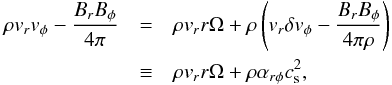 (A.3)and
 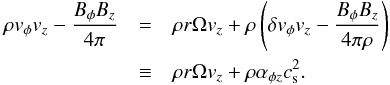 (A.4)We integrate Eq. (A.1) along the vertical direction, z, with Eqs. (A.3) and (A.4) from the bottom surface to the top surface of a disc, and we have
 ![\appendix \setcounter{section}{1} \begin{eqnarray*} \frac{\partial}{\partial t}(\Sigma r^3\Omega) + \frac{\partial}{\partial r} \left[r^2\Sigma \left(v_r r\Omega + \overline{\alpha_{r\phi}}c_{\rm s}^2\right)\right] \end{eqnarray*}](/articles/aa/full_html/2016/12/aa28955-16/aa28955-16-eq255.png)
![\appendix \setcounter{section}{1} \begin{equation} \qquad\qquad +r^2 \left[(\rho v_z)_{\rm w}r\Omega + \overline{\alpha_{\phi z}} (\rho c_{\rm s}^2)_{\rm mid}\right]= 0, \label{eq:amintgz} \end{equation}](/articles/aa/full_html/2016/12/aa28955-16/aa28955-16-eq256.png) (A.5)where
(A.5)where  is the mass-weighted vertical average. The third term, which represents the angular momentum loss from both surfaces, is derived from
 ![\appendix \setcounter{section}{1} \begin{equation} \left[\rho r \Omega v_z + \rho \alpha_{\phi z}c_{\rm s}^2\right]_{\rm w} =[\rho v_z]_{\rm w} r\Omega + (\rho c_{\rm s}^2)_{\rm mid} \overline{\alpha_{\phi z}}, \end{equation}](/articles/aa/full_html/2016/12/aa28955-16/aa28955-16-eq258.png) (A.6)where the subscript w stands for disc wind. is the angular momentum loss by the φz component of the stress normalized by the density and the sound speed at the midplane, Eq. (8).
(A.6)where the subscript w stands for disc wind. is the angular momentum loss by the φz component of the stress normalized by the density and the sound speed at the midplane, Eq. (8).
The equation of mass conservation is  (A.7)By combining Eq. (A.7) multiplied by r3Ω and Eq. (A.5), we have
  (A.8)which determines the accretion rate,
 ![\appendix \setcounter{section}{1} \begin{equation} r\Sigma v_r = - \frac{2}{r\Omega} \left[\frac{\partial}{\partial r} (r^2 \Sigma \overline{\alpha_{r\phi}}c_{\rm s}^2) + r^2\overline{\alpha_{\phi z}}(\rho c_{\rm s}^2)_{\rm mid}\right], \label{eq:accvel} \end{equation}](/articles/aa/full_html/2016/12/aa28955-16/aa28955-16-eq262.png) (A.9)where we here assumed the Keplerian rotation to derive
(A.9)where we here assumed the Keplerian rotation to derive  .
.
By substituting Eq. (A.9) into Eq. (A.7), we finally have the equation for the time evolution of Σ (Eq. (10)): ![\appendix \setcounter{section}{1} \begin{eqnarray*} \frac{\partial \Sigma}{\partial t} - \frac{1}{r}\frac{\partial}{\partial r} \left[\frac{2}{r\Omega}\left\{\frac{\partial}{\partial r}(r^2 \Sigma \overline{\alpha_{r\phi}}c_{\rm s}^2) + r^2 \overline{\alpha_{\phi z}} (\rho c_{\rm s}^2)_{\rm mid} \right\}\right] \end{eqnarray*}](/articles/aa/full_html/2016/12/aa28955-16/aa28955-16-eq264.png)
Appendix B: Energetics of accretion discs
A general MHD expression of the total energy conservation under the axisymmetric approximation is ![\appendix \setcounter{section}{2} \begin{eqnarray*} \frac{\partial}{\partial t}\left[\frac{1}{2}\rho v^2 +\rho \Phi + \frac{p}{\gamma-1} + \frac{B^2}{8\pi}\right] \end{eqnarray*}](/articles/aa/full_html/2016/12/aa28955-16/aa28955-16-eq266.png)
![\appendix \setcounter{section}{2} \begin{eqnarray*} \qquad \left.\left.- \frac{B_r}{4\pi}(v_{\phi}B_{\phi}+v_z B_z)+F_{{\rm ot},r}\right\}\right] \end{eqnarray*}](/articles/aa/full_html/2016/12/aa28955-16/aa28955-16-eq268.png)
![\appendix \setcounter{section}{2} \begin{equation} \qquad \left.- \frac{B_z}{4\pi}(v_r B_r + v_{\phi}B_{\phi}) + F_{{\rm ot},z}\right]= 0, \label{eq:toteng} \end{equation}](/articles/aa/full_html/2016/12/aa28955-16/aa28955-16-eq270.png) (B.1)where we refer to Eq. (11) for the definition of each variable. Decomposing vφ by Eq. (A.2) and assuming
(B.1)where we refer to Eq. (11) for the definition of each variable. Decomposing vφ by Eq. (A.2) and assuming  in a disc, we rewrite Eq. (B.1) with leaving dominant terms. The time-derivative term becomes
 ![\appendix \setcounter{section}{2} \begin{eqnarray*} \frac{\partial}{\partial t}\left[\frac{1}{2}\rho v^2 + \frac{p}{\gamma-1} +\rho \Phi + \frac{B^2}{8\pi}\right] \approx \frac{\partial}{\partial t}\left[\frac{1}{2}\rho v^2 +\rho \Phi\right] \end{eqnarray*}](/articles/aa/full_html/2016/12/aa28955-16/aa28955-16-eq272.png)
![\appendix \setcounter{section}{2} \begin{equation} \qquad \approx \frac{\partial}{\partial t}\left[\frac{1}{2}\rho(r\Omega + \delta v_{\phi})^2 - \rho r^2\Omega^2 \right] \approx \frac{\partial}{\partial t}\left(-\frac{1}{2}\rho r^2\Omega^2\right), \label{eq:tderiv} \end{equation}](/articles/aa/full_html/2016/12/aa28955-16/aa28955-16-eq273.png) (B.2)where we set rΩδvφ = 0 after the azimuthal average. The r-derivative term, except for Fot,r, can be approximated as
(B.2)where we set rΩδvφ = 0 after the azimuthal average. The r-derivative term, except for Fot,r, can be approximated as 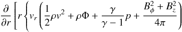
![\appendix \setcounter{section}{2} \begin{eqnarray*} \left.\left.\quad - \frac{B_r}{4\pi}(v_{\phi}B_{\phi}+v_z B_z)\right\}\right] \end{eqnarray*}](/articles/aa/full_html/2016/12/aa28955-16/aa28955-16-eq277.png)
![\appendix \setcounter{section}{2} \begin{eqnarray*} \qquad \approx \frac{\partial}{\partial r}\left[r\left\{v_r\left(\frac{1}{2}\rho v^2 +\rho\Phi\right) - \frac{B_r}{4\pi}v_{\phi}B_{\phi}\right\}\right] \end{eqnarray*}](/articles/aa/full_html/2016/12/aa28955-16/aa28955-16-eq278.png)
![\appendix \setcounter{section}{2} \begin{eqnarray*} \qquad\approx \frac{\partial}{\partial r}\left[r\left\{-\rho v_r \frac{r^2\Omega^2}{2}+\rho r\Omega\left(v_r\delta v_{\phi} -\frac{B_r B_{\phi}}{4\pi\rho}\right)\right\}\right] \end{eqnarray*}](/articles/aa/full_html/2016/12/aa28955-16/aa28955-16-eq279.png)
![\appendix \setcounter{section}{2} \begin{equation} \qquad=\frac{\partial}{\partial r}\left[r\left\{-\rho v_r \frac{r^2\Omega^2}{2}+\rho r\Omega\alpha_{r\phi}c_{\rm s}^2\right\}\right], \label{eq:rderiv} \end{equation}](/articles/aa/full_html/2016/12/aa28955-16/aa28955-16-eq280.png) (B.3)where the second ≈ is derived from
(B.3)where the second ≈ is derived from ![\hbox{$v_r\left(\frac{v^2}{2} + \Phi\right)\approx v_r\left[\frac{(r\Omega+\delta v_{\phi})^2}{2} - r^2\Omega^2\right]\approx - v_r \frac{r^2\Omega^2}{2} + \rho r\Omega v_r \delta v_{\phi}$}](/articles/aa/full_html/2016/12/aa28955-16/aa28955-16-eq281.png) , and for the last equality Eq. (A.3) is used. We set the z-derivative term, except for Fot.z, to be
, and for the last equality Eq. (A.3) is used. We set the z-derivative term, except for Fot.z, to be
![\appendix \setcounter{section}{2} \begin{eqnarray} &&\frac{\partial}{\partial z}\left[v_z\left(\frac{1}{2}\rho v^2 +\rho\Phi + \frac{\gamma}{\gamma -1}p + \frac{B_r^2+B_{\phi}^2}{4\pi} \right) \right. \nonumber\\ &&\left.\qquad - \frac{B_z}{4\pi}(v_r B_r + v_{\phi}B_{\phi})\right] \equiv \frac{\partial}{\partial z}(\rho v_z E_{\rm w}). \label{eq:zderiv} \end{eqnarray}](/articles/aa/full_html/2016/12/aa28955-16/aa28955-16-eq283.png)
In the wind region, the kinetic energy will eventually dominate (Pelletier & Pudritz 1992),  (B.5)provided that the disc wind is accelerated with increasing z.
By substituting Eqs. (B.2)–(B.4) into Eq. (B.1), we obtain
![\appendix \setcounter{section}{2} \begin{eqnarray} && \frac{\partial}{\partial t}\left(-\rho \frac{r^2\Omega^2}{2}\right) +\frac{1}{r}\frac{\partial}{\partial r}\left[r\left\{-\rho v_r \frac{r^2\Omega^2}{2} + \rho r\Omega\alpha_{r\phi} c_{\rm s}^2 + F_{{\rm ot},r} \right\}\right] \\\nonumber &&\qquad+\frac{\partial}{\partial z}(\rho v_z E_{\rm w} + F_{{\rm ot},z})= 0. \label{eq:toteaprx} \end{eqnarray}](/articles/aa/full_html/2016/12/aa28955-16/aa28955-16-eq285.png)
We integrate Eq. (B.7) from the bottom surface to the top surface along z:
![\appendix \setcounter{section}{2} \begin{eqnarray} &&\frac{\partial}{\partial t}\left(-\Sigma \frac{r^2\Omega^2}{2}\right) +\frac{1}{r}\frac{\partial}{\partial r}\left[r\left\{-\Sigma v_r \frac{r^2\Omega^2}{2} + \Sigma r\Omega\overline{\alpha_{r\phi}} c_{\rm s}^2\right\}\right] \nonumber\\ &&\qquad + (\rho v_z)_{\rm w} E_{\rm w}+ F_{\rm rad} =0, \label{eq:totezint1} \end{eqnarray}](/articles/aa/full_html/2016/12/aa28955-16/aa28955-16-eq286.png)
where (ρvz)wEw and Frad are the energy loss by disc winds and radiation from the top and bottom surfaces. Here Frad is from Fot. By substituting Eq. (A.9) into Eq. (B.7), we have
![\appendix \setcounter{section}{2} \begin{eqnarray} &&\frac{\partial}{\partial t}\left(-\Sigma \frac{r^2\Omega^2}{2}\right) +\frac{1}{r}\frac{\partial}{\partial r}\left[r\Omega\left\{ \frac{\partial}{\partial r}(r^2 \Sigma \overline{\alpha_{r\phi}}c_{\rm s}^2) + r^2 \overline{\alpha_{\phi z}} (\rho c_{\rm s}^2)_{\rm mid} \right\}\right. \nonumber\\ && \left. \qquad+ r^2\Omega\Sigma\overline{\alpha_{r\phi}} c_{\rm s}^2\right] + (\rho v_z)_{\rm w} E_{\rm w}+ F_{\rm rad} =0, \label{eq:totezint2} \end{eqnarray}](/articles/aa/full_html/2016/12/aa28955-16/aa28955-16-eq289.png) (B.8)By multiplying Eq. (10) by r2Ω2/ 2, we have
(B.8)By multiplying Eq. (10) by r2Ω2/ 2, we have ![\appendix \setcounter{section}{2} \begin{eqnarray} &&\frac{\partial}{\partial t}\left(\Sigma \frac{r^2\Omega^2}{2}\right) -r^2\Omega^2\frac{\partial}{\partial r} \left[\frac{1}{r\Omega}\left\{\frac{\partial}{\partial r}(r^2 \Sigma \overline{\alpha_{r\phi}}c_{\rm s}^2) + r^2 \overline{\alpha_{\phi z}} (\rho c_{\rm s}^2)_{\rm mid} \right\}\right] \nonumber\\ &&\qquad + (\rho v_z)_{\rm w}\frac{r^2\Omega^2}{2} =0. \label{eq:sgmro2} \end{eqnarray}](/articles/aa/full_html/2016/12/aa28955-16/aa28955-16-eq291.png) (B.9)
(B.9)
By combining Eqs. (B.8) and (B.9), we finally obtain a simple relation for the energetics of disc wind, Eqs. (14) and (15)
![\appendix \setcounter{section}{2} \begin{eqnarray} & & (\rho v_z)_{\rm w}\left(E_{\rm w}+\frac{r^2\Omega^2}{2}\right) + F_{\rm rad} \nonumber\\ &&\qquad =\frac{\Omega}{r}\left[\frac{\partial}{\partial r}(r^2 \Sigma \overline{\alpha_{r\phi}}c_{\rm s}^2) + r^2 \overline{\alpha_{\phi z}}(\rho c_{\rm s}^2)_{\rm mid}\right] -\frac{1}{r}\frac{\partial}{\partial r}(r^2 \Sigma\Omega \overline{\alpha_{r\phi}}c_{\rm s}^2) \nonumber \\ &&\qquad =\frac{3}{2}\Omega\Sigma\overline{\alpha_{r\phi}}c_{\rm s}^2 + r\Omega \overline{\alpha_{\phi z}}(\rho c_{\rm s}^2)_{\rm mid} . \nonumber \end{eqnarray}](/articles/aa/full_html/2016/12/aa28955-16/aa28955-16-eq292.png)
When the disc wind is neglected, (ρvz)w = 0, , Eq. (15) is simplified to  (B.10)where we use Eq. (13). Since the mass accretion rate is approximated as
  , Eq. (B.10) is rewritten as
  (B.11)which is consistent with the expression for the standard accretion disc in the outer region (Shakura & Sunyaev 1973).
All Tables
All Figures
|
Fig. 1 Comparison of time evolutions of four MRI-active PPDs with |
| In the text | |
|
Fig. 2 Comparison of nondimensional mass flux of disc winds, Cw, of the three MRI-active cases except for the no DW case in Table 1. at t = 0 (dotted lines) and 106 yr (solid lines). |
| In the text | |
|
Fig. 3 Mass-loss rate by disc wind, Ṁz, (solid lines) and mass accretion rate induced by the rφ stress, Ṁr,rφ (dashed lines) and by the φz stress, Ṁr,rφ (dotted lines) at t = 106 yr of the four MRI-active cases in Table 1. Ṁz = 0 for the no DW case and Ṁr,φz = 0 for the zero-torque cases. |
| In the text | |
|
Fig. 4 Time evolution of Ṁz (solid) and Ṁr = Ṁr,rφ + Ṁr,φz (dashed) at r = 0.0225 au of the four MRI-active cases in Table 1. |
| In the text | |
|
Fig. 5 Same as Fig. 1 but for four MRI-inactive cases with |
| In the text | |
|
Fig. 7 Comparison of |
| In the text | |
|
Fig. 10 Comparison of normalized pressure gradient force, |
| In the text | |
|
Fig. 11 Migration efficiency for Earth-mass planets for MRI-inactive cases with Σ-dependent torque (red for strong DW and blue for weak DW of Table 2) at t = 106 yr (corresponding to the solid red and blue lines in Fig. 5) in comparison to the MRI-inactive no DW case (black). CI > 0 means outward migration. |
| In the text | |
Current usage metrics show cumulative count of Article Views (full-text article views including HTML views, PDF and ePub downloads, according to the available data) and Abstracts Views on Vision4Press platform.
Data correspond to usage on the plateform after 2015. The current usage metrics is available 48-96 hours after online publication and is updated daily on week days.
Initial download of the metrics may take a while.