| Issue |
A&A
Volume 596, December 2016
|
|
|---|---|---|
| Article Number | A76 | |
| Number of page(s) | 14 | |
| Section | Catalogs and data | |
| DOI | https://doi.org/10.1051/0004-6361/201628531 | |
| Published online | 02 December 2016 | |
Hα-activity and ages for stars in the SARG survey ⋆,⋆⋆
1 INAF−Osservatorio Astronomico di Padova, Vicolo dell’Osservatorio 5, 35122 Padova, Italy
e-mail: This email address is being protected from spambots. You need JavaScript enabled to view it.
2 Dipartimento di Fisica e Astronomia − Universita’ di Padova, Vicolo dell’Osservatorio 3, 35122 Padova, Italy
3 Fundación Galileo Galilei − INAF, Rambla José Ana Fernandez Pérez, 7, 38712 Breña Baja, TF, Spain
4 McDonald Observatory, The University of Texas at Austin, Austin, TX 78712, USA
5 INAF−Osservatorio Astrofisico di Catania, via S. Sofia 78, Catania, Italy
Received: 16 March 2016
Accepted: 23 August 2016
Abstract
Stellar activity influences radial velocity (RV) measurements and can also mimic the presence of orbiting planets. As part of the search for planets around the components of wide binaries performed with the SARG High Resolution Spectrograph at the TNG, it was discovered that HD 200466A shows strong variation in RV that is well correlated with the activity index based on Hα. We used SARG to study the Hα line variations in each component of the binaries and a few bright stars to test the capability of the Hα index of revealing the rotation period or activity cycle. We also analysed the relations between the average activity level and other physical properties of the stars. We finally tried to reveal signals in the RVs that are due to the activity. At least in some cases the variation in the observed RVs is due to the stellar activity. We confirm that Hα can be used as an activity indicator for solar-type stars and as an age indicator for stars younger than 1.5 Gyr.
Key words: binaries: visual / stars: activity / techniques: radial velocities / techniques: spectroscopic
Based on observations made with the Italian Telescopio Nazionale Galileo (TNG) operated on the island of La Palma by the Fundación Galileo Galilei of the INAF (Istituto Nazionale di Astrofisica) at the Spanish Observatorio del Roque de los Muchachos of the Instituto de Astrofísica de Canarias.
A table of the individual Hα measurements is only available at the CDS via anonymous ftp to cdsarc.u-strasbg.fr (130.79.128.5) or via http://cdsarc.u-strasbg.fr/viz-bin/qcat?J/A+A/596/A76
© ESO, 2016
1. Introduction
Studying the variation in the radial velocity (RV) induced by the chromospheric activity is important to distinguish it from the Keplerian motion of the star that may be caused by a planet (see e.g. Queloz et al. 2001; Dumusque et al. 2011; Robertson et al. 2014). On long timescales the active regions can modify measured RVs by introducing a signal related to the stellar activity cycle, while on short timescales the rotational period can become evident.
The most widely used activity indicators are based on the Ca II H&K lines (Isaacson & Fischer 2010; Lovis et al. 2011; Gomes da Silva et al. 2011), which have been shown to correlate with the radial velocity jitter. Other lines were investigated and it was found that the Hα line can be a good alternative (Robinson et al. 1990; Strassmeier et al. 1990; Santos et al. 2010; Gomes da Silva et al. 2011). However the correlation of Hα with Ca II H&K indices is high for the most active stars but decreases at a lower activity level, and sometimes becomes an anti-correlation (Gomes da Silva et al. 2011). Similar results were also found by Cincunegui et al. (2007), who added, using simultaneous observations of stars with spectral type later than F, that the correlation is lost when studying individual spectra of single stars and there is no dependence on activity. The correlation between the averaged fluxes for the Ca II and Hα lines can be clarified by considering the dependence of the two indexes on the stellar colour or the spectral type, while the absence of a general relation between the simultaneous Ca II and Hα index can be due to difference in the formation region of the two lines (Cincunegui et al. 2007; Gomes da Silva et al. 2014). Studying the solar spectrum as a prototype and extrapolating the results to other stars, Meunier & Delfosse (2009) discovered that plages and filaments in the chromosphere contribute differently to Ca II and Hα lines: while plages contribute to the emission of all these lines, the absorption due to filaments is remarkable only for Hα. Therefore the saturation of the plage filling factor seems to enhance the correlation between the two indexes in case of high stellar activity and low filament contribution. On the other hand, the anti-correlation between the emission in Ca II and Hα for low active stars seems to depend only on a strong filament contrast if the filaments are well correlated with plages (see also Gomes da Silva et al. 2014).
A search for planets around the components of wide binaries was performed using the Spettrografo Alta Risoluzione Galileo (SARG) at the Telescopio Nazionale Galileo (TNG) in the past years. Two planetary companions were detected around HD 132563B and HD 106515A (Desidera et al. 2011, 2012). Carolo et al. (2014) found strong variations in the RVs of HD 200466A that could not be explained by a stable planetary system, but which were well correlated to a Hα based activity indicator, showing that they are due to an ~1100-day activity cycle. Stimulated by this finding, we started a systematic analysis of Hα in the binaries of the SARG sample to identify activity-induced RV variations and distinguish them from planetary signatures. We report here on the main results of the activity study made within this survey. We also include the measurements for additional stars observed by our group for other programs carried out with SARG.
2. Observation and data reduction
SARG is the High Resolution Spectrograph at TNG, now decommissioned, which worked for about 12 yr beginning in 2000 (Gratton et al. 2001). The SARG survey was the first planet research program entirely dedicated to binary systems and aimed to determine the frequency of giant planets up to a few AU separation from their star in nearly equal-mass visual binaries using high-precision radial velocities. The sample of the survey included 47 pairs of stars from the Hipparcos Multiple Star Catalog (Perryman et al. 1997), considering binaries in the magnitude range 7.0 < V < 10.0, with magnitude differences between the components ΔV < 1.0, projected separations larger than 2′′ (to avoid strong contamination of the spectra), parallaxes larger than 10 mas, and errors smaller than 5 mas, with B−V > 0.45 mag and spectral types later than F7. For more details on the sample see Desidera et al. (2007). The stars are typically at distance <50 pc from the Sun.
Between September 2000 and April 2012 we collected up to 81 spectra per star with a typical exposure time of 900 s for a total amount of more than 6000 science images.
In this work we also include six bright stars that were observed with SARG looking to search for hot-Neptunes orbiting planets (Gratton et al. 2009). For these stars the integration time was set at 600 s except for 61Cyg B and 40 Eri, for which it was shorter to avoid saturation of the images because of their higher luminosity. τ Cet, 51 Peg and ρ CrB were used as RVs reference stars during the survey, and their signal-to-noise ratio (S/N) is typically greater then 270. In addition, HD 166435 was observed as benchmark active star (Martínez Fiorenzano et al. 2005). We decided to include this star in our sample as well.
Our data set therefore consists of two sub samples: the binary sample and the bright stars sample. The first is unbiased with respect to activity (except for HD 114723, which was excluded because of its high rotation), while the latter has a bias toward low-activity stars except for HD 166435. For all the observations we used the SARG Yellow Grism (spectral range 4600−7900 Å) and the 0.27 arcsec slit to obtain a resolution R = 144 000 with a 2 × 1 pixel binning. The observed spectral range was covered by two chips. The blue chip included the spectral range used for the RV determination: the accuracy was given by a iodine cell superimposing a forest of absorption lines used as reference for the AUSTRAL code (Endl et al. 2000), as shown in Desidera et al. (2011). The red chip data are affected by fringing effects at wavelengths longer than ~7000 Å; these were not used in our analysis. The depth of the iodine lines decreases toward longer wavelengths, and the lines are negligible at the wavelength of Hα.
Data reduction was performed with standard IRAF1 procedures.
3. Stellar parameters
For a proper interpretation of the Hα measurements that we derived in Sect. 4, some stellar parameters were considered. We describe here the adopted sources or procedures to measure them.
Differential radial velocities were derived in Carolo (2012) and have a typical uncertainty of about 4 m/s for stars in the binary survey and less then 2 m/s for the bright stars.
We considered measurements of  from the literature, with preference for studies including multi-epoch measurements to take temporal variations of activity into account. Overall, we retrieved for 36 stars from Wright et al. (2004), Isaacson & Fischer (2010), Desidera et al. (2006b), Strassmeier et al. (2000) and Gray et al. (2003). Finally, for the components of HD 8009, HD 30101, HD 121298, and HD 128041, the value of was derived from HIRES spectra available in the Keck2 archive following the procedure described in Carolo et al. (2014).
For stars without values in the literature we estimated the value from the ratio of X-ray to bolometric luminosity, using the calibration by Mamajek & Hillenbrand (2008). This latter quantity was derived following the procedure described in Carolo et al. (2014) and Carolo (2012) for the sources identified in the ROSAT All Sky Survey (Voges et al. 1999, 2000) within 30′′ from our target stars. For the binaries composing most of our sample, the components are not spatially resolved by ROSAT. We then assumed equal X-ray luminosity for the components. For stars that are not detected in the ROSAT All Sky Survey, this procedure yields an upper limit on . The values of or the upper limits, as other additional parameters we used, are listed in Table A.1.
The projected rotational velocity, vsini, was obtained from a calibration of the full width at half maximum (FWHM) of the cross-correlation function of SARG spectra. Details width be presented elsewhere. For the single stars we adopted the vsini from literature sources such as Valenti & Fischer (2005).
The effective temperature Teff of the primaries was derived from the B−V colour using the calibration by Alonso et al. (1996) and assuming no reddening, while for the secondaries we relied on the high-precision temperature difference measured as part of the differential abundance analysis of 23 binary systems in Desidera et al. (2004, 2006a) and preliminary results by Vassallo (2014) for the others. For the single stars (standard stars and targets of the hot-Neptune program) we adopted the effective temperature from high-quality spectroscopic studies (e.g. Valenti & Fischer 2005).
4. Hα index
Since the Ca II H&K lines wavelengths are not included in the SARG yellow grism spectral range, we defined a new activity index based on the Hα line to study the activity of the stars in this sample. We built an IDL procedure optimized for the SARG spectra format: we measured the instrumental flux (not corrected for the blaze function) in a wavelength interval centred on the line core, FH, and in two additional intervals symmetrically located with respect to the centre, Fc1 and Fc2. Hα is defined as Hα = 2FH/ (Fc1 + Fc2), where Fc1 = flux[6558.80−6559.80 Å], FH = flux[6562.60−6563.05 Å], and Fc2 = flux[6565.20−6566.20 Å]. Since the SARG spectrograph was not built to study in the Hα spectral range, this line appears twice but close to the edges of two orders (close to the blue edge of the order 93 and to the red edge of the order 94), according to the RV of the star. When we choose a wider window for Fc1 and Fc2 or increase the distance from FH, the number of spectra in which the selected wavelength exits the detector therefore increases. Our choice is the best compromise. For the same reason we were unable to use the Hα index that was used by other authors (e.g. Kürster et al. 2003; Boisse et al. 2009; Santos et al. 2010; Gomes da Silva et al. 2014): for each order one of the two continuum reference windows used by these authors is outside of the region covered by the detector. Furthermore, we were unable to use a reference continuum to estimate the continuum flux because it is difficult to define the proper blaze function given the presence of the extended wings of the photospheric Hα absorption. To make our measurement more reliable, we used the weighted mean of two Hα values when fluxes for all these spectral bands could be measured in both orders.
4.1. Error estimation
We then analysed the possible sources of errors.
Internal noise
We estimated the errors on the fluxes assuming photon noise.
The error on Hα index was then derived by error propagation:  (1)where
  , c1err = SNc1/Fc1, c2err = SNc2/Fc2. We note that because of the lower value of the blaze echelle function, the Hα indexes coming from the order 94 have a lower weight on average. HD 128041, HD 143144, HD 9911, 61 CygB and GJ 580A have high absolute radial velocities (RV < −50 km s-1) so that their spectra are remarkably blueshifted. Their Hα indexes have a higher uncertainty because the Hα line is shifted out from the order 93 spectra, therefore we were only able to use the SARG order 94, which yields poorer results.
Systematic error
We also considered that several other sources of noise can introduce errors on the Hα index: flat fielding, background subtraction, bad pixels, instrumental instability, fringing, etc. All these contributions, added to the possible intrinsic variations of activity, increase the standard deviation of the Hα values (σHα). τ Cet was used as a test target for this purpose. It is very bright and its ΔHα variation is lower than 0.005 dex (peak to valley) with low levels of variability in from the literature. We studied the variation of τ Cet night by night. We note that the standard deviation of Hα is about 10 times the intrinsic photonic error, therefore we decided to add a jitter to our measurement. Errors significantly larger than the photon noise error have been reported in other cases of 1 Å wide activity indices from echelle spectra, see for instance Wright et al. (2004). We found that this increase does not depend on the activity level of the star. It is instead described by a relation with the stellar magnitude as shown in Fig. 1:  .
.
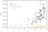 |
Fig. 1 Relation between V magnitude of the stars and the standard deviation σHα of the Hα index. Open symbols indicate quiet stars (see Sect. 4.3 for details), green diamonds are the bright stars sample. The continuous line represents the σjitter we adopted, while the orange asterisks indicate the mean photon noise value for each star. |
Our adopted jitter is compatible with the single night variations of τ Ceti and we rescaled it for other stars according to their magnitude. The dependence on magnitude is that expected for error sources as background subtraction.
Finally the error applied to each measurement of Hα is the sum of the photonic error and the instrumental jitter as derived above. As the jitter is significantly larger then the photon noise, individual errors on Hα index of a given star are very similar. Therefore the estimate of the jitter term has a very limited effect on the periodogram analysis presented in Sect. 6.
Contamination by telluric lines
In the spectral range of Hα we considered, there are several telluric lines mainly due to the water vapour. These lines can enter in our Fc1, Fc2 and FH intervals and influence the Hα index value. The strongest line is H2O at 6564.206 Å. If this telluric line enters FH, the Hα index will decrease of about 1.5%, giving an error by about 0.005 dex on a quiet star. This can occur when the geocentric velocity of the star is between 52 and 75 km s-1. Therefore only a few of our spectra are involved, but none of those discussed below. The effect we have if this line enters Fc2 is about 0.001 dex which is negligible. The H2O line at 6560.555 Å can also enter the FH interval with a comparable contribution if the geocentric radial velocities between − 90 and − 123 km s-1 are involved. These few spectra were rejected.
Contamination estimation
Even though during the observations of the binaries the slit was oriented perpendicularly to the separation of the components, some spectra are strongly contaminated by the companion star and were rejected. Furthermore we modelled the contamination for each consecutive observation of the companions assuming a Moffat-like shape for the point spread function (PSF) and taking into account the separation, the magnitude and the seeing. We obtain that the contribution of the contamination to the Hα is lower then 1% in the majority of the case and therefore is negligible. We found instead that for six systems the variation induced by the contamination is greater than the intrinsic variation (Fig. 2).
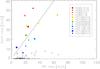 |
Fig. 2 Relation between the standard deviations of the RVs (after the correction for known Keplerian motions) and that induced by the contamination. Systems with a non-negligible contamination are highlighted. |
For example, HD 8071 is a very close binary system (ρ = 2.183′′ according to Hipparcos) and the primary star is a spectroscopic binary with an amplitude of a few km s-1. The effect of contamination on the RV is further modulated by the velocity of the primary at the observing epoch. This causes the RV to vary around the true value by up to a few hundreds m/s in a quite unpredictable way. For more details see Martínez Fiorenzano et al. (2005).
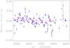 |
Fig. 3 Time evolution of the Hα values of all the spectra normalised to the median value for each star, monthly bins. The red points correspond to the τ Cet data series. |
4.2. Stability of the instrument
The stability of the instrument during the survey was tested: for stars in the binary sample, we normalised the Hα value for each spectrum to the median value of its star. We then binned these values into the synodic monthly mean over different stars and compared them to the same results for the τ Cet data series (see Fig. 3). For τ Cet data we found that points are located around zero with σHα = 0.003. For the stars in the binary sample, the last two years of the campaign were devoted to observing mainly a few stars with candidate companions and/or RV trends, therefore the Hα monthly means depend on the variability of the individual targets, as in the case of HD 200466 (Carolo et al. 2014). We also verified the presence of periodicity by applying the generalize Lomb-Scargle periodogram (GLSP) Zechmeister & Kürster (2009)3 to the two sequences of the binned values: the whole sample sequence shows no significant peak and differs from the τ Ceti sequence, which shows a long-term trend (see Fig. 4).
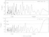 |
Fig. 4 GLSP of the synodic monthly binned Hα values of the SARG sample (top) compared to τ Cet (bottom). |
4.3. Dependence on Teff and ΔHα definition
We divided our sample into two subgroups: as active stars we indicate stars with greater than −4.80, the others are called quiet stars.
Since our Hα index is defined as the ratio between the flux in the line centre and the flux in the wings, we expect that different stars with the same activity level can have different ⟨ Hα ⟩ values because of the different photospheric spectrum. Therefore we compared effective temperature and ⟨ Hα ⟩ to determine the appropriate relation for quiet stars (Fig. 5).
Most of the quiet stars lie at ⟨ Hα ⟩ ~ 0.22 for Teff> 5000 K. At lower temperature, the ⟨ Hα ⟩ index for quiet stars seems to increase. Active stars scatter mostly at higher ⟨ Hα ⟩. We also made a comparison with the Sun: it has an effective temperature of 5780 K and its ⟨ Hα ⟩ is 0.217, as measured in the solar flux atlas (Kurucz et al. 1984), in agreement with the lower envelope for quiet stars. We describe the distribution of the quiet stars in this lower envelope with a three-degree function and define as Hα-excess (ΔHα) the point distance from this line: ΔHα is the difference in Hα index of a star with respect to a quiet star that has the same effective temperature. Therefore we decided to use ΔHα as the activity index; it is more robust than Hα because it allows us to compare the activity of stars with different temperatures.
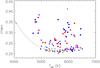 |
Fig. 5 Relation between the temperature and the median value of Hα for each star. Colours are given according to log RHK value sources: values from the literature are plotted in red, while for the blue dots the values are derived from X-ray luminosity. The blue triangles indicate that the |
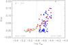 |
Fig. 6 Relation between the |
5. Sample analysis
5.1. Correlation with  and rotation
ΔHα correlates quite well with (reduced χ2 = 2.26, Fig. 6). Active stars are more scattered but typically show excess in the Hα index (ΔHα> 0). All the stars for which has been derived from the X-ray luminosity are in the active portion of the diagram. This is due to the flux limit of the ROSAT All Sky Survey, which is only sensitive to the active stars at the typical distance of our program stars. The stars for which only upper limits are derived populate the lower envelope of the distribution in most cases: this is consistent with a low activity level.
This new index appears to show that stars are distributed in two groups, which suggests the presence of the Vaughan-Preston gap at ΔHα = 0.02 (Vaughan & Preston 1980). The results of Pace et al. (2009) also show the presence of a gap between log RHK = −4.7 and − 5.0. This corresponds to the interval ΔHα ~ [0.01,0.04].
We also found a weak relation between ΔHα and its standard deviation: the intrinsic variation of the Hα index and internal errors contribute to the increase in scatter in the Hα index measurement for each star, but since the scatter is dominated by intrinsic errors for fainter stars, only the deviation seen in brighter stars is dominated by the intrinsic variability.
We also checked the well-known relation between rotation and activity (e.g. Noyes et al. 1984; Baliunas & Vaughan 1985; Santos et al. 2000). We found, as expected, that a moderate rotation is enough to cause a high activity for cold stars and in this case the vsini value increases with activity, while the hottest stars only have high activity values if vsini is high: this behaviour can be related to the decrease in thickness of the convective envelope as the stars become hotter (Charbonneau & Steiner 2012).
5.2. Binary components
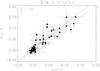 |
Fig. 7 Relation between the ΔHα of the two companion stars. The solid line corresponds to the best fit, the dashed line corresponds to the equivalence. |
We can compare the ΔHα index for the two components in each binary system: we find a very good relation between the two stars indexes, that is ΔHαB = (1.11 ± 0.08)ΔHαA + 0.004 ± 0.004, as shown in Fig. 7. The value of the reduced χ2 suggests that the scatter is dominated by the measurement error. We tested that the long-scale activity cycles (like the solar cycle) induce a variation in Hα that is weaker than our adopted measurement error. HD 108421, HD 132844 and HD 105421 lie above the relation, but we did not note any evidence of errors in our analysis for these stars, so that the discrepancy seems to be real and the two stars of these systems could be in different activity phases. For HD 126246, which lies below the relation, the difference in the Hα activity level between the two components qualitatively agrees with the and vsini difference found by Desidera et al. (2006a), supporting an intrinsic rotation and activity difference between the two components.
5.3. Age-activity relation
Prompted by this result, we tested whether our ΔHα could be an age indicator for these stars (e.g. Skumanich 1972; Baliunas & Vaughan 1985; Soderblom et al. 1993; Mamajek & Hillenbrand 2008; Pace 2013; Zhao et al. 2011). We computed the ages of the binary systems with the isochrone fitting algorithm developed by Bonfanti et al. (2015). The implementations details can be found in Bonfanti et al. (2015, 2016). Here we recall that it enables recovering the isochronal age of a field star when at least its [Fe/H], Teff and log g are available. In our case we also considered as input parameter, which allowed us to disregard unlikely very young isochrones, so that we could better constrain the stellar age. Since the evolution of low-mass stars is extremely slow, this method works well for stars with Teff> 5500 K; for cooler (less massive) stars, uncertainties in the exact location of a star on the Hertzspurng-Russel (HR) diagram leads to an error so large that practically all ages from 0 up to the age of the Universe are possible. We therefore did not consider such stars in our test.
From the differential abundance analysis, Teff and log g have typical uncertainties of ~50 K and ~0.15 dex, respectively, while the differences ΔTeff = TeffA−TeffB and Δlog g = log gA−log gB are more reliable and their reference uncertainties have been estimated in ~20 K and ~0.06 dex, respectively. We therefore constructed a grid in Teff and log g for each binary component, with step sizes of 25 K and 0.05 dex, respectively. We discarded all the points in the grid where the relations ΔTeff−δTeffB< | TeffA−TeffB | < ΔTeff + δTeff and Δlog g−δlog g< | log gA−log gB | < Δlog g + δlog g were not satisfied. We computed the ages of each component for each remaining point in the grid and retained only those for which the stars could be considered coeval (| log tA−log tB | < 0.05; 0.05 is the resolution of the isochrone grids). For each analysed star, we built a catalogue reporting the plausible input parameters and the resulting age that was coeval to that of its companion. For each binary system, we synthesised these data providing the youngest and oldest feasible age of the system and the median age.
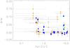 |
Fig. 8 Activity as a function of the age. Blue circles represent the star in Desidera et al. (2004) for which we have solid constraints on the temperature; orange crosses show the other stars. The two systems with an uncertain parallax are highlighted in cyan. |
In Fig. 8 we plot for each star hotter than Teff = 5500 K its ΔHα as a function of the age of the system. We divided the systems into two subsamples according to the reliability of the input parameters, and in particular the Teff: blue dots represent the systems analysed in Desidera et al. (2004), which are more accurate, while orange crosses correspond to preliminary results for systems analysed in Vassallo (2014). The result shows that the majority of the active star are younger than 1.5 Gyr, while for older stars the distribution is flattened around zero, that is, they are inactive.
We found that the activity for young stars is anti-correlated with the age, confirming that the relation between the ΔHα in the components of the systems younger than 1.5 Gyr is mainly due to age. The position of the pairs HD132844A and B and HD 13357A and B in the diagram of Fig. 8 does not follow the general trend: the position on colour-diagram of HD132844 below the main sequence (see Desidera et al. 2004) is indicative of substantial error in the trigonometric parallax. The two Hipparcos solutions for the parallax of HD13357 are inconsistent with each other. In both cases we can conclude that there is an underestimated error in the parallax. Indeed, the adopted parameters (especially the gravity) depend on the adopted trigonometric parallax: in the abundance analysis the effective temperatures were derived from ionization equilibrium and stellar gravities from luminosities, masses and temperatures, using iterative procedures. It seems therefore that a well-defined activity-age relation persists only for objects younger than ~1.5 Gyr, and that after this age Hα seems to be less efficient as an age indicator. Our data did not show significant correlation between these quantities: due to the lack of data with such an age, we cannot conclude whether if there is a discontinuity or if the activity of the star decreases with time. The activity-age anti-correlation for younger stars confirms results from Barry (1988), for example, and the apparent flatness of the plot for older stars seems to agree with Pace (2013); but owing to the uncertainty on our ages, we cannot confirm or reject the idea that the activity decreases with age also for older stars, with a different slope as found by Mamajek & Hillenbrand (2008), for instance. Finally, we found that a large portion (15 over 35) of the stars in our sample with age estimates from the isochrone method are younger than 1.5 Gyr: this could be due to the recent bump in the star formation rate in the solar neighbourhood as claimed by Barry (1988) or to a bias in the age distribution of the stars in the Hipparcos Multiple Stellar Catalog. Future observations of results from the GAIA satellite may clarify this question.
5.4. Activity vs. RV scatter
We finally found the well-known relation between the activity of a star and the standard deviation of its radial velocities (Saar & Donahue 1997; Saar et al. 1998; Santos et al. 2000; Boisse et al. 2009, 2011). In addition, when considering the contamination of the spectra, we found that it is not negligible especially for the systems HD 8071, HD 99121, HD 108421 and HD 209965, which were omitted in this discussion and are detailed below. There are also a number of cases for which the spread in RV during the survey is high (>80 m/s) and which have a relatively low activity level. Most of these objects have known RV trend of Keplerian origin and after the RV variation induced by the companion was removed, they became part of the main trend (Fig. 9). In addition there are at least four stars left outside the general trend. Since these are potentially very interesting objects, we examine them more in detail.
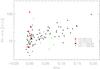 |
Fig. 9 Relation between the ΔHα and the RV standard deviation in the survey. The green dots indicate the RV standard deviation of the stars with a known Keplerian trend that is due to a companion, in red we plot the RV standard deviation of stars with a known companion. In both cases we correct the data for their known RV variation. |
HD 76037A and B: this is a wide binary composed of two F-type stars. The SARG spectra show that the primary star is a long-period partially blended SB2 star, therefore we conclude that the excess scatter in RVs is due to the blending of the spectra of the two components. For the secondary, the excess of the RV scatter is fairly large even after resuming the long-term trend with time that indicates the presence of a low-mass companion; in addition, the Hα index also has a trend with time − more likely related to a cycle.
The Hipparcos Multiple Stellar Catalog indicates that the HD 117963A system has a separation wide enough to rule out contamination effects (ρ = 3.493′′). HD 117963B is a spectroscopic binary and some of the spectra were taken with low S/N (Desidera et al., in prep.). We cannot exclude Keplerian motion as the origin of the scatter for both stars, therefore a deeper analysis with acquisition of additional data would be required.
6. Hα index time-series analysis
By analogy with the Sun, emission in the core of Hα is expected to show time variability mainly modulated by stellar rotation over a period of the order of days, and by the activity cycle over periods of hundreds or thousands of days. In addition, secular variations in the activity levels similar to the Maunder minimum can be present. Therefore the different properties of the time series of our objects should be taken into account. Stars in the hot-Neptunes program were observed for a single season with a moderately dense sampling. In this case rotation periods could be found, but periodicities due to the activity cycle cannot be reliably identified. On the other hand, for the SARG survey objects, the observational campaign was longer and less dense. For only a few targets do we have a larger number of spectra because during the survey they were suspected to host a planet. This was the case of HD 106515A (Desidera et al. 2012) and HD 132563B (Desidera et al. 2011), for example. In addition we already know that for HD 200466A, the RV variations seen are mainly due to an activity cycle (Carolo et al. 2014).
Rank of the Spearman correlation coefficient ρs and its significance between Hα and RV for the stars of the sample.
Stars with cycles.
It is known that more active stars have irregular periods that are not easy to determine with the analysis of periodograms. In spite of this, we computed the GLSPs for the Hα index that was obtained using the Zechmeister & Kürster (2009) procedure. To evaluate the significance of these periodicities, the false alarm probability (FAP) of the highest peak of the periodogram was estimated through a bootstrap method, with 1000 permutations. We used the spectral window function to rule out that our periodicity is due to the sampling. The results for the most interesting objects are listed in Table 2. We found a signature of periodic variations (rotational periods or activity cycles) in 19 stars, whereas 10 stars show a clear overall trend in Hα with time. On the other hand the stars for which we were able to find evidence of activity cycles are all with moderate activity excess and temperatures of between 4800 and 6000 K. The stars showing a long-term trend are hotter than average.
It is noteworthy that of the binary stars that show promising cycles, only HD 76037A and B are quiet and show a long-term trend.
Of the bright stars, 51 Peg was used as a RV standard to monitor instrument performances during the binary program. The quite good temporal coverage of the data allowed us to detect a significant long-term period of about seven years with FAP of 0.6%. Added to this signal, we also found a periodicity of 86.49 d, which corresponds to an alias of the 21.9 ± 0.4 d period found by Simpson et al. (2010) with one sinodic month. This shortest period seems then to be the rotational signal. We obtained a similar result also for 61 Cyg b: the GLSP peaks at 16.44 d, which is an alias of the ~37 d period (Böhm-Vitense 2007; Oláh et al. 2009). 14 Her shows a periodicity of 22.38 d. In this case the spectral window is complex and we cannot rule out that this period is fake. Wright et al. (2004) estimated a rotational period of 48 days from the mean value, but this was not detected by Simpson et al. (2010).
All the Hα time series are available at the CDS.
7. Correlation between RV and Hα
The high uncertainty on the single measurements of Hα prevent us from properly studying the correlation with the RVs. However this was possible in some particular case, such as spectra with high S/N or stars with a relevant trend in Hα. We used the Spearman correlation coefficient ρS and its significance σ to quantify the correlation between RV and Hα index (Table 1): we obtained an extremely high significance for HD 200466A (see Carolo et al. 2014). For four other objects, the probability that the correlation is the result of a random effect is lower than 0.0075. HD 201936A and HD 213013A are active stars with a signature of an activity cycle, GJ 380 spectra have a high S/N and show a probable long-term cycle. Plots are presented in Appendix B. In HD 76037A the anti-correlation simply shows that both RV and activity are time-dependent on long scales. We can therefore rule out a strong physical connection between these two quantities for this star.
8. Conclusions
The activity of 104 stars observed with the SARG spectrograph was studied using an index based on the Hα line. We found that this index, ΔHα, correlates well with the index based on Ca II lines, , and therefore it can be used to estimate the average activity level, confirming previous results. It also correlates with the rotation of the star: low activity corresponds to slow rotation, especially for cool stars. After removing a few targets for which contamination of the spectra by their companion is the dominant source of RV scatter, we found that ΔHα also correlates with the scatter in RV. We obtain that a low-mass companion might be the source of a high residual RV scatter at least for HD 76073B. We also found a strong correlation between the average activity level ⟨ Hα ⟩ of the two components in each binary system and that roughly a half of our systems are active. Finally, we showed that activity as measured by ΔHα is correlated with the age derived from isochrone fitting. Although these have large error bars due to uncertainties in temperature and parallaxes, we found that active stars are typically younger than 1.5 Gyr, while older stars are typically inactive.
We then analysed the time series of the stars: 11 stars (~8.5%) of the SARG sample show a periodicity in Hα with false-alarm probability <0.5%. All these stars have a moderate activity level (0.029 < ΔHα< 0.077) except for the pair HD 76037A and B, but in these cases we only have a hint of a long-term period or magnetic cycle. When we focused on the long-term cycle, we obtained that the temperature interval of these stars is also limited to late-G and early-K stars. Other stars show variabilities on temporal scales certainly different from the rotational periods. In the bright stars sample, we found five stars out of ten with significant periodic variations in Hα. In some cases the physical origin of this type of signal is unclear.
Only five stars show a significant correlation between Hα and RVs.
We conclude that if care is exerted, Hα is a useful indicator for activity and can be a good alternative to Ca II for studies based on radial velocity techniques, especially for solar-type stars.
Acknowledgments
This research has made use of the SIMBAD database, operated at CDS, Strasbourg, France. This research has made use of the Keck Observatory Archive (KOA), which is operated by the W. M. Keck Observatory and the NASA Exoplanet Science Institute (NExScI), under contract with the National Aeronautics and Space Administration. We thank the TNG staff for contributing to the observations and the TNG TAC for the generous allocation of observing time. This work was partially funded by PRIN-INAF 2008 “Environmental effects in the formation and evolution of extrasolar planetary systems”.
References
- Alonso, A., Arribas, S., & Martinez-Roger, C. 1996, A&A, 313, 873 [NASA ADS] [Google Scholar]
- Baliunas, S. L., & Vaughan, A. H. 1985, ARA&A, 23, 379 [NASA ADS] [CrossRef] [Google Scholar]
- Barry, D. C. 1988, ApJ, 334, 436 [NASA ADS] [CrossRef] [Google Scholar]
- Böhm-Vitense, E. 2007, ApJ, 657, 486 [NASA ADS] [CrossRef] [Google Scholar]
- Boisse, I., Moutou, C., Vidal-Madjar, A., et al. 2009, A&A, 495, 959 [NASA ADS] [CrossRef] [EDP Sciences] [Google Scholar]
- Boisse, I., Bouchy, F., Hébrard, G., et al. 2011, A&A, 528, A4 [NASA ADS] [CrossRef] [EDP Sciences] [Google Scholar]
- Bonfanti, A., Ortolani, S., Piotto, G., & Nascimbeni, V. 2015, A&A, 575, A18 [NASA ADS] [CrossRef] [EDP Sciences] [Google Scholar]
- Bonfanti, A., Ortolani, S., & Nascimbeni, V. 2016, A&A, 585, A5 [NASA ADS] [CrossRef] [EDP Sciences] [Google Scholar]
- Carolo, E. 2012, Ph.D. Thesis, University of Padua, Italy [Google Scholar]
- Carolo, E., Desidera, S., Gratton, R., et al. 2014, A&A, 567, A48 [NASA ADS] [CrossRef] [EDP Sciences] [Google Scholar]
- Charbonneau, P., & Steiner, O. 2012, Solar and Stellar Dynamos: Saas-Fee Advanced Course 39, Swiss Society for Astrophysics and Astronomy (Heidelberg, Berlin: Springer) [Google Scholar]
- Cincunegui, C., Díaz, R. F., & Mauas, P. J. D. 2007, A&A, 469, 309 [NASA ADS] [CrossRef] [EDP Sciences] [Google Scholar]
- Desidera, S., Gratton, R. G., Scuderi, S., et al. 2004, A&A, 420, 683 [NASA ADS] [CrossRef] [EDP Sciences] [Google Scholar]
- Desidera, S., Gratton, R. G., Lucatello, S., & Claudi, R. U. 2006a, A&A, 454, 581 [NASA ADS] [CrossRef] [EDP Sciences] [Google Scholar]
- Desidera, S., Gratton, R. G., Lucatello, S., Claudi, R. U., & Dall, T. H. 2006b, A&A, 454, 553 [NASA ADS] [CrossRef] [EDP Sciences] [Google Scholar]
- Desidera, S., Gratton, R., Endl, M., et al. 2007, ArXiv e-prints [arXiv:0705.3141] [Google Scholar]
- Desidera, S., Carolo, E., Gratton, R., et al. 2011, A&A, 533, A90 [NASA ADS] [CrossRef] [EDP Sciences] [Google Scholar]
- Desidera, S., Gratton, R., Carolo, E., et al. 2012, A&A, 546, A108 [NASA ADS] [CrossRef] [EDP Sciences] [Google Scholar]
- Dumusque, X., Lovis, C., Ségransan, D., et al. 2011, A&A, 535, A55 [NASA ADS] [CrossRef] [EDP Sciences] [Google Scholar]
- Endl, M., Kürster, M., & Els, S. 2000, A&A, 362, 585 [Google Scholar]
- Gomes da Silva, J., Santos, N. C., Bonfils, X., et al. 2011, A&A, 534, A30 [NASA ADS] [CrossRef] [EDP Sciences] [Google Scholar]
- Gomes da Silva, J., Santos, N. C., Boisse, I., Dumusque, X., & Lovis, C. 2014, A&A, 566, A66 [NASA ADS] [CrossRef] [EDP Sciences] [Google Scholar]
- Gratton, R. G., Bonanno, G., Bruno, P., et al. 2001, Exp. Astron., 12, 107 [NASA ADS] [CrossRef] [Google Scholar]
- Gratton, R., Desidera, S., & Claudi, R. 2009, MSAIt, 80, 312 [NASA ADS] [Google Scholar]
- Gray, R. O., Corbally, C. J., Garrison, R. F., McFadden, M. T., & Robinson, P. E. 2003, AJ, 126, 2048 [NASA ADS] [CrossRef] [Google Scholar]
- Isaacson, H., & Fischer, D. 2010, ApJ, 725, 875 [NASA ADS] [CrossRef] [Google Scholar]
- Kürster, M., Endl, M., Rouesnel, F., et al. 2003, A&A, 403, 1077 [NASA ADS] [CrossRef] [EDP Sciences] [Google Scholar]
- Kurucz, R. L., Furenlid, I., Brault, J., & Testerman, L. 1984, Solar flux atlas from 296 to 1300 nm [Google Scholar]
- Lovis, C., Dumusque, X., Santos, N. C., et al. 2011, ArXiv e-prints [arXiv:1107.5325] [Google Scholar]
- Mamajek, E. E., & Hillenbrand, L. A. 2008, ApJ, 687, 1264 [NASA ADS] [CrossRef] [Google Scholar]
- Martínez Fiorenzano, A. F., Gratton, R. G., Desidera, S., Cosentino, R., & Endl, M. 2005, A&A, 442, 775 [NASA ADS] [CrossRef] [EDP Sciences] [Google Scholar]
- Meunier, N., & Delfosse, X. 2009, A&A, 501, 1103 [NASA ADS] [CrossRef] [EDP Sciences] [Google Scholar]
- Noyes, R. W., Hartmann, L. W., Baliunas, S. L., Duncan, D. K., & Vaughan, A. H. 1984, ApJ, 279, 763 [NASA ADS] [CrossRef] [Google Scholar]
- Oláh, K., Kolláth, Z., Granzer, T., et al. 2009, A&A, 501, 703 [NASA ADS] [CrossRef] [EDP Sciences] [Google Scholar]
- Pace, G. 2013, A&A, 551, L8 [NASA ADS] [CrossRef] [EDP Sciences] [Google Scholar]
- Pace, G., Melendez, J., Pasquini, L., et al. 2009, A&A, 499, L9 [NASA ADS] [CrossRef] [EDP Sciences] [Google Scholar]
- Perryman, M. A. C., Lindegren, L., Kovalevsky, J., et al. 1997, A&A, 323, L49 [NASA ADS] [Google Scholar]
- Queloz, D., Henry, G. W., Sivan, J. P., et al. 2001, A&A, 379, 279 [NASA ADS] [CrossRef] [EDP Sciences] [Google Scholar]
- Robertson, P., Mahadevan, S., Endl, M., & Roy, A. 2014, Science, 345, 440 [NASA ADS] [CrossRef] [Google Scholar]
- Robinson, R. D., Cram, L. E., & Giampapa, M. S. 1990, ApJS, 74, 891 [NASA ADS] [CrossRef] [Google Scholar]
- Saar, S. H., & Donahue, R. A. 1997, ApJ, 485, 319 [NASA ADS] [CrossRef] [Google Scholar]
- Saar, S. H., Butler, R. P., & Marcy, G. W. 1998, ApJ, 498, L153 [Google Scholar]
- Santos, N. C., Mayor, M., Naef, D., et al. 2000, A&A, 361, 265 [NASA ADS] [Google Scholar]
- Santos, N. C., Gomes da Silva, J., Lovis, C., & Melo, C. 2010, A&A, 511, A54 [NASA ADS] [CrossRef] [EDP Sciences] [Google Scholar]
- Simpson, E. K., Baliunas, S. L., Henry, G. W., & Watson, C. A. 2010, MNRAS, 408, 1666 [NASA ADS] [CrossRef] [Google Scholar]
- Skumanich, A. 1972, ApJ, 171, 565 [NASA ADS] [CrossRef] [Google Scholar]
- Soderblom, D. R., Stauffer, J. R., Hudon, J. D., & Jones, B. F. 1993, ApJS, 85, 315 [NASA ADS] [CrossRef] [Google Scholar]
- Strassmeier, K. G., Fekel, F. C., Bopp, B. W., Dempsey, R. C., & Henry, G. W. 1990, ApJS, 72, 191 [NASA ADS] [CrossRef] [Google Scholar]
- Strassmeier, K., Washuettl, A., Granzer, T., Scheck, M., & Weber, M. 2000, A&AS, 142, 275 [NASA ADS] [CrossRef] [EDP Sciences] [Google Scholar]
- Tody, D. 1993, in Astronomical Data Analysis Software and Systems II, eds. R. J. Hanisch, R. J. V. Brissenden, & J. Barnes, ASP Conf. Ser., 52, 173 [Google Scholar]
- Valenti, J. A., & Fischer, D. A. 2005, ApJS, 159, 141 [NASA ADS] [CrossRef] [MathSciNet] [Google Scholar]
- Vassallo, D. 2014, Master’s Thesis, Universita’ degli Studi di Bologna, Italy [Google Scholar]
- Vaughan, A. H., & Preston, G. W. 1980, PASP, 92, 385 [NASA ADS] [CrossRef] [Google Scholar]
- Voges, W., Aschenbach, B., Boller, T., et al. 1999, A&A, 349, 389 [NASA ADS] [Google Scholar]
- Voges, W., Aschenbach, B., Boller, T., et al. 2000, IAU Circ., 7432, 1 [NASA ADS] [Google Scholar]
- Wright, J. T., Marcy, G. W., Butler, R. P., & Vogt, S. S. 2004, ApJS, 152, 261 [NASA ADS] [CrossRef] [Google Scholar]
- Zechmeister, M., & Kürster, M. 2009, A&A, 496, 577 [NASA ADS] [CrossRef] [EDP Sciences] [Google Scholar]
- Zhao, J. K., Oswalt, T. D., Rudkin, M., Zhao, G., & Chen, Y. Q. 2011, AJ, 141, 107 [NASA ADS] [CrossRef] [Google Scholar]
Appendix A: Additional tables
Stellar parameters.
SARG data.
Appendix B: Stars with RV-Hα correlation
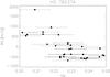 |
Fig. B.1 RV as a function of the Hα index for HD 76037A. |
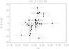 |
Fig. B.2 RV as a function of the Hα index for HD 213013A. |
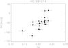 |
Fig. B.3 Decontaminated RV as a function of the Hα index for HD 99121A. |
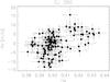 |
Fig. B.4 RV as a function of the Hα index for GJ 380. |
All Tables
Rank of the Spearman correlation coefficient ρs and its significance between Hα and RV for the stars of the sample.
All Figures
|
Fig. 1 Relation between V magnitude of the stars and the standard deviation σHα of the Hα index. Open symbols indicate quiet stars (see Sect. 4.3 for details), green diamonds are the bright stars sample. The continuous line represents the σjitter we adopted, while the orange asterisks indicate the mean photon noise value for each star. |
| In the text | |
|
Fig. 2 Relation between the standard deviations of the RVs (after the correction for known Keplerian motions) and that induced by the contamination. Systems with a non-negligible contamination are highlighted. |
| In the text | |
|
Fig. 3 Time evolution of the Hα values of all the spectra normalised to the median value for each star, monthly bins. The red points correspond to the τ Cet data series. |
| In the text | |
|
Fig. 4 GLSP of the synodic monthly binned Hα values of the SARG sample (top) compared to τ Cet (bottom). |
| In the text | |
|
Fig. 5 Relation between the temperature and the median value of Hα for each star. Colours are given according to log RHK value sources: values from the literature are plotted in red, while for the blue dots the values are derived from X-ray luminosity. The blue triangles indicate that the |
| In the text | |
|
Fig. 6 Relation between the |
| In the text | |
|
Fig. 7 Relation between the ΔHα of the two companion stars. The solid line corresponds to the best fit, the dashed line corresponds to the equivalence. |
| In the text | |
|
Fig. 8 Activity as a function of the age. Blue circles represent the star in Desidera et al. (2004) for which we have solid constraints on the temperature; orange crosses show the other stars. The two systems with an uncertain parallax are highlighted in cyan. |
| In the text | |
|
Fig. 9 Relation between the ΔHα and the RV standard deviation in the survey. The green dots indicate the RV standard deviation of the stars with a known Keplerian trend that is due to a companion, in red we plot the RV standard deviation of stars with a known companion. In both cases we correct the data for their known RV variation. |
| In the text | |
|
Fig. B.1 RV as a function of the Hα index for HD 76037A. |
| In the text | |
|
Fig. B.2 RV as a function of the Hα index for HD 213013A. |
| In the text | |
|
Fig. B.3 Decontaminated RV as a function of the Hα index for HD 99121A. |
| In the text | |
|
Fig. B.4 RV as a function of the Hα index for GJ 380. |
| In the text | |
Current usage metrics show cumulative count of Article Views (full-text article views including HTML views, PDF and ePub downloads, according to the available data) and Abstracts Views on Vision4Press platform.
Data correspond to usage on the plateform after 2015. The current usage metrics is available 48-96 hours after online publication and is updated daily on week days.
Initial download of the metrics may take a while.