| Issue |
A&A
Volume 596, December 2016
|
|
|---|---|---|
| Article Number | A62 | |
| Number of page(s) | 11 | |
| Section | Numerical methods and codes | |
| DOI | https://doi.org/10.1051/0004-6361/201628476 | |
| Published online | 01 December 2016 | |
Stellar longitudinal magnetic field determination through multi-Zeeman signatures
1 Instituto de Astronomia – Universidad Nacional Autonoma de Mexico, Apdo. Postal 70-264, 04510 D.F. México, Mexico
e-mail: This email address is being protected from spambots. You need JavaScript enabled to view it.
2 Armagh Observatory, College Hill, Armagh BT61 9DG, UK
3 Universidad de Guadalajara, Av. Vallarta 2602, Arcos Vallarta, 44100 Guadalajara, Jalisco, Mexico
4 Instituto de Astronomia – Universidad Nacional Autonoma de Mexico, Apdo. Postal 877, 22860 Ensenada, B. C., Mexico
Received: 10 March 2016
Accepted: 7 October 2016
Abstract
Context. A lot of effort has been put into the detection and determination of stellar magnetic fields using the spectral signal obtained from the combination of hundreds or thousands of individual lines, an approach known as a multi-line analysis. So far, however, most of the developed multi-line techniques that retrieve mean stellar longitudinal magnetic fields can sometimes entail substantial simplifications concerning line shapes and Zeeman splittings.
Aims. In this paper we determine stellar longitudinal magnetic fields by means of the Principal Components Analysis and Zeeman Doppler Imaging (PCA-ZDI) multi-line technique, based on accurate polarised spectral line synthesis.
Methods. In this paper we present the methodology for performing inversions of profiles obtained using PCA-ZDI.
Results. Inversions with various magnetic geometries, field strengths and rotational velocities show that we can correctly determine the effective longitudinal magnetic field in stars using the PCA-ZDI method.
Key words: line: profiles / stars: magnetic field / polarization / radiative transfer
© ESO, 2016
1. Introduction
It is well known that magnetic solar-type stars host weak longitudinal fields, typically of the order of a few tens of Gauss (e.g. Marsden et al. 2014). For such field strengths, Stokes V circular polarisation signatures of individual spectral lines are generally well below the noise level. The use of so-called multi-line techniques makes it possible to overcome this problem through the addition of multiple individual lines in Doppler space, resulting in a mean circular polarisation profile, the so-called multi-Zeeman-signature (MZS), which greatly increases the signal to noise ratio. Over the two decades following the pioneering work of Semel & Li (1996) different techniques were developed for the establishment of MZS. The most popular appears to be the least squares deconvolution (LSD) technique first described in Donati et al. (1997). Two assumptions underlie the LSD technique. The first one states that the local circular polarisation profiles to be added are all of similar shape while the second postulates that the Zeeman broadening is very small compared to the thermal Doppler broadening, such that the weak field approximation can safely be applied to the Stokes profiles. As a consequence, the coupled system of equations of polarised radiative transfer do not have to be formally solved. Instead, under a perturbative scheme the system of equations can be partially decoupled, thus permitting one to find an analytical solution: to first order, the circular polarisation profile is proportional to the first derivative of the intensity, and to second order, the linear polarised profiles are proportional to the second derivative of the intensity (e.g. Landi Degl’Innocenti & Landolfi 2004). In recent times, LSD and the weak field approximation (WFA) have been widely employed at different levels of sophistication with the ultimate goal of precisely measuring weak stellar magnetic fields on the basis of MZSs (Kochukhov et al. 2010; Kochukhov 2015; Martínez González & Asensio Ramos 2012; Martínez González et al. 2012; Carroll & Strassmeier 2014; Asensio Ramos & Petit 2015).
An alternative technique based on the principal components analysis (PCA) was proposed by Martínez González et al. (2008). In that study, the MZS is derived by means of the addition of many lines in Doppler space (as in LSD) but a denoising procedure, the filtering of uncorrelated noise, is applied to individual lines to increase the signal to noise ratio in the final MZS. It is an important feature of this technique that similarity between the individual polarised circular line profiles is not required; neither is it necessary to invoke the WFA. The validity of this robust technique for the analysis of magnetic fields has been proven with numerical simulations but the method has not yet been applied to the quantitative measurement of field strengths.
In fact, most current techniques devoted to the analysis of stellar magnetic fields by means of MZS are avoiding spectral line synthesis on account of the computing resources required in view of the wide spectral ranges involved (thousands of Ångströms). To contribute to remedying this situation, we present the basis of a novel technique for the determination of stellar longitudinal magnetic fields, a method that is based on spectral line synthesis incorporating detailed polarised radiative transfer.
2. Solar and stellar Stokes profiles
In this section we use the Stokes profiles obtained from a given single point on the surface of the star − we refer to them here as solar profiles − to derive the Stokes profiles integrated over the entire visible hemisphere of the star; we shall in what follows refer to the latter as stellar profiles. To start with, we first consider a star with zero rotational velocity, but later on this constraint is removed.
A number of parameters must be specified for the calculation of Stokes profiles of magnetic stars. In the present case, we employ the eccentric dipole oblique rotator model (Stift 1975), using the effective temperature Teff, the surface gravity log g, the metallicity [M/H], the projected rotational velocity of the star v sini, the macro-turbulent (vturb) and the micro-turbulent (ξ) velocities, the position of the magnetic dipole inside the star given by the two coordinates x2 and x3, and the dipole moment m. In addition, it is necessary to specify the orientation of the magnetic axis with respect to the rotation axis with the help of the three Eulerian angles α,β and γ, and the orientation of the rotational axis with respect to the line of sight (LOS), that is, the inclination angle i. See Stift (1975) for details. For the synthesis of the Stokes spectra we employed Cossam (Stift 2000; Stift et al. 2012), a local thermodynamic equilibrium (LTE) code that calculates the four Stokes parameters by detailed opacity sampling and by accurately solving the coupled equations of polarised radiative transfer.
2.1. Spatial grids
The so-called effective magnetic field Heff, which represents a weighted average of the longitudinal component of the magnetic field vector over the visible hemisphere of the star, depends on the wavelength range covered by the spectral lines, on their atomic properties, on their strength, and on the limb darkening (Stift 1986). The spatial distribution over the stellar surface of the quadrature points may also play a role if the spatial resolution is too low in the presence of rotation, pulsation and/or strong magnetic fields. Therefore one has to ensure the establishment of a spatial grid containing an appropriate number of well-distributed points. We distinguish two main types of grids; viz. fixed grids and adaptive grids. The Cossam code provides both grid types. Fixed grids can be co-rotating, as found in Doppler mapping (see e.g. Vogt et al. 1987), or be observer-centred. For the former, one tries to create surface elements of almost identical size in bands equidistant in latitude, whereas for the latter the points are arranged in concentric rings about the centre of the visible stellar disk. The concentric rings are very popular because even a relatively small number of such rings usually proves sufficient for the spatial integration required to obtain quantities such as the mean longitudinal magnetic field Heff or the mean field modulus Hs.
Polarised line synthesis in fast rotating stars can constitute a challenge for these simple fixed grids, which may lead to an uncomfortably large number of points. Adaptive grids are better in general, representing non-uniform distributions with no pre-determined distances between the individual points. The central idea behind adaptive grids in line synthesis is that they ensure that the difference in monochromatic line opacity between two adjacent points does not exceed a certain percentage (see Stift 1985, for details). Let us, for example, consider the sampling of the central opacity of a line at a given point. If the grid resolution is not adequately high, at a neighbouring point the line opacity may be negligible as a result of differences in the magnetic field strength and angle, or of the Doppler effect due to rotation or pulsation. The integrated line intensity would thus reach its minimum at one point, whereas at the neighbouring point there would be nothing but the continuum. However sophisticated the quadrature scheme, the integrated line profile would always be in error for such a sparse grid.
In Cossam, the density of points can be adjusted through five parameters. As a proxy for the limit in the relative percentage change in opacity between neighbouring quadrature points one takes a fraction of the Doppler width of the opacity profile of a typical metal line (Rdop). In the polarised radiative radiation equations (see Alecian & Stift 2004) two angles enter: the angle between magnetic field vector and the line of sight (LOS) on the one hand, and the azimuth angle defining Stokes Q and U on the other hand; they are dealt with by Rcos and Razi, respectively. There remains the continuum intensity Rflux, which may not be neglected in the establishment of the spatial grid. Finally, one must ensure the monotonicity of the resolution function in those cases where the Doppler shift between adjacent points is zero and where the field angles are identical. For this purpose, a small empirical constant Δ is added to the resolution function. Adaptive grids are very useful thanks to the optimal placement of the quadrature points and their reduced number compared to fixed grids. This can significantly reduce the time needed to calculate Stokes profiles in strongly magnetic and/or non-radially pulsating stars (Fensl 1995).
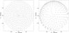 |
Fig. 1 Examples of quadrature point distributions for a rigid (left) and an adaptive grid (right). For illustrative purposes, the number of quadrature points is approximately the same in both cases. |
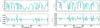 |
Fig. 2 Comparison between solar and stellar (integrated) Stokes profiles. The dashed black line represents the integrated Stokes profiles while the solid line in light colour represents the solar case. The difference in the profiles, shown at the bottom, has been shifted for clarity. The effective longitudinal field strengths are 7.65 G (left panel) and 5.78 G (right panel). |
2.2. Stellar (integrated) versus solar (point source) profiles
We adopted two particular magnetic field configurations and spatial grids for the demonstration of how well stellar Stokes profiles are approximated by solar profiles. In the first case, we assumed an oblique rotator seen equator-on, with the magnetic dipole located at the centre of the star and its axis perpendicular to the rotational axis (Model 1 in Table 1). At phase zero, the magnetic pole is at the centre of the visible disk and the field is thus symmetric around the line of sight. In this case, we employed a fixed grid with ten rings, where the innermost one features eight surface elements, for a total of 440 points, shown in the left panel of Fig. 1. For the second magnetic configuration, labelled Model 2 in Table 1, we chose a decentred tilted dipole, resulting in a highly inhomogeneous distribution of field strengths and angles over the visible hemisphere. With the adaptive grid parameters Δ = 0.5, Rdop = 0.5, Rcos = 0.3, Razi = 0.3, and Rflux = 0.3 we arrived at a total of 406 points distributed as shown in the right panel of Fig. 1.
Magnetic models used for the calculations of the Stokes profiles.
Using Cossam to synthesise the Stokes profiles, from the Atlas9 grid (Castelli & Kurucz 2004) we selected an atmospheric model with Teff = 5500 K, log g = 4.0, solar metallicity, zero macro-turbulence (vturb = 0.0), and a micro-turbulent velocity of ξ = 2.0 km s-1. We then adopted the same dipole moment (m = 10 G) for both models, giving an effective longitudinal field Heff of 7.65 and 5.78 G respectively (for the wavelength range from 4000 to 4050 Å; we note that Heff depends on the wavelength range considered). We also calculated Stokes profiles for the solar case, having the magnetic field vector at the centre of the visible disk pointing towards the observer and setting the value of the field strength equal to the value of Heff. In order to compare the solar to the stellar (integrated) Stokes profiles, we finally normalised them to the continuum.
In what follows, we only discuss the Stokes profiles in intensity I and in circular polarisation V given that in this study we are solely interested in the determination of the longitudinal magnetic field. In Fig. 2 we show the stellar (integrated) Stokes profiles over a narrow interval of 5 Å and the respective solar Stokes profiles. The difference between the stellar and the solar profiles is shown at the bottom of each panel. The Stokes profiles in the left side panels were calculated with the grid shown in the left side panel of Fig. 1; the same applies for the panels on the right-hand side of both figures.
From straightforward visual inspection it is clear that the solar profiles very closely reproduce the Stokes profiles obtained by integration of the local profiles over the visible hemisphere (there are more than 400 points for the two spatial grids). We quantify this result by evaluating the mean absolute error (MAE) of the difference between the solar and the stellar V profiles (lower panels of Fig. 2). Additionally, in order to test how well the effective longitudinal magnetic field can be approximated, we repeat the same procedure for the solar profiles but with increments of ±0.5 G in field strength. The results are listed in Table 2.
We note that, for both grids, the solar fit to the stellar V Stokes profiles is highly accurate. Using the value of Heff for input in a solar-type polarised line synthesis, one obtains a near perfect fit; even a difference of a mere ±0.5 G already leads to a less satisfactory result.
2.3. Including stellar rotation
In the preceding section we showed that solar profiles can be used instead of stellar (integrated) profiles for the analysis of stellar magnetic fields in the case of negligible rotational broadening. In this section we discuss what happens if we include the effects of rotational broadening.
In order to establish a proper broadening function (BF) that can be applied to the solar profiles Sp, producing a correct fit to the stellar rotationally broadened profiles Srot, one has to solve the equation 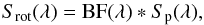 (1)where ∗ denotes the convolution of the two functions and S represents any of the Stokes IQUV parameters. One of two approaches can be used to obtain the BF; viz. the cross-correlation (CC) or the Fourier deconvolution method. The former produces a BF that acts more like a proxy, while the latter provides a more accurate broadening function. Rucinski (1999) showed the advantages of using the Fourier deconvolution rather than CC function, but, more importantly, also showed how the deconvolution approach can be transformed into a linear system of equations which in turn can be solved through Singular Value Decomposition (SVD).
Let m be the number of wavelength points of both solar and stellar profiles, and let n be the number of points (window length) of the broadening function. The central idea is to use Sp to construct a matrix  of dimensions (m−n) × n. Each column in matrix is composed of a segment (of length m−n) of the profiles Sp but shifted vertically by one wavelength element. Let
  denote the segment of interest containing the first m−n elements of Sp. The column arrangement is as follows: the last column of is represented by , the penultimate column by shifted by one wavelength element, and so on. Finally, for the proper handling of the edges of the profiles Srot, a reduction from m to m−n elements is applied. This allows for the removal of n/ 2 points from each side of Srot (more details can be found in Rucinski 1992; and Rucinski 1999). By applying this rearrangement, Eq. (1) is transformed to a linear system of equations:
 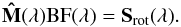 (2)This system of equations is solved by applying SVD to , from which we obtain the orthonormal matrices Û and
  and the vector w, with respective dimensions of (m−n) × n, n × n, and n (see e.g. Golub & van Loan 1996). With the elements of the vector w, it is possible to define the square matrix Ŵ1 (with dimensions n × n) which is only different from zero in the diagonal elements as W1(i,i) = w(i). It is then possible to write the matrix as the product of these three matrices:
  (3)Let us now define Ŵ as the diagonal matrix whose elements are the inverse of the diagonal elements of Ŵ1, viz. W(i,i) = 1 /w(i). Finally, taking the inverse of the orthonormal matrices U and V (their transposes), it becomes possible to recover the broadening function as (omitting the dependence on λ):
  (4)SVD has many interesting properties, one of them being that the eigenvectors in Û and
  are arranged in order of importance. This fact allows a reduction of dimensionality without loss of useful information. In practice, we implement the dimensionality reduction by storing a number l<n of elements in the diagonal of the matrix Ŵ. To illustrate how to find the optimal number l, we use the circular Stokes profiles shown in the right panels of Fig. 2. Let S0 denote the solar Stokes profiles and S10 the stellar (integrated) Stokes profiles calculated with the adaptive grid and v sini = 10 km s-1. We first calculate the Stokes profiles with only one eigenvector (l = 1) using Eq. (1), i.e. S10 = BFl = 1 ∗ S0. Subsequently, we increase l gradually until the full length of the BF is reached (l = n = 301).
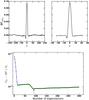 |
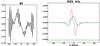
Fig. 3 Upper left panel: a wide broadening function using a spectral window of 301 points. Upper right panel: optimal BF(x) with 91 spectral points. The independent variable x has been substituted for λ in order to emphasise that the sampling rate is at constant velocity steps (1.0 km s-1 in our case). Lower panel: comparison of V Stokes parameters as a function of the number of eigenvectors included in the BF. The optimum fit achieved with 91 eigenvectors is indicated by an arrow. |
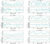 |
Fig. 4 Same as in Fig. 2 but considering different rotation velocities: from top to bottom 5, 10 and 20 km s-1, respectively. |
In Fig. 3 we show the BF using the full length of the spectral window (upper left panel), and the one that gives the best fit (upper right panel). The accuracy of the fits as a function of the number of eigenvectors included while constructing the BF is displayed in the lower panel. Note that the fit of the profiles improves quickly as the number of eigenvectors increases. It then enters a plateau phase, subsequently improving once more until reaching the optimum fit (l = 91), before finally entering a second plateau phase. The explanation for this particular behaviour is twofold. Firstly, the continuum regions do not contain information about the broadening process (e.g. Rucinski 1992), and secondly, the numerical value in these continuum regions is very close to, but not exactly, zero. These two properties mean that the curve shows this two-plateau behaviour. We have corroborated this fact by adding noise to the profiles, and in this case the fits improve monotonically until the optimum fit is reached. Of course, the fit is better when there is no noise. In the noise-free case, the difference between solar and stellar V profiles for the optimum fit is gratifyingly small (MAE of 8.6 × 10⁻⁶), and in fact even better than the fits found for the case of v sini = 0 listed in Table 2. It has to be kept in mind that in real observations, the latest eigenvectors are associated with noise. Hence, it is important to carefully determine the optimum number of eigenvectors to use in the construction of the BF.
We applied the broadening procedure to the Stokes profiles shown in Fig. 2 with values of v sini of 5, 10, and 20 km s-1. It turns out that the adaptive grid is very sensitive to the value of v sini. We have therefore modified the parameters of the adaptive grid in such a way as to obtain a number of points comparable to the one used for the fixed grid (close to 400). The resulting profiles are shown in Fig. 4 and demonstrate that the broadening procedure applied to the solar profiles is working properly. We note that the BF properly reproduces both the broadening due to rotation and the broadening due to the distribution of magnetic field strength across the stellar surface. This becomes even more clear in the following section where higher magnetic field strengths are considered.
3. Multi-line technique
We now want to investigate whether it is possible to generalise our results to spectral ranges of thousands of Ångströms, to strong magnetic fields and to non-zero rotational velocities. For this purpose, in what follows we shall employ the PCA-ZDI multi-line technique developed by Semel et al. (2006). Details concerning the addition properties of individual lines in the context of this technique have been presented in Semel et al. (2009), and a detailed description of the procedure used to obtain the MZSs as well as a discussion of some of their properties are given in Ramírez Vélez et al. (2010). Please note that ZDI is used here in the original sense introduced by Semel (1989), not to be confused with the mapping of magnetic and/or abundance structure, as in Hussain et al. (2000), for example. The PCA-ZDI technique is based on a representative database of synthetic Stokes spectra, calculated in the present study with the help of Cossam; PCA is used to obtain the eigenvectors of that database. Subsequently, these eigenvectors serve as detectors (in analogy to the line mask used in LSD), in order to obtain the MZSs through a cross correlation between the observed spectra and the eigenvectors. In order to prevent confusion, let us emphasise that the eigenvectors used in the PCA-ZDI technique have nothing to do with the eigenvectors used for the construction of the BFs described previously. In fact, the eigenvectors used in PCA-ZDI form the basis of the Stokes parameters in the synthetic database, such that any Stokes profile in that database can be represented by a linear combination of the PCA-ZDI eigenvectors. For more details, see the three references given above.
With the PCA-ZDI technique it is possible to obtain one MZS per eigenvector, that is, as many as the model spectra contained in the database (a total of 700 for this work, see below). However, the first eigenvector is the most significant one, exhibiting the most representative line shape pattern of all models included in the database. Thus, in order to simplify the interpretation of the results, for our tests and analyses we shall employ only the MZS obtained with the first eigenvector.
In addition, given that nowhere in the whole procedure has similarity of the individual lines been assumed nor any special regime of the magnetic field strength and direction, our technique does not suffer any of the constraints typical for LSD. Our only restriction is a minimum ratio of line-depth to continuum, which for this work we have fixed at >0.1, resulting in a total number of individual lines used for the construction of MZSs of approximately 38 000.
The first magnetic detections with the help of PCA-ZDI in linear and circular polarisation were presented a decade ago (Semel et al. 2006; Rámirez Vélez et al. 2006), but magnetic field quantities such as Heff have not yet been determined with this technique. In the following we show how stellar effective longitudinal magnetic fields can be retrieved by application of PCA-ZDI.
3.1. MZS using PCA-ZDI
We have considered a wide spectral range from 350 to 1000 nm in steps of 1 km s-1 (yielding a total of ~315 000 wavelength points). Adopting the same atmospheric model as before, we built a database of Stokes profiles for the solar case, with the magnetic field varying between 0 and 350 G in steps of 0.5 G. From this database we obtained the eigenvectors, but we then used only the first eigenvector to produce a total of 700 solar MZSs. Our goal was to retrieve Heff (a stellar (integrated) quantity) by converting solar MZSs to stellar MZSs, similarly to what we did in the preceding section.
For this purpose, let us consider the stellar MZS obtained from Model 1 of Table 1, v sini = 10 km s-1 and a magnetic moment of m = 400 G. The effective field for this configuration at phase zero is 256 G. We then search in the solar space of MZSs for a model with field strength equal to the value of Heff. Now we are confronted with the same situation as before, that is, we have to apply the appropriate broadening to the solar MZS to reproduce the stellar MZS yet instead of working with spectral lines, viz. Eq. (1), we work with the MZSs:  (5)where MZSrot stands for the stellar MZS, MZSp for the solar MZS and X indicates that we are working in Doppler space.
The broadening function is found as explained in the preceding Sect. 2.3. In the left panel of Fig. 5 we show the optimum BF and in the right panel we show the solar MZS (red line), the stellar MZS (dashed black line), and the solar broadened MZS (full line in cyan). The difference between the last two MZSs is shown at the bottom of the panel (full line in green).
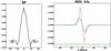 |
Fig. 5 Left panel: optimal BF, derived with 41 eigenvectors. Right panel: MZS profiles. The red line represents the solar MZS (v sini = 0 km s-1), the dashed black line the stellar MZS (v sini = 10 km s-1), and the solid line in cyan the result of the application of the BF to the solar MZS. The green line at the bottom of the panel, shifted for clarity’s sake, represents the difference between the solar broadened MZS and the stellar MZS. The stellar Stokes profiles were calculated using Model 1, a dipolar magnetic moment of m = 400 G and a fixed grid of 440 quadrature points. |
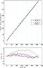 |
Fig. 7 Upper panel: inversion of MZSs using the fixed grid with a centred dipole pointing towards the observer (Model 1 of Table 1). The various values of v sini are shown with different symbols and colours. Lower panel: inversion errors. |
We now want to demonstrate that a BF established this way can be applied irrespective of the strength of the effective longitudinal field Heff. To this end, we simply apply the BF to all solar MZSs and verify whether or not the Heff values for a set of stellar MZSs with different magnetic field strengths can be correctly recovered. Please note that the inversions concern only circular Stokes profiles and do not include the MZSs in intensity. By varying the magnetic moment (m = [5, 10, 20, 30 ... 490 G]), we produce 50 stellar MZSs, carrying out this procedure for the three values of v sini previously used: 5, 10 and 20 km s-1. It has to be emphasised that, for each value of v sini, it is mandatory to find the appropriate BF. The results displayed in Fig. 7 clearly show that our approach leads to the correct retrieval of the stellar Heff.
Nevertheless, it is important to realise that the BF also depends on the orientations of the principal axes of the system; combinations of the three Eulerian angles α, β and γ, and of the inclination angle i between rotation axis and the LOS. To illustrate this dependence, we took the example shown in Fig. 5 and recalculated it, this time using the angles of Model 2 instead of the geometry of Model 1. For this new configuration, the longitudinal field value drops to Heff = 212 G, but much more importantly, the shape of the MZSs and the BF change drastically (see Fig. 6).
We have established that for the recovery of the effective longitudinal field Heff, one cannot use arbitrary BFs. In other words, not only for each rotational velocity, but also for each orientation of the principal axes of the system, there exists a particular associated BF that allows the proper recovery of Heff. To illustrate this fact, we repeated the field inversions of the 50 stellar MZSs calculated with Model 1, but this time, in order to broaden the solar MZSs, we used the BF of Model 2 (left panel of Fig. 6). From the results (not shown) it becomes abundantly clear that the field inversions fail completely. In practice, when dealing with observational data, it is not possible to know a priori the orientation of the principal axes. We thus have to devise a method that generalises the field inversion procedure to any arbitrary orientation.
3.2. Magnetic field inversions for arbitrary orientations
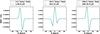 |
Fig. 8 Examples of three stellar MZSs (dashed black lines) and their respective inversions (solid lines in light colour). The values of Heff are well retrieved in all cases as shown in the legends of each panel. Both the solar field strength and Heff are given in Gauss. |
We now want to demonstrate that it is possible to correctly recover the effective longitudinal field from MZSs for arbitrary combinations of the angles α, β and γ, and of the inclination i. Considering v sini = 10 km s-1, adopting a magnetic moment of m = 400 G (not implying any loss of generality) and randomly varying the four angles, we calculated 600 different stellar MZSs at phase zero. For each combination of the angles, we obtained a particular stellar MZS with an attached value of Heff and an associated BF. Each of these 600 BFs were obtained following the same process employed in Figs. 5 and 6, that is, by solving Eq. (5) based on the method described in Sect. 2.3. All the BFs were constructed consistently with the same number of eigenvectors (41). Now let BFn denote the broadening function associated with the nth combination of angles. This BFn was directly applied to the 700 solar MZSs; each one having a different value of field strength from 0 to 350 G in steps of 0.5 G. Repeating this process for all the BFs results in a total of 600 × 700 solar broadened MZSs, all of which are characterised by a particular combination of angles and magnetic field strengths.
Considering the same rotation value of vsini = 10 km s-1, we then calculated a set of 100 stellar MZSs with random variations of the four angles α, β, γ and i, and of the dipolar magnetic moment (between 0 and 490 G). We inverted these stellar MZSs in the database made up of the broadened solar MZSs. Figure 8 shows detailed fits of 3 among the 100 stellar MZSs, suggesting that our proposed technique is able to recover the effective longitudinal field of a star relatively accurately. The results for the whole bulk of 100 stellar MZSs are displayed in Fig. 9 and definitely validate the excellent performance of the method, reflected in gratifyingly small errors.
These encouraging results were obtained, implicitly, only for the special case where the dipole position is known a priori (in our latest example at the centre of the star). More generally, one has, however, to consider all the parameters of the magnetic model to be unknown, a problem which we address in the following section.
3.3. Retrieving Heff in the general case
We performed a similar test to the one presented in the preceding section but this time including the position and direction of the dipole as unknowns. We calculated 7500 stellar MZSs, varying all the parameters in the magnetic model (α, β, γ, i, x2, x3) randomly. The position of the dipole was constrained to less than 0.3 R⋆. The angles (α, β, γ) were allowed to vary between − 180deg and + 180deg, and the inclination i between 0deg and + 180deg. Please note that with these limits to the range of the Eulerian angles, there is a certain redundancy in the resulting models, so that we can fix the rotational phase arbitrarily at zero. Finally, we arbitrarily adopted a magnetic moment of 400 G as before and also assumed a value of vsini = 10 km s-1.
For each of these MZS we repeated the procedure described in the last section, that is, for any given combination of magnetic parameters we obtained an associated MZS with a particular value of Heff and an attached BF. Considering all the calculated magnetic models, we obtained a total of 7500 BFs that we applied to broaden the solar MZSs, reaching a total of 7500 × 700 solar broadened MZSs. Again, each of these solar MZSs is distinguished by a particular combination of magnetic geometry and field strength. Then, to test the inversions, we calculated a set of 100 stellar MZSs adopting v sini = 10 km s-1 and random values of the four angles, of the dipole moment (between 0 and 690 G) and of the dipole position (<0.3 R⋆). We show the results of the inversions in Fig. 10.
These plots reveal that none of the geometric model parameters (α, β, γ, i, x2, x3) can be correctly retrieved. This is not surprising since, for a given value of Heff, a multiplicity of combinations of angles, magnetic moments and dipole positions can produce the same stellar longitudinal field. Nevertheless the value of Heff is, in general, well-retrieved. The inversion errors for Heff are larger than in the case of a fixed dipole position. Furthermore, in our tests we have considered the atmospheric model (Teff, log g, [M/H], vturb, ξ) as fixed and for this reason we have not included Stokes I in the inversions; when inverting simultaneously the Stokes I and V parameters, in the case of real data, the inversion incertitudes will increase. However, please note that a way to reduce the inversions errors is to increase the number of BFs considered (7500 in this test). We thus may conclude that it is possible with our method to correctly measure stellar longitudinal magnetic fields.
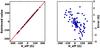 |
Fig. 9 Recovery of Heff from stellar MZSs (at left) and uncertainties (at right), considering α, β, γ, i, and the magnetic moment m as variable parameters. The MZSs were calculated using an adaptive grid (~80 points). |
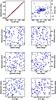 |
Fig. 10 Inversion of stellar MZSs in general, using a fixed grid (80 points) and considering all the parameters in the magnetic model (α, β, γ, i, x2, x3, m) as unknowns. In each panel the x axis gives the values of the input parameters to the stellar MZS. The y axis of the upper right panel gives the inversion errors for the Heff, for the rest of the panels it gives the parameter values retrieved by the inversions. |
3.4. Spatial grid resolution with PCA-ZDI profiles
Throughout this work we have used both adaptive and fixed grids at different spatial resolutions. Now we want to show that the database used in the last test, based on 80 spatial quadrature points, can be used to invert MZSs calculated at much higher spatial grid resolution (up to 1000 points and more). For this purpose we have considered two arbitrary magnetic models whose parameters are listed in Table 3. Taking an adaptive grid with 80 quadrature points and a magnetic moment of 39.26 G, for Model 1, one obtains Heff = −24.32 G at phase zero. Similarly, adopting a value of m = 395.78 G, we find Heff = 228.90 G at phase 0.526 for Model 2.
As mentioned at the beginning, Heff is a quantity that depends on the limb darkening, being thus potentially affected by the number and the spatial distribution of the quadrature points. We have inspected this problem with the help of the two magnetic models of Table 3, varying the grid resolution. In Fig. 11 we plot Heff as a function of the number of grid points; the values of Heff are given relative to the value of Heff calculated with an 80-point grid. We see a modest but significant change in Heff when the number of grid points is increased to approximately 500, reaching a difference of approximately 4% and 3% for Models 1 and 2, respectively. Further increasing the number of points gives only very small variations in Heff. For Model 1 Heff remains essentially constant when the number of grid points is in excess of 600, whereas for Model 2 the normalised longitudinal field passes from 97.2% to 96.9% between 502 and 1096 grid points. We therefore consider a grid resolution of approximately 1000 points sufficient for highly accurate Heff determinations in both models.
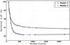 |
Fig. 11 Percentage variation of Heff as a function of the number of quadrature points considered in the adaptive grid. The Heff values are normalised to the Heff value obtained with a grid of 80 points. |
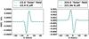 |
Fig. 12 Examples of two stellar MZSs constructed at very high grid resolution (>1000 points) using adaptive grids. The dashed black lines represent the stellar MZSs while the solid lines in cyan colour are their respective inversions. The retrieved values of the Heff (shown at the top of the panels) clearly indicate that the PCA-ZDI profiles are quite insensitive to the grid resolution. |
Magnetic models used to test the spatial grid resolution.
We thus established the stellar MZSs for Models 1 and 2 at high resolutions (1096 and 1146 points, respectively), employing an adaptive grid. We then inverted these two MZSs in the solar broadened database used for the test presented in the preceding section. Please note that the BFs applied to broaden the solar MZSs of that database were obtained from stellar MZSs established with a fixed grid of 80 points. We then performed the same inversions again, but now using a fixed grid of 1100 points to establish the two stellar MZSs. The results shown in Figs. 12 and 13 clearly reveal that we can properly retrieve Heff from the stellar MZSs constructed at high grid resolution.
Let us explain the reasons for this gratifying result. After inspection of the V profiles at different grid resolutions, we found that in general differences in the integrated stellar Stokes profiles are small; the spatial grid resolution can have some influence for only a small number of lines. For Model 1, for example, comparing the adaptive grids at high and low resolution, 1046 and 80 points, respectively, we found a MAE of the V profiles of 4.5 × 10⁻⁵, whereas the maximum difference in the line profiles is 2.3%. Accordingly, when constructing the MZSs through the addition of thousands of lines, the differences in the Stokes profiles cancels out statistically, permitting the correct retrieval of Heff. One would however expect the resolution of the spatial grid to have more important repercussions on the synthesis of Stokes profiles in the presence of very strong magnetic fields, fast stellar rotation or strong stellar pulsations (e.g. Fensl 1995), a case outside the scope of the present study.
To conclude, the results of Figs. 12 and 13 are very encouraging since the most time-consuming part of our method lies in the computation of thousands of stellar MZSs that serve to obtain the BFs that we use to broaden the solar MZSs. The fact that for the calculation of the stellar MZSs we can employ a relatively low spatial grid resolution without compromising the results makes our approach less expensive than might have been feared.
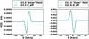 |
Fig. 13 Same as Fig. 12 but considering a fixed grid of 1100 points in the construction of the stellar MZSs. |
4. PCA-ZDI and (magnetic) broadening
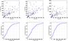 |
Fig. 14 Upper panels, from left to right: mean, minimum and maximum surface values of the field modulus as a function of the absolute value of Heff for the set of 100 MZSs used in the inversion test of Fig. 10. Lower panels: respective cumulative histograms. |
The surface distribution of the local magnetic fields is known due to obtaining the stellar spectra through the integration of the local Stokes profiles. Let us for example have a look at the 100 MZSs employed for the inversion test shown in Fig. 10. Recall that for the establishment of this set of MZSs, all the parameters of the magnetic model were randomly varied. In the upper panels of Fig. 14 we plot the mean, minimum and maximum values of the field modulus as a function of | Heff | for the full set of MZSs. The lower panels display their respective cumulative distributions. Not surprisingly, small absolute values of Heff can be accompanied by large field moduli which means that Heff cannot be taken as an indicator for the validity of the weak-field approximation. In our sample, for example, we encounter a value of Heff = 24.6 G, associated with mean, minimum and maximum values of 1443, 797, and 2120 G respectively. Unlike other multi-line techniques, the PCA-ZDI technique allows us to correctly recover Heff irrespective of the distribution and intensities of the local magnetic fields (see upper panels of Fig. 10).
To summarise, our approach does not require any of the following assumptions:
-
1.
That the local residual Stokes I intensities are small (see e.g. discussion by Sennhauser et al. 2009, and also that by Kochukhov et al. 2010);
-
2.
that the magnetic broadening is largely inferior to the non-magnetic broadening (thermal, rotational, micro/macro turbulence);
-
3.
that the Zeeman splitting results in a normal triplet for all lines.
In other words, with the PCA-ZDI technique we can correctly deal with blended lines, take into account the anomalous Zeeman effect or negative Landé factors for individual lines and work in the presence of strong magnetic fields such that the spectral lines are in the regime of Zeeman saturation, that is, the amplitudes of the V profiles do not grow anymore linearly with the intensity of the magnetic field. This considerably widens the application range of our method compared to other multi-line techniques such as LSD, for example.
In addition, we have verified that the weak field approximation can not be applied to retrieve Heff from the MZSs. We find that the shape of the derivative of the Stokes I MZS does not correspond to the shape of the Stokes V MZS, indicating that PCA-ZDI is incompatible with the WFA. The reason for this is simply that our technique does not require the assumptions of the WFA to be valid.
Finally, we would like to emphasise that the fits to the MZSs (Figs. 8, 12 and 13) clearly indicate that magnetic and rotational broadening are adequately taken into account by the BF method simultaneously.
5. Conclusions
Spectropolarimetry constitutes the optimum observational technique for the study of solar and stellar magnetism. These data are best analysed with the help of codes that implement spectral line synthesis in the presence of magnetic fields, solving the coupled equations of polarised radiative transfer. It is highly desirable that any multi-line approach to the determination of global magnetic quantities, such as the effective longitudinal field Heff or the mean magnetic field modulus Hs, should incorporate full opacity sampling and a correct treatment of polarised radiative transfer when calculating local Stokes IQUV profiles. This is exactly what we have done with the help of a database of Stokes profiles established using the polarised line synthesis code Cossam and MZSs obtained by means of the PCA-ZDI technique.
Efforts to derive Heff from MZSs obtained with PCA-ZDI date back to Semel et al. (2009) who showed that the centre of gravity method can be applied to the MZSs for an estimate of magnetic field strengths. Additionally, using all four Stokes parameters, Ramírez Vélez et al. (2010) demonstrated that MZSs correctly encode the information on the magnetic field, meaning that both strength and orientation of the magnetic field can be successfully recovered for field strengths of up to 10 kG. In these two papers, the results were obtained using solar MZSs, that is, any effect of rotation was neglected and no inhomogeneous spatial distribution of magnetic strengths was assumed over the surface.
The present study introduces a novel approach that can be applied to the analysis of spectropolarimetric data. The principal idea behind this method consists of the use of broadened solar MZSs to infer the effective longitudinal field Heff. We have shown that the BFs are an effective tool to properly reproduce the rotational and magnetic broadening effects on the Stokes profiles in wavelength space, much as they are for the MZSs in Doppler space. We have tested our approach for different moderate values of vsini, obtaining good results in all cases. Gratifyingly it has been found that the results do not depend on whether one uses fixed grids or adaptive grids.
Cossam, the polarised spectral line synthesis code employed in this work, is considered a reference for the calculation of stellar Stokes parameters (Wade et al. 2001; Carroll et al. 2008). For the inversion (in the general case) of the stellar MZSs, we adopted fixed stellar atmospheric model parameters (Teff, log g, [M/H], vturb, ξ), but freely varied the parameters of the magnetic model incorporated in Cossam, viz. the magnetic moment m, the Eulerian angles α, β, and γ, the vector of the dipole offset [0, x2, x3] and the inclination i. We were able to demonstrate that solar broadened MZSs are able to reproduce the shape of stellar MZSs, providing us with the possibility of determining Heff. Currently, Cossam assumes a tilted eccentric dipole, but our technique should also work for quadrupolar or higher-order configurations, even for magnetic fields concentrated in starspots.
Computing times for the (point-source) solar MZSs are of course largely inferior to those for (integrated) stellar MZSs which increase in proportion to the number of spatial quadrature points. Still, for the approach presented here, extensive calculations are required to arrive at the significant number of stellar MZSs needed to establish the BFs that serve to broaden the solar MZSs. A 56 core workstation required approximately three weeks to obtain 7500 stellar MZSs covering the interval from 350 to 1000 nm in steps of 1 km s-1, and adopting an 80 point spatial grid. It might, at this point, be legitimately asked why one should spend such an effort on the determination of Heff instead of trying to directly model the stellar MZSs. Given the huge number of combinations in the parameter space of the tilted eccentric dipole model, an obvious reason for wanting to know the effective longitudinal field at various phases is so that this number can be reduced, possibly by a very large amount. The availability of (even modestly sized) supercomputers can greatly increase the attractiveness of our method. In a forthcoming paper we present the application of this technique to observational data.
Acknowledgments
J.R.V., S.G.N. and L.S. acknowledge support from the CONACyT grants 240441, 168078 and 180817 respectively. Part of the results presented here have been obtained using the “Supercomputo – DGTIC” facilities, grant SC16-1-IR-40, of the UNAM, the computers from the CONACyT project 153985 and the UNAM-PAPIIT project 107215, and the computers “Tychos” (Posgrado en Astrofisica-UNAM, Instituto de Astronomia-UNAM and PNPC-CONACyT). LS also acknowledges support from the grant UNAM-DGAPA-PAPIIT IA101316. Thanks go to AdaCore for providing the GNAT GPL Edition of its Ada compiler.
References
- Alecian, G., & Stift, M. J. 2004, A&A, 416, 703 [NASA ADS] [CrossRef] [EDP Sciences] [Google Scholar]
- AsensioRamos, A., & Petit, P. 2015, A&A, 583, A51 [NASA ADS] [CrossRef] [EDP Sciences] [Google Scholar]
- Carroll, T. A., & Strassmeier, K. G. 2014, A&A, 563, A56 [NASA ADS] [CrossRef] [EDP Sciences] [Google Scholar]
- Carroll, T. A., Kopf, M., & Strassmeier, K. G. 2008, A&A, 488, 781 [NASA ADS] [CrossRef] [EDP Sciences] [Google Scholar]
- Castelli, F., & Kurucz, R. L. 2004, ArXiv e-prints [arXiv:astro-ph/0405087] [Google Scholar]
- Donati, J.-F., Semel, M., Carter, B. D., Rees, D. E., & Collier Cameron, A. 1997, MNRAS, 291, 658 [NASA ADS] [CrossRef] [MathSciNet] [Google Scholar]
- Fensl, R. M. 1995, A&AS, 112, 191 [NASA ADS] [Google Scholar]
- Golub, G. H., & van Loan, C. F. 1996, Matrix computations (Baltimore: Johns Hopkins University Press) [Google Scholar]
- Hussain, G. A. J., Donati, J.-F., Collier Cameron, A., & Barnes, J. R. 2000, MNRAS, 318, 961 [NASA ADS] [CrossRef] [Google Scholar]
- Kochukhov, O. 2015, A&A, 580, A39 [NASA ADS] [CrossRef] [EDP Sciences] [Google Scholar]
- Kochukhov, O., Makaganiuk, V., & Piskunov, N. 2010, A&A, 524, A5 [NASA ADS] [CrossRef] [EDP Sciences] [Google Scholar]
- Landi Degl’Innocenti, E., & Landolfi, M. 2004, Polarization in Spectral Lines, Astrophys. Space Sci. Libr., 307 [Google Scholar]
- Marsden, S. C., Petit, P., Jeffers, S. V., et al. 2014, MNRAS, 444, 3517 [NASA ADS] [CrossRef] [Google Scholar]
- Martínez González, M. J., & Asensio Ramos, A. 2012, ApJ, 755, 96 [NASA ADS] [CrossRef] [Google Scholar]
- Martínez González, M. J., Asensio Ramos, A., Carroll, T. A., et al. 2008, A&A, 486, 637 [NASA ADS] [CrossRef] [EDP Sciences] [Google Scholar]
- Martínez González, M. J., Manso Sainz, R., Asensio Ramos, A., & Belluzzi, L. 2012, MNRAS, 419, 153 [NASA ADS] [CrossRef] [Google Scholar]
- Rámirez Vélez, J. C., Semel, M., Stift, M. J., & Leone, F. 2006, in ASP Conf. Ser. 358, eds. R. Casini, & B. W. Lites, 405 [Google Scholar]
- Ramírez Vélez, J. C., Semel, M., Stift, M., et al. 2010, A&A, 512, A6 [NASA ADS] [CrossRef] [EDP Sciences] [Google Scholar]
- Rucinski, S. 1999, Turk. J. Phys., 23, 271 [Google Scholar]
- Rucinski, S. M. 1992, AJ, 104, 1968 [NASA ADS] [CrossRef] [Google Scholar]
- Semel, M. 1989, A&A, 225, 456 [NASA ADS] [Google Scholar]
- Semel, M., & Li, J. 1996, Sol. Phys., 164, 417 [NASA ADS] [CrossRef] [Google Scholar]
- Semel, M., Rees, D. E., Ramírez Vélez, J. C., Stift, M. J., & Leone, F. 2006, in ASP Conf. Ser. 358, eds. R. Casini, & B. W. Lites, 355 [Google Scholar]
- Semel, M., Ramírez Vélez, J. C., Martínez González, M. J., et al. 2009, A&A, 504, 1003 [NASA ADS] [CrossRef] [EDP Sciences] [Google Scholar]
- Sennhauser, C., Berdyugina, S. V., & Fluri, D. M. 2009, A&A, 507, 1711 [NASA ADS] [CrossRef] [EDP Sciences] [Google Scholar]
- Stift, M. J. 1975, MNRAS, 172, 133 [NASA ADS] [CrossRef] [Google Scholar]
- Stift, M. J. 1985, MNRAS, 217, 55 [NASA ADS] [CrossRef] [Google Scholar]
- Stift, M. J. 1986, MNRAS, 221, 499 [NASA ADS] [CrossRef] [Google Scholar]
- Stift, M. J. 2000, A Peculiar Newsletter, 33, 27 [Google Scholar]
- Stift, M. J., Leone, F., & Cowley, C. R. 2012, MNRAS, 419, 2912 [NASA ADS] [CrossRef] [Google Scholar]
- Vogt, S. S., Penrod, G. D., & Hatzes, A. P. 1987, ApJ, 321, 496 [NASA ADS] [CrossRef] [Google Scholar]
- Wade, G. A., Bagnulo, S., Kochukhov, O., et al. 2001, A&A, 374, 265 [NASA ADS] [CrossRef] [EDP Sciences] [Google Scholar]
All Tables
All Figures
|
Fig. 1 Examples of quadrature point distributions for a rigid (left) and an adaptive grid (right). For illustrative purposes, the number of quadrature points is approximately the same in both cases. |
| In the text | |
|
Fig. 2 Comparison between solar and stellar (integrated) Stokes profiles. The dashed black line represents the integrated Stokes profiles while the solid line in light colour represents the solar case. The difference in the profiles, shown at the bottom, has been shifted for clarity. The effective longitudinal field strengths are 7.65 G (left panel) and 5.78 G (right panel). |
| In the text | |
|
Fig. 3 Upper left panel: a wide broadening function using a spectral window of 301 points. Upper right panel: optimal BF(x) with 91 spectral points. The independent variable x has been substituted for λ in order to emphasise that the sampling rate is at constant velocity steps (1.0 km s-1 in our case). Lower panel: comparison of V Stokes parameters as a function of the number of eigenvectors included in the BF. The optimum fit achieved with 91 eigenvectors is indicated by an arrow. |
| In the text | |
|
Fig. 4 Same as in Fig. 2 but considering different rotation velocities: from top to bottom 5, 10 and 20 km s-1, respectively. |
| In the text | |
|
Fig. 5 Left panel: optimal BF, derived with 41 eigenvectors. Right panel: MZS profiles. The red line represents the solar MZS (v sini = 0 km s-1), the dashed black line the stellar MZS (v sini = 10 km s-1), and the solid line in cyan the result of the application of the BF to the solar MZS. The green line at the bottom of the panel, shifted for clarity’s sake, represents the difference between the solar broadened MZS and the stellar MZS. The stellar Stokes profiles were calculated using Model 1, a dipolar magnetic moment of m = 400 G and a fixed grid of 440 quadrature points. |
| In the text | |
|
Fig. 7 Upper panel: inversion of MZSs using the fixed grid with a centred dipole pointing towards the observer (Model 1 of Table 1). The various values of v sini are shown with different symbols and colours. Lower panel: inversion errors. |
| In the text | |
|
Fig. 8 Examples of three stellar MZSs (dashed black lines) and their respective inversions (solid lines in light colour). The values of Heff are well retrieved in all cases as shown in the legends of each panel. Both the solar field strength and Heff are given in Gauss. |
| In the text | |
|
Fig. 9 Recovery of Heff from stellar MZSs (at left) and uncertainties (at right), considering α, β, γ, i, and the magnetic moment m as variable parameters. The MZSs were calculated using an adaptive grid (~80 points). |
| In the text | |
|
Fig. 10 Inversion of stellar MZSs in general, using a fixed grid (80 points) and considering all the parameters in the magnetic model (α, β, γ, i, x2, x3, m) as unknowns. In each panel the x axis gives the values of the input parameters to the stellar MZS. The y axis of the upper right panel gives the inversion errors for the Heff, for the rest of the panels it gives the parameter values retrieved by the inversions. |
| In the text | |
|
Fig. 11 Percentage variation of Heff as a function of the number of quadrature points considered in the adaptive grid. The Heff values are normalised to the Heff value obtained with a grid of 80 points. |
| In the text | |
|
Fig. 12 Examples of two stellar MZSs constructed at very high grid resolution (>1000 points) using adaptive grids. The dashed black lines represent the stellar MZSs while the solid lines in cyan colour are their respective inversions. The retrieved values of the Heff (shown at the top of the panels) clearly indicate that the PCA-ZDI profiles are quite insensitive to the grid resolution. |
| In the text | |
|
Fig. 13 Same as Fig. 12 but considering a fixed grid of 1100 points in the construction of the stellar MZSs. |
| In the text | |
|
Fig. 14 Upper panels, from left to right: mean, minimum and maximum surface values of the field modulus as a function of the absolute value of Heff for the set of 100 MZSs used in the inversion test of Fig. 10. Lower panels: respective cumulative histograms. |
| In the text | |
Current usage metrics show cumulative count of Article Views (full-text article views including HTML views, PDF and ePub downloads, according to the available data) and Abstracts Views on Vision4Press platform.
Data correspond to usage on the plateform after 2015. The current usage metrics is available 48-96 hours after online publication and is updated daily on week days.
Initial download of the metrics may take a while.