| Issue |
A&A
Volume 595, November 2016
Gaia Data Release 1
|
|
|---|---|---|
| Article Number | A5 | |
| Number of page(s) | 16 | |
| Section | Catalogs and data | |
| DOI | https://doi.org/10.1051/0004-6361/201629534 | |
| Published online | 24 November 2016 | |
Gaia Data Release 1
Reference frame and optical properties of ICRF sources
1 Université Côte d’Azur, Observatoire de la Côte d’Azur, CNRS, CS 34229, 06304 Nice Cedex, France
2 Lohrmann-Observatorium, Technische Universität Dresden, 01062 Dresden, Germany
3 Lund Observatory, Department of Astronomy and Theoretical Physics, Lund University, PO Box 43, 22100, Lund, Sweden
4 Astronomisches Rechen-Institut, Zentrum für Astronomie der Universität Heidelberg, Mönchhofstraße 14, 69120 Heidelberg, Germany
5 HE Space Operations BV for ESA/ESAC, Camino Bajo del Castillo s/n, 28691 Villanueva de la Cañada, Spain
6 ESA, European Space Astronomy Centre, Camino Bajo del Castillo s/n, 28691 Villanueva de la Cañada, Spain
7 Vitrociset Belgium for ESA/ESAC, Camino Bajo del Castillo s/n, 28691 Villanueva de la Cañada, Spain
8 Telespazio Vega UK Ltd for ESA/ESAC, Camino Bajo del Castillo s/n, 28691 Villanueva de la Cañada, Spain
9 NASA/IPAC Infrared Science Archive, California Institute of Technology, Mail Code 100-22, 770 South Wilson Avenue, Pasadena, CA 91125, USA
10 Observatoire Astronomique de l’Université de Genève, Sauverny, Chemin des Maillettes 51, 1290 Versoix, Switzerland
11 Aurora Technology for ESA/ESAC, Camino Bajo del Castillo s/n, 28691 Villanueva de la Cañada, Spain
12 The Server Labs S.L. for ESA/ESAC, Camino Bajo del Castillo s/n, 28691 Villanueva de la Cañada, Spain
13 GEA-Observatorio National/MCT, Rua Gal. Jose Cristino 77, CEP 20921-400, Rio de Janeiro, Brazil
14 Laboratoire d’Astrophysique de Bordeaux, Université de Bordeaux, CNRS, B18N, Allée Geoffroy Saint-Hilaire, 33615 Pessac, France
⋆
Corresponding author: F. Mignard, e-mail: This email address is being protected from spambots. You need JavaScript enabled to view it.
Received: 16 August 2016
Accepted: 20 September 2016
Abstract
Context. As part of the data processing for Gaia Data Release 1 (Gaia DR1) a special astrometric solution was computed, the so-called auxiliary quasar solution. This gives positions for selected extragalactic objects, including radio sources in the second realisation of the International Celestial Reference Frame (ICRF2) that have optical counterparts bright enough to be observed with Gaia. A subset of these positions was used to align the positional reference frame of Gaia DR1 with the ICRF2. Although the auxiliary quasar solution was important for internal validation and calibration purposes, the resulting positions are in general not published in Gaia DR1.
Aims. We describe the properties of the Gaia auxiliary quasar solution for a subset of sources matched to ICRF2, and compare their optical and radio positions at the sub-mas level.
Methods. Descriptive statistics are used to characterise the optical data for the ICRF sources and the optical-radio differences. The most discrepant cases are examined using online resources to find possible alternative explanations than a physical optical-radio offset of the quasars.
Results. In the auxiliary quasar solution 2191 sources have good optical positions matched to ICRF2 sources with high probability. Their formal standard errors are better than 0.76 milliarcsec (mas) for 50% of the sources and better than 3.35 mas for 90%. Optical magnitudes are obtained in Gaia’s unfiltered photometric G band. The Gaia results for these sources are given as a separate table in Gaia DR1. The comparison with the radio positions of the defining sources shows no systematic differences larger than a few tenths of a mas. The fraction of questionable solutions, not readily accounted for by the statistics, is less than 6%. Normalised differences have extended tails requiring case-by-case investigations for around 100 sources, but we have not seen any difference indisputably linked to an optical-radio offset in the sources.
Conclusions. With less than a quarter of the data expected from the nominal mission it has been possible to obtain positions at the sub-mas level for most of the ICRF sources having an optical counterpart brighter than 20.5 mag.
Key words: astrometry / reference systems / quasars: general
© ESO, 2016
1. Introduction
This paper presents and discusses the first Gaia astrometric solution for the optical counterparts of radio sources in the second realisation of the International Celestial Reference Frame (ICRF2). This is a complementary paper to the general presentation in Lindegren et al. (2016) of the astrometric solutions for Gaia Data Release 1 (Gaia DR1). The main goal of the present paper is to provide the detection statistics for the ICRF2 subset, including photometric data in Gaia’s unfiltered G magnitude band. We also discuss and validate the astrometric accuracy through a straight comparison first with the defining sources of the ICRF2, and then including the less accurate non-defining sources. We examine a few individual problem sources for possible systematic optical-radio offsets. When statistically significant differences are found between the optical and radio positions we attempt to trace the root cause in the observations or data processing, such as the presence of an extended host galaxy or the match to a nearby star brighter than the optical counterpart, rather than in the sources themselves.
The paper starts with a presentation of the data used in this investigation and how the ICRF2 sources are matched to Gaia sources. We then discuss the overall properties of the Gaia solution for 2191 sources considered as optical counterparts of ICRF2 quasars. In the following two sections we discuss the comparison of the Gaia positions and the radio positions for the sources with good agreement (94%) and for the more troublesome cases (137 sources) where the distance between the two solutions exceeds 10 milliarcsec (mas).
2. Data
2.1. Radio positions of ICRF sources
The second realisation of the ICRF contains radio loud quasars observed with very long baseline interferometry (VLBI) over a period of up to 30 years (Ma et al. 2009; Fey et al. 2015). ICRF2 contains the precise position of 3414 compact radio sources and comes with an accuracy floor of 40 microarcsec (μas) in each coordinate for the whole set. ICRF2 superseded the initial ICRF1 solution (Ma et al. 1998) with more sources and better overall accuracy. The two solutions are aligned to the same axes thanks to the 138 stable sources common to ICRF2 and ICRF1 (97 defining sources in ICRF1 and 41 other ICRF1 sources selected for their stability).
Not all the ICRF2 sources have the same astrometric quality. The catalogue comprises three clearly delimited groups with different observation histories and statistical properties. This is very relevant for the comparison to the optical solution, since the three groups are expected to have similar formal accuracies in the Gaia solution, whereas they have very different accuracies in the radio positions. The division of the non-defining sources depends on whether the source was only observed as part of the Very Long Baseline Array (VLBA) Calibrator Survey (VCS, Beasley et al. 2002; Kovalev et al. 2007; Petrov et al. 2008) or not. The three groups of sources in ICRF2 are as follows:
-
295 defining sources with a positional accuracy usually betterthan 0.1 mas in both coordinates, but sometimesextending to 0.3 mas. This is generally better thanthe accuracy in Gaia DR1.
-
922 non-VCS sources observed in several sessions with a typical accuracy of 0.2 to 0.3 mas, but sometimes extending to several mas. About 75% of the sources in this category have formal uncertainties smaller than in Gaia DR1.
-
2197 VCS-only sources usually observed in a single VCS session. These sources have a wide range of quoted accuracies from 0.2 mas to several tens of mas, and a median value around 1 mas. Within this group we may find good Gaia solutions deviating from the radio positions by ~50 mas without calling for exotic physical effects in the sources.
Given the marked differences between these groups it is important to make comparisons per group when the accuracy of the radio positions is relevant. Particular attention should be given to the group of defining sources.
2.2. Gaia observations of ICRF sources
The optical data discussed in this paper are based on Gaia observations made between 25 July 2014 (the start of the science mission) and 16 September 2015. During this period about 30 billion detections of point sources were recorded by Gaia and transmitted to the ground stations. During the initial processing of the data the crude celestial direction of each detection is computed using the first approximation of the spacecraft attitude (see Fabricius et al. 2016). This step supplies the celestial position of the detection with a precision of about 70 mas, independent of the magnitude (it is dominated by instrumental and attitude errors and not by the photon noise). This is normally sufficient to match every detection to an already known source or to create a new entry in the source list. The observation of an ICRF source proceeds in exactly the same way as for any other point-like source. As long as it is brighter than the detection threshold at G ≃ 20.7 (Gaia Collaboration 2016) it is likely to be detected and observed every time it crosses the astrometric field of Gaia. During the 14 months of observation used for Gaia DR1 a given source was typically detected from 10 to 20 times and at each of these crossings usually accurately located on the nine astrometric CCDs.
Every detection is thus matched to a unique entry in the Gaia source list using the best positional match within a window of about 1.5 arcsec as explained in Fabricius et al. (2016). At the present stage of the project this matching is far from perfect owing to errors in the initial source list, the approximate state of the instrument calibrations and spacecraft attitude, and the confusion of sources in high-density areas. Nevertheless, the matching is usually good enough that the astrometric parameters of the source can be computed from the ensemble of detections matched to it.
The observations of ICRF sources are normally matched to their radio positions listed in the Initial Gaia Source List (IGSL; Smart & Nicastro 2013). This list incorporates the data of the Gaia Initial Quasar Catalogue (GIQC; Andrei et al. 2014), which in turn includes the ICRF2 sources with their radio coordinates. When the match is successful the observation is linked to the Gaia source identifier assigned to the ICRF source in the source list. It is important to stress that this matching is done during the cyclic processing after all the observations have been collected. The limitations of this cross-match are discussed in Sect. 6 of Fabricius et al. (2016).
In this early phase of the mission the automatic photometric recognition of quasars (Bailer-Jones et al. 2013) is not yet activated and ICRF sources are identified only from the positional match to their VLBI coordinates. This is not a foolproof method since the 1.5 arcsec window used in the process may yield spurious identifications when the optical counterpart of the radio source is too faint and a field star visible to Gaia happens to be nearby and falls into the match window. ICRF sources at low galactic latitudes have a higher probability of being erroneously linked to Gaia observations of faint galactic stars.
Out of the 3414 ICRF2 sources, a tentative optical match was obtained at least once for ~2750 sources. Near the Gaia detection limit around G = 20.7, a source is not necessarily detected in every field crossing depending on the noise, the location in the field of view, etc. If we consider the sources with repeated matches at different periods of time, the number of ICRF2 sources for which we can reasonably state that Gaia sees an optical counterpart is around 2500 (73% of the ICRF2 sources), among which 270 defining sources. The proportion of detections decreases from the defining sources to the VCS-only because, on average, the optical counterparts are slightly fainter. These numbers based on the first fully processed data set should not change drastically when more data come in the next data release since the sky has already been scanned three times over the 14 months and most detectable sources are already in the database. The sources close to the detection threshold will continue to be underobserved and the astrometric solution difficult to obtain in subsequent releases. The final selection of ICRF sources for the present study is described in Sect. 2.4.
2.3. Auxiliary quasar solution of Gaia data
The present optical positions of ICRF sources all come, with one exception, from the so-called auxiliary quasar solution described in Sect. 4.2 of Lindegren et al. (2016)1. The auxiliary quasar solution allowed the positions and parallaxes to be estimated for approximately 135 000 known quasars; their proper motions can be assumed to be negligible in the current context. The results of this solution were used for calibration and validation purposes in the processing towards Gaia DR1, and for aligning the reference frame of Gaia DR1 to the ICRF as described in Sect. 4.3 of Lindegren et al. (2016). Constraining the parallaxes to zero is, in principle, better for the quasars, as discussed in Michalik & Lindegren (2016), but would have deprived us of the possibility of using this solution to check − or even calibrate − the parallax zero-point and we considered this objective to be more important than the marginal improvement obtained by forcing the quasar parallax to be zero. Taking only the zero parallax and solving for positions and proper motions would not work as well given the short time base of the Gaia DR1.
However, apart from the 2191 positions discussed here, the astrometric results of the auxiliary quasar solution are not published as part of Gaia DR1. The positions of quasars in Gaia DR1 are instead derived by means of the so-called secondary solution (Sect. 4.4 of Lindegren et al. 2016), which does not require the prior knowledge of the source being a quasar and is therefore applicable to both quasars and galactic stars. Most sources in Gaia DR1 fainter than V ≃ 11.5 have positions from the secondary solution.
For the ICRF sources there are thus two sets of positions in Gaia DR1: those from the secondary solution available in the main catalogue of Gaia DR1 (see Appendix A), and those obtained in the auxiliary quasar solution, which are available as a separate table in Gaia DR1 and are discussed in this paper. The differences between the two sets of positions is usually less than 1 mas, but exceeds 100 mas for eight sources.
In the auxiliary quasar solution where the proper motions are constrained to small values, there are effectively fewer parameters per source to fit than in the secondary solution. The auxiliary solution is therefore expected to be more accurate for sources with small proper motions like the quasars. In the case of the ICRF sources the superiority of the auxiliary quasar solution is easily shown by a direct comparison of the two solutions with the VLBI positions (Appendix A). None of the optical positions presented here is therefore based on the secondary solution. Constraining the proper motion is a compromise at this stage of the processing; in the subsequent releases with more available data and full astrometric solutions, no such assumption will be necessary.
2.4. Identification of ICRF sources in the Gaia auxiliary quasar solution
This section deals with the identification and selection of the ICRF sources in the Gaia auxiliary quasar solution. The difference between this selection and the content of the Gaia DR1 secondary solution for ICRF sources is discussed in Appendix A.
Given the auxiliary astrometric solution described in Sect. 2.3 it is possible to make a much more reliable identification of ICRF sources among the tentative matches discussed in Sect. 2.1. With an astrometric accuracy better than 10 mas in both catalogues, the probability of a chance alignment with a star remains below 10-3 for each target even in the galactic plane where Gaia detects about 106 sources per square degree. The worst case happens when there is no visible optical counterpart and a faint star is seen in the match window: that object will very likely be selected and only much later in the processing will it be realised that the match is dubious.
The final set of ICRF sources used in the subsequent analysis consists of the sources from the auxiliary quasar solution that satisfy all of the following criteria:
-
number of matched detectionsN ≥ 4;
-
excess source noise2ϵi< 20 mas;
-
positional uncertainty (semi-major axis of the formal error ellipse) σpos,max< 100 mas;
-
angular separation from the ICRF2 position ρ< 150 mas.
The first three criteria roughly correspond to the quality criteria applied to the secondary solution in Gaia DR1 (Eq. (12) in Lindegren et al. 2016), while the fourth filters out some sources with adequate astrometric solutions but where the matching to ICRF2 is doubtful. The 150 mas limit corresponds to a clear transition in the distribution of ρ and is beyond the largest uncertainty in the ICRF2. These criteria result in a list of optical positions for 2191 sources, of which 262 are defining sources in ICRF2, 640 are non-VCS, and 1289 are VCS-only.
Positions and other data for these 2191 sources are published as a separate table3 in Gaia DR1. This “auxiliary quasar table” is distinct from all other data in the release, in particular the positions differ slightly from the secondary solutions for the same sources given in the main table of Gaia DR1. As shown in Appendix A, the present data are more accurate and more reliable than the secondary data. The fields included in the auxiliary quasar table are
-
Gaia source identifier (64-bit integer);
-
reference epoch in Julian years;
-
right ascension α (degrees);
-
standard uncertainty in right ascension σα ∗ = σαcosδ (mas);
-
declination δ (degrees);
-
standard uncertainty in declination σδ (mas);
-
correlation coefficient C between the errors in α and δ for each source4;
-
G magnitude computed from the mean flux;
-
kind of prior used in the astrometric solution (3 = Tycho-Gaia astrometric solution, 6 = auxiliary quasar solution);
-
ICRF designation of the source matched to this Gaia source (16-character string);
-
flag indicating how this source was used to fix the orientation of the reference frame of Gaia DR1 (0 = not used, 1 = only α used, 2 = only δ used, 3 = both α and δ used).
The table contains 2191 entries. The reference epoch is always J2015.0 and no modelling of the Galactic acceleration has been introduced in this solution. See the discussion in Sect. 4.4. The magnitude field is empty for 39 sources without calibrated photometry in Gaia DR1. Only one entry has prior 3 (see footnote 1).
3. Properties of ICRF sources in Gaia DR1
In this section we present the overall properties of the Gaia DR1 results for the ICRF sources as they stand, without any reference to their radio positions. The detailed comparison with the radio positions is deferred to Sect. 4.
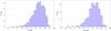 |
Fig. 1 Distribution of the G magnitudes of ICRF2 sources with calibrated photometric data in the auxiliary quasar table. Left: all 2152 sources. Right: the 260 defining sources. |
3.1. G magnitudes
An important first result derived from the data concerns the photometric properties of ICRF sources in the Gaia G band. For the first time, magnitudes are obtained for practically all the optical counterparts of the ICRF2 sources brighter than G ≃ 20.7. In the present list of 2191 sources there are 39 for which no G magnitudes were derived for Gaia DR1, although they all have good astrometric solutions5. The magnitude distribution of the remaining 2152 sources is shown in the left panel of Fig. 1 and in the right panel for the subset of 260 defining sources. The shape of the fall-off for G ≳ 20 is at least partly an instrumental effect due to the decreasing detection probability for fainter sources.
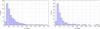 |
Fig. 2 Frequency distribution of the formal uncertainties in right ascension (σα ∗) of the optical positions of ICRF2 sources. The distributions are cut at 5 mas for clarity. Left: all 2191 sources (2090 with σα ∗< 5 mas). Right: the 262 defining sources (254 with σα ∗< 5 mas). |
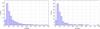 |
Fig. 3 Frequency distribution of the formal uncertainties in declination (σδ) of the optical positions of ICRF2 sources. The distributions are cut at 5 mas for clarity. Left: all 2191 sources (2100 with σδ< 5 mas). Right: the 262 defining sources (254 with σδ< 5 mas). |
3.2. Formal uncertainties of the positions
The distributions of the formal uncertainties σα ∗ and σδ in the auxiliary quasar solution are shown in Figs. 2, 3, respectively. The median value is 0.62 mas in right ascension and 0.56 mas in declination when all 2191 sources are considered, and 0.51 mas and 0.46 mas for the subset of 262 defining sources. These systematic differences in precision can be explained by Gaia’s scanning law and the fact that the defining sources are on average 0.3 mag brighter than the non-defining sources.
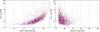 |
Fig. 4 Formal uncertainties of the optical positions of ICRF sources versus magnitude and number of observations per source. σpos, max refers to the semi-major axis of the error ellipse in position. Left: position uncertainty versus the G magnitude for 2152 sources with calibrated photometry. Right: position uncertainty of the 2191 sources versus the number of detections (field-of-view transits) used in the astrometric solution. Symbols show defining sources as blue squares, non-VCS sources as red crosses, and VCS-only sources as pale grey plus signs. |
Because of Gaia’s scanning law and the relatively small number of observations used in the present solutions, there is a high degree of correlation between α and δ for many of the sources. A better measure of the positional uncertainty could then be the semi-major axis of the error ellipse, σpos, max, which can be computed from σα ∗, σδ, and the correlation coefficient between α and δ (see Eq. (9) in Lindegren et al. 2016). Figure 4 shows scatter plots of σpos, max versus the G magnitude (left) and the number observations (right). The three groups of ICRF sources are shown with different symbols.
The expected increasing trend from the photon noise is very clear for the fainter sources in the left panel of Fig. 4. For G< 17 there is an accuracy floor around 0.25 mas due mainly to the limited performance of the instrument calibration in this release. There are, however, approximately 200 sources for which σpos, max is much higher than typical for their magnitudes. This could have several different causes, for example a small number of observations or a poor time sampling inadequate for the astrometric solution; this also could be due to source confusion in the initial matching of the detections or to a reduced detection probability for faint sources. Source structure, including an extended distribution of light from the host galaxy, is another possible explanation in some cases. Most of the outliers in the left panel of Fig. 4 can be explained by a small number of observations; as shown in the right panel, large positional uncertainties are much more common for sources with less than 10−15 matched detections.
4. Comparison of the optical and radio positions
In this section we compare the optical positions of the ICRF sources, as obtained in the Gaia auxiliary quasar solution, with their reference values in the radio domain taken from ICRF2 (Fey et al. 2015). Coordinate differences in right ascension and declination are computed as  (1)from which the angular separation between the two positions is obtained as
  (2)The small-angle approximation implicit in these formulae is perfectly adequate for our purpose, where position differences are <150 mas and consequently second-order effects <0.1 μas.
 |
Fig. 5 Distribution of the differences in right ascension between the Gaia solution and the ICRF2 positions. Left: the 2054 solutions closer than 10 mas to their radio position. Right: same for the 258 defining sources. |
 |
Fig. 6 Distribution of the differences in declination between the Gaia solution and the ICRF2 positions. Left: the 2054 solutions closer than 10 mas to their radio position. Right: same for the 258 defining sources. |
4.1. Position differences as angles
We consider first the position differences expressed as angles (in mas), that is without any scaling by their uncertainties or selection based on the uncertainties. The results are given in a series of diagrams showing the distributions of the coordinate differences and positional separations both for the whole set of 2191 sources and for the subset of defining sources. This separate consideration is mandatory given the different range of uncertainties in the ICRF2 positions for the defining or non-defining sources (Sect. 2.1).
The comparison is made under the assumption that the Gaia identification actually points to the matched ICRF source and therefore that when a difference is found between the two positions (radio and optical), it refers to the same source. It is clear, however, that for the largest separations, above a few tens of mas, a misidentification is possible and is not necessarily due to a flaw in the Gaia cross-matching, but more likely to the lack of a true optical counterpart within the detection range of Gaia. This will be investigated in later releases when more observations have been collected. Some sources have a relatively large uncertainty in ICRF2 (more than 5−10 mas), which could also be an explanation, in particular when the optical position is more accurate. The uncertainties are taken into account in the normalised comparisons (Sect. 4.2).
4.1.1. Coordinate differences
Histograms of the differences in right ascension and declination are shown, respectively, in Figs. 5 and 6. In each figure the left panel shows the distribution for all sources, the right panel shows the subset of defining sources. For better visibility only the central parts (within ± 10 mas) of the distributions are shown; the number of sources beyond this limit is given in the figure legends.
The median Δα ∗ for the whole sample is + 0.038 ± 0.022 mas. The standard width of the distribution estimated by the robust scatter estimate 6 (RSE) is 1.50 mas, while the non-robust sample standard deviation including the wings goes to 6.35 mas. The corresponding values for the defining subset are + 0.015 ± 0.038 mas for the median, 0.74 mas for the RSE, and 3.23 mas for the sample standard deviation. The agreement with the defining sources is obviously better owing to the better quality of this subset in the ICRF2. It is important to note that the Gaia frame has been aligned with the ICRF2 and that any bias in right ascension would therefore be absorbed by the orientation about the z-axis. However, the (robust) standard widths are good indicators of the quality of agreement between the two catalogues.
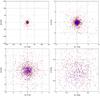 |
Fig. 7 Scatter plot of position differences in right ascension and declination (Gaia minus ICRF2). Top left: all 2191 sources. Top right: the 2069 sources within ± 10 mas in both coordinates. Bottom left: the 1742 sources within ± 3 mas in both coordinates. Bottom right: the 1069 sources within ± 1 mas in both coordinates. Symbols show defining sources as blue squares, non-VCS sources as red crosses, and VCS-only sources as grey plus signs. |
In declination the median Δδ for the whole sample is −0.069 ± 0.021 mas, the RSE 1.85 mas, and the sample standard deviation 7.99 mas. For the defining subset the median is −0.136 ± 0.032 mas, the RSE is 0.70 mas, and the sample standard deviation 3.21 mas. The bias of ≃−0.1 mas in declination is statistically significant and may be related to the (ecliptic) north-south asymmetry of systematics noted in Gaia DR1 parallax data (e.g. Appendix C in Lindegren et al. 2016). The reference frame alignment using a solid rotation (orientation) cannot remove a possible bias in declination7.
The plots in Fig. 7 show scatter plots of (Δα ∗ ,Δδ), colour-coded for the different categories of ICRF sources. The upper left plot goes up to ± 150 mas in each coordinate and therefore contains all 2191 sources. It shows primarily the few sources well outside the saturated centre where most of the sources are concentrated with overlapping markers. There are two obvious outliers among the defining sources (blue squares); they are discussed in Sect. 4.3. The upper right plot gives the distribution for the 2069 sources with coordinate differences within ± 10 mas. Here it is clearly seen that the defining sources, as expected, are more strongly concentrated around the centre than the non-VCS sources (red crosses), while the VCS-only sources (grey plus signs) have the largest spread. However, there are some 10−15 defining sources outside the central distribution that should be examined individually for possible contamination by the host galaxy or other anomalies. The lower left plot in Fig. 7 extending to ± 3 mas shows more detail near the centre, but the distribution remains remarkably symmetric even at the highest resolution. The lower right plot in Fig. 7 is a close-up view of the very central region within ± 1 mas in each coordinate and shows again the predominance of defining sources and the significant fraction of sources in the very inner zone at a few 0.1 mas from the centre. The very small bias in declination is now visible with more sources in the negative values of Δδ. The proportion of defining sources (blue squares) increases with resolution, but in all three plots the optical and radio positions are statistically in very good agreement for all three categories of sources despite the larger uncertainties in the radio data for the non-defining and especially the VCS-only sources.
4.1.2. Angular separations
Table 1 gives the overall statistics of the angular separation (ρ) between the optical and radio positions, subdivided according to the type of ICRF source. The table shows that 94% of the optical positions are within 10 mas of the radio position of the associated ICRF2 source. This is quite remarkable given the limited time coverage and the numerous limitations of the astrometric solutions for Gaia DR1 as explained in Lindegren et al. (2016). For the defining sources the percentage is even higher (98%). There is in fact a very consistent pattern in that the fraction of separations within a given limit (ρmax) is always higher for the defining sources than for the non-VCS sources, which in turn have a higher fraction than the VCS-only sources. Since the distinction between the three categories is irrelevant for Gaia (cf. Fig. 4), this confirms the difference in the quality of the radio positions expressed by the quoted uncertainties in ICRF2.
Number of ICRF sources with angular separations ρ<ρmax between the optical and radio positions.
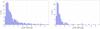 |
Fig. 8 Distribution of the angular distances between the Gaia solution and the ICRF2 positions. Left: the 2054 solutions closer than 10 mas to their radio position. Right: same for the 258 defining sources. |
Figure 8 shows the distribution of separations in graphical form. The difference between the whole set and the set of defining sources is even more conspicuous than for the coordinate differences. The median is 1.16 mas in one case and only 0.61 mas in the other. As mentioned earlier this is primarily due to the very different quality in the ICRF2 between the defining sources and the rest of the catalogue and confirms a well-known feature of the ICRF2 with fully independent observations.
4.2. Normalised differences
In this section we discuss the positional differences scaled by their standard uncertainties. We define the normalised coordinate differences as  (3)where the ICRF values are taken from the ICRF2 catalogue. The scaled analogue of ρ will be defined later (Sect. 4.2.2).
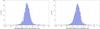 |
Fig. 9 Distribution of the normalised differences in right ascension (left) and declination (right) between the Gaia DR1 positions of 2191 ICRF sources and their radio positions. The histograms are cut at ± 8 in the normalised differences, leaving out 28 sources with | Xα | > 8 and 28 sources with | Xδ | > 8. The black curves are the expected centred normal distribution of unit standard deviation. |
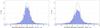 |
Fig. 10 Distribution of the differences in right ascension (left) and declination (right) between the Gaia DR1 positions of 2191 ICRF sources, normalised by the uncertainties of the Gaia data. The histograms leave out 97 sources with | Δα ∗ /σα ∗ | > 8 and 154 sources with | Δδ/σδ | > 8. The black curves are the expected centred normal distribution of unit standard deviation. |
4.2.1. Normalised coordinate differences
Figure 9 shows the cores of the distributions of Xα and Xδ, leaving out only a few dozen points beyond the histogram boundaries. The histograms roughly follow the expected normal distribution of unit width, although there are clearly several tens of outliers in both histograms, and the negative bias in declination is clearly visible in the right histogram. The overall agreement is confirmed by the RSE, which is 1.01 in right ascension and 1.02 in declination. The outliers increase the sample standard deviations to 2.4 and 2.6, respectively.
The normalisation factors in Eq. (3) include the contributions from the uncertainties in both data sets (Gaia and ICRF). For comparison we show in Fig. 10 the corresponding plots when only the uncertainties in the Gaia data are included (obtained by setting σα ∗ , ICRF = σδ, ICRF = 0 in Eq. (3)). As expected, the resulting distributions are significantly wider (the RSE is 1.70 in α and 2.50 in δ), but the main difference is the much larger number of sources in the wings than when the combined uncertainties are used to scale the differences. These are primarily due to the non-defining sources for which the radio positions are often much more uncertain than the optical positions. The good overall agreement when the combined uncertainties are used suggests that the uncertainties quoted in ICRF2 for the non-defining sources are fairly reliable. Actually the true positional uncertainty of the VCS-only sources is probably difficult to ascertain with VLBI observations performed in a single session. The ongoing work to prepare ICRF3 with repeated observations of VLBA calibrators will be very useful in this respect (Gordon et al. 2016).
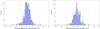 |
Fig. 11 Distribution of the normalised differences in right ascension (left) and declination (right) between the Gaia DR1 positions of 262 defining ICRF sources and their radio positions. The histograms are cut at ± 8 in the normalised differences, leaving out two sources with | Xα | > 8 and three sources with | Xδ | > 8. The black curves are the expected centred normal distribution of unit standard deviation. |
Focusing now on the defining sources, we show in Fig. 11 the distributions Xα and Xδ for the subset of 262 defining sources in the auxiliary quasar solution. For these sources the uncertainty coming from the ICRF2 is negligible, with a median around 0.06 mas, in comparison to the Gaia uncertainty, which has a median around 0.5 mas. The combined uncertainties in Eq. (3) are therefore dominated by the uncertainties from Gaia, and the distribution of the normalised differences is primarily a test of the realism of the Gaia uncertainties and of possible physical optical-radio offsets. The RSE of the normalised differences is 1.03 in right ascension and 1.05 in declination. The deviations of these values from 1.00 are not statistically significant: the uncertainties in RSE estimated by bootstrap are about 0.08. Considering the much smaller sample, the overall agreement with a normal distribution is about as good for the defining sources in Fig. 11 as for the whole sample in Fig. 9. The proportion of outliers is also similar, with about 5% defining sources beyond three standard deviations in either coordinate; the corresponding number for the whole sample is about 7%. The bias in declination is more apparent for the defining subset because of the smaller combined uncertainties.
If we disregard the bias in declination and a certain percentage of outliers, the distributions of the normalised differences for both defining and non-defining sources are in reasonable agreement with a normal distribution with zero mean and unit variance. The normalising factor only takes into account the statistical errors and does not include the possible additional noise coming from an actual optical-radio offset. If such an offset is present in most of the sources, it will be random in direction and will contribute to the observed dispersion of coordinate differences, thus increasing the RSE values. This increase would be more noticeable for the sources with small combined uncertainties. From the plots, despite the small number of sources usable for this purpose, it is already possible to state that if such offsets exist in the majority of the defining sources, they must be much less than 1 mas. The RSE values of 1.03−1.05 for the normalised differences of the defining sources, although insignificantly larger than one, set an upper limit of about 0.4 mas for the optical-radio offsets because otherwise the RSE values would be significantly larger than one. This is a statistical result, and does not preclude that the offsets are usually small and large only for a small fraction of the sources. By a similar reasoning it is possible to conclude that the stated uncertainties of the Gaia positions in general cannot be underestimated, in the quadratic sense, by more than about 0.4 mas.
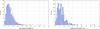 |
Fig. 12 Distribution of the normalised separations X (Eq. (4)) between the Gaia DR1 positions of ICRF sources and their radio positions. Left: all 2191 sources (36 have X> 10). Right: the 262 defining sources (three have X> 10). The black curve is the expected Rayleigh distribution. |
4.2.2. Normalised separations
When considering the normalised differences in both coordinates jointly, an obvious analogue of ρ in Eq. (2) is  . However, this quantity can be misleading when there are strong correlations between the errors in α and δ, which is often the case especially for the Gaia data. Indeed, for Gaussian errors the theoretical distribution of this quantity depends on the degree of correlation between the two coordinates. To take into account the correlation coefficients CGaia and CICRF in both data sets, we use the statistic
 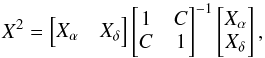 (4)where
 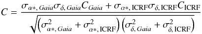 (5)is the correlation coefficient of the combined errors. For Gaussian errors we expect X2 to follow the chi-squared distribution with two degrees of freedom (see Appendix B for the mathematical details). Equivalently, the normalised separation X has a Rayleigh distribution, that is Pr(X>x) = exp(−x2/ 2). Figure 12 shows the distributions of X for all the ICRF sources and for the defining sources. The median value of X is 1.11 ± 0.02 for the whole sample of 2191 sources, and 1.28 ± 0.05 for the defining subset. Compared with the theoretical value (ln4)1/2 ≃ 1.18, the dispersion is slightly too large for the defining sources and too small for the whole sample. The decreasing trend is consistent when going from defining to non-VCS and VCS-only sources, with median values 1.28, 1.26, and 1.03, respectively. Since this trend is opposite to the variation of the formal uncertainties in ICRF2, it could be explained by a constant contribution from actual optical-radio offsets, or by the formal uncertainties in ICRF2 being overestimated for the VCS-only sources and possibly underestimated for the other sources. That the root cause of this trend is in the Gaia data seems less likely, as the three categories of ICRF sources have similar properties in the Gaia observations. The larger-than-expected median values for the defining and non-VCS sources could still be explained by an underestimation of the Gaia uncertainties, in which case the ICRF2 uncertainties of the VCS-only sources would have to be even more overestimated.
Concerning the tail of large normalised separations we note that, for the theoretical distribution, the expected number of points with X> 4.1 in a sample of size 2191 is less than 0.5. In reality we find 107 sources above this limit, including 11 defining sources. These can reasonably be considered as outliers requiring a more detailed analysis.
4.3. Deviating cases
We now consider the sources whose optical positions in the Gaia data deviate markedly from the radio positions of the matched ICRF sources, either in angular separation (ρ) or in normalised separation (X). Figure 13 is a plot of ρ versus X for all 2191 sources. In Sect. 4.2.2 we concluded that sources with X> 4.1 have a larger separation than expected from the combined formal uncertainties, and can therefore be considered as deviating cases on purely statistical grounds. This subset contains 107 sources, which is 5% of the whole sample.
The sources with atypically large angular separations are also interesting, however, for reasons more related to the physical properties of the sources, their environment on the sky, and the resolution of the Gaia instrument. Here it is much harder to motivate a priori any specific limit in angular separation beyond which a source merits special attention. Somewhat arbitrarily, we chose to look at the sources with ρ> 10 mas, a value significantly larger than the typical combined uncertainty. There are 137 sources that are singled out by this criterion, a number small enough to think of a case-by-case investigation.
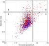 |
Fig. 13 Angular separation ρ versus normalised separation X for 2191 ICRF sources. Defining sources are shown as blue squares, non-VCS sources as red crosses, and VCS-only sources as pale grey plus signs. The four regions labelled A, B, C, and D are separated by ρ = 10 mas and X = 4.1. |
The limits in X and ρ divide the 2191 ICRF sources into four categories, corresponding to the regions labelled A, B, C, and D in Fig. 13, and which are treated separately below. It was not possible to investigate every deviating source; only a few representative or extreme cases are discussed in some detail. Individual cases were examined using online resources available through the Strasbourg astronomical Data Center (CDS), including the Sloan Digital Sky Survey (SDSS; York et al. 2000; Eisenstein et al. 2011) and the Two Micron All Sky Survey (2MASS; Skrutskie et al. 2006).
-
A.
This is the unproblematic category where both ρ and X are unremarkable. It contains 1982 sources (247 defining, 562 non-VCS, and 1173 VCS-only sources), which will not be discussed further.
-
B.
In this category the angular separation exceeds 10 mas, but X is still below the limit which means that the large separation may not be statistically significant. This category contains 102 sources (4 defining, 24 non-VCS, and 74 VCS-only sources). The four defining sources were examined individually and are listed in order of decreasing angular separation:
-
ICRF J121546.7-173145 (ρ = 58.9 mas) is within 40′′ of the 2nd magnitude star γ Corvi. This produces a large glare around the image, increasing the background noise and generating many false detections. It is possible that Gaia will never deliver a good solution for this source.
-
ICRF J173302.7-130449 (ρ = 27.3 mas) is at 30′′ from a star of magnitude 7.5. It is not obvious how much trouble this produced in the Gaia detection, but the observation record shows that the detections were not always matched to the same Gaia source, which supports the conjecture that false detections have contaminated the solution.
-
ICRF J144553.3-162901 (ρ = 12.8 mas) is a rather poorly observed source with only eight matched detections and a positional uncertainty around 15 mas in the Gaia data. The optical source is isolated in the SDSS and 2MASS surveys.
-
ICRF J023945.4-023440 (ρ = 10.1 mas) is also a poorly observed source with seven matched detections and Gaia uncertainties around 8 mas. Again, the optical source is isolated in the SDSS and 2MASS surveys.
The most deviating non-VCS source in this category is ICRF J054138.0−054149 (ρ = 117.9 mas, X = 1.3). The auxiliary quasar solution has large uncertainties for this source, although there is a good number of matched detections. No nearby bright star or host galaxy is visible in the 2MASS or SDSS survey, but the source is very faint for Gaia at G = 20.7.
The Gaia uncertainties for these five sources are characterised by very elongated error ellipses (axis ratios in the range 9 to 185) caused by poor coverage in terms of the scanning directions. This will definitely improve when more observations are used in the solution and at least the last two defining sources should then get good positions from Gaia.
-
-
C.
This category contains sources with angular separations exceeding 10 mas that are statistically significant in relation to the formal uncertainties. This is where we are most likely to find a clear reason for the offset of the optical centre from the radio centre, caused for example by the host galaxy or a nearby faint star. The category includes 35 sources (17 non-VCS and 18 VCS-only sources), with one defining source just below the separation limit (see category D). The four non-VCS sources with the highest significance are listed in order of decreasing X:
-
ICRF J013741.2+330935 (X = 70, ρ = 54 mas) is 3C 48 embedded in the extended galaxy SDSS9 J013741.30+330935.0;
-
ICRF J133037.6+250910 (X = 55, ρ = 128 mas) is 3C 287. On SDSS there are two optical objects of comparable magnitude (around 18) at 3′′ from each other, with the ICRF position roughly coinciding with the brighter object. From the SDSS images it is difficult to determine if this object is extended. The optical position from Gaia is offset from the radio position by 128 mas towards the north-east and away from the other object, but it is difficult to see how such a faint object at 3′′ could perturb the Gaia measurements;
-
ICRF J120321.9+041419 (X = 53, ρ = 45 mas) is at the centre of a weak extended galaxy image, SDSS9 J120321.93+041419.0, larger than 1′′ on SDSS images;
-
ICRF J114722.1+350107 (X = 32, ρ = 19 mas) is at the centre of an extended galaxy image which is 10′′ in diameter but with a luminous core. The image has a high background for Gaia with a bright point-like core, so Gaia performs nominally well, but the optical centre could be displaced by the surrounding bright distribution of light.
The Gaia solutions for these sources are formally good, with uncertainties below 1 mas and moderate axis ratios (in the range 1.4 to 4).
-
-
D.
This category contains sources with moderate offsets (1−10 mas) that are nevertheless significant thanks to the small formal uncertainties in both the optical and radio data. It contains 72 sources (11 defining, 37 non-VCS, and 24 VCS-only sources). The most discrepant defining source is ICRF J155850.2-643229 (X = 32, ρ = 9.97 mas). The relatively bright source seen by Gaia (G = 16.3) could be the central part of the galaxy 2MASX J15585027-6432298 with a total magnitude around 14 in the Gaia band. The 10 mas offset corresponds to a shift of the optical centre by only 15 pc at the distance of the galaxy, which is not unreasonable if the optical emission associated with the radio source is not strong.
Several of the sources in categories C and D clearly merit further investigation using high-resolution imaging.
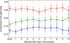 |
Fig. 14 Components of the glide and their errors (x, y, and z components are shown in red, green, and blue, respectively) for different largest VSH orders used in the fit (“alone” means that the three glide parameters are fitted without the three rotation parameters). The values correspond to the weighted solutions with all sources in region A as in Table 2. |
Global differences between the Gaia DR1 positions of ICRF sources and their positions in ICRF2, expressed by the orientation and glide parameters.
4.4. Large-scale systematic differences
In this section we compare the two sets of positions in search of general large-scale patterns, like a global rotation or a glide, which could explain a fraction of the position differences. The positional reference frame of Gaia DR1, based on the auxiliary quasar solution, has been aligned with ICRF2 as explained in the Gaia DR1 astrometry paper (Lindegren et al. 2016). We therefore do not expect to see any systematic difference that could be represented by a solid rotation. However, the presence of a small difference in declination, noted in Sect. 4.1.1, does suggest other kinds of systematics that should be examined.
Our analysis is based on the expansion of the vector field of the differences (two components in the tangent plane of the celestial sphere at the location of each source) on a set of vector spherical harmonics (VSH) as explained in Mignard & Klioner (2012) or Vityazev & Tsvetkov (2014). Instead of fitting the differences on a model including the rotation, the positional differences are expanded on a set of orthogonal functions up to a certain degree lmax. The global rotation and the glide (the vector field locally perpendicular to the rotation field; see Sects. 4.2, 4.3 in Mignard & Klioner 2012) are extracted from the harmonics of degree l = 1. This procedure is more general than the alignment since it includes higher order terms that could otherwise project on the rotation when this simplified model is used in isolation. This test is therefore an independent check of the initial alignment as well as a search for potential large-scale systematics.
The results shown in Table 2 are very satisfactory for the present state of the Gaia data. In particular they confirm the absence of global rotation at least on the level of 0.05 mas. However, they do indicate a glide of about 0.13 mas, consistent with the declination difference mentioned above. The values of the glide parameters are rather stable with respect to the parameters of the fit as illustrated by Fig. 14. While it is not possible to tell from this comparison alone whether the glide results from a distortion of the Gaia DR1 reference frame or of the ICRF, we note that the validation of the Gaia DR1 astrometry has revealed many sorts of systematics at the level of 0.1−0.3 mas (Arenou et al. 2016; Lindegren et al. 2016). It is therefore quite possible that the reference frame of Gaia DR1 is distorted by a similar amount. Apart from the glide, the VSH expansion shows few terms of higher order (e.g. l = 3) with significant, albeit very small, amplitudes.
Part of the observed glide component may be caused by the apparent proper motion of quasars induced by the galactocentric acceleration of the solar system barycentre (Fanselow 1983; Bastian 1995; Sovers et al. 1998; Kovalevsky 2003; Titov & Lambert 2013). This effect should produce a gradually increasing distortion of the ICRF2 positions in the form of a glide vector directed towards the Galactic Centre and with an amplitude proportional to the time elapsed since the mean epoch of the VLBI observations. Using galactic parameters from Reid et al. (2009), and taking the mean epoch of ICRF2 to be 13.7 years earlier than Gaia DR1, the expected amplitude of the distortion is 0.074 mas. The observed glide is almost twice as large and directed ~ 30° away from the Galactic Centre. It is therefore probably a combination of the galactic effect with some other systematics. The unexplained (non-galactic) component is mainly directed along the z-axis.
Conceptually, the two reference frames (Gaia in the visible and ICRF2 in the radio domain) are materialisations of the same reference system. Our test shows that this holds globally at a level of 0.2 mas, again a very satisfactory situation for this first Gaia solution.
5. Discussion of the optical-radio offsets
The non-coincidence of the optical and radio centres of ICRF sources has long been a concern for the achievement of an accurate optical reference frame (e.g. da Silva Neto et al. 2002; and Makarov et al. 2012). Although there are good theoretical reasons to expect that the offsets are generally small (<1 mas; e.g. Kovalev et al. 2008; and Popović et al. 2012), observational studies tend to find much larger effects (e.g. Taris et al. 2011; Orosz & Frey 2013, and the surveys discussed below).
Based on deep CCD imaging of the optical counterparts of ICRF sources, linked to the Hipparcos/Tycho-2 reference frame, Zacharias & Zacharias (2014) hypothesised the existence of a detrimental, astrophysical, random noise (DARN) optical-radio offset on a level of ≃10 mas. Comparing Gaia DR1 optical-radio coordinate differences with those in Tables 4 and 5 in the USNO survey we find little or no correlation for the ~320 sources in common. While the RSE of the coordinate differences for the common sources is less than 1 mas in Gaia DR1, it is 20−30 mas in the USNO survey. A similar comparison with the Rio survey (Assafin et al. 2013) gives the same result. On the other hand, there is a clear (if rather weak) positive correlation between the differences in the USNO and Rio surveys, although different instruments were used.
Clearly most of the offsets found in the Rio and USNO surveys must have other causes than a real non-coincidence of the optical and radio centres. A reasonable hypothesis is that the offsets are to a large extent caused by the spatially correlated (i.e. systematic, mainly zonal) errors in the Tycho-2 proper motions revealed by Gaia (see Appendix C.1 in Lindegren et al. 2016). The errors, on a level of 2−6 mas yr-1, are much larger than assumed by Zacharias & Zacharias (2014), and could contribute offsets up to ~50 mas over the ~10 year epoch difference between the surveys and Hipparcos/Tycho-2. Although a DARN effect will surely exist at some level, it must in general be well below 1 mas.
6. Conclusions
As part of Gaia DR1 we present the optical positions of 2191 Gaia sources matched to ICRF2 sources, including 262 of the defining sources in ICRF2. These positions, which come from the special auxiliary quasar solution, are shown to be more accurate than the positions from the secondary solution given elsewhere in Gaia DR1. Magnitudes in Gaia’s G band are given for 2152 of the sources (260 defining). The properties of the optical data are discussed and detailed comparisons made between the optical and radio positions of the ICRF sources. The main conclusions are the following:
-
The G magnitudes span a range from 12.4 to 21.0 mag with the bulk of sources between 17 and 20 mag.
-
The formal accuracy of the optical positions has a floor at ~0.25 mas for G< 17 mag, gradually increasing to a few mas at G = 20. There is no systematic difference between defining and non-defining ICRF sources in terms of their optical accuracies versus magnitude.
-
The overall agreement between the optical and radio positions is excellent: the angular separation is <1 mas for 44% of the sources and <10 mas for 94% of the sources. For the defining sources the corresponding numbers are 71% and 98%.
-
Analysis of the large-scale systematic differences between the optical and radio positions in terms of VSH reveals no significant components except for a glide of amplitude ~0.15 mas.
-
The angular separations are in general consistent with the combined formal uncertainties in ICRF2 and the Gaia data, supporting the claimed accuracies. The uncertainties of the radio positions of VCS-only sources in ICRF2 may be overestimated.
-
For most of the 6% sources with angular separations above 10 mas the optical-radio offsets are consistent with the stated formal uncertainties of the data, but for a quarter of them the offsets are statistically significant. Individual examination of a number of these cases shows that a likely explanation for the offset can often be found, for example in the form of a bright host galaxy or nearby star.
-
Among the sources with good optical and radio astrometry we found no indication of physical optical-radio offsets exceeding a few tens of mas. For most sources the true offsets are likely to be less than 1 mas.
The last result is very encouraging for the future alignment of the very accurate optical reference frame to be built from Gaia observations and the corresponding radio frame, using common sources in two very different wavelength domains.
The exception is the Hipparcos quasar HIP 60936 = 3C 273 = ICRF J122906.6+020308, where the position comes from the primary (Tycho−Gaia) astrometric solution of Gaia DR1. For simplicity we ignore this exception in the following, and refer to the data as coming from the auxiliary quasar solution.
This measures the amount of noise, including calibration errors, that must be assumed to exist in the elementary observations in addition to the photon noise in order to account for the dispersion of residuals in the astrometric solution (Lindegren et al. 2012).
The auxiliary quasar table is available in machine-readable form from http://archives.esac.esa.int/gaia/
Inter-source correlations are expected to be negligible, given the large angular separation of ICRF sources (several degrees) and the scanning geometry of Gaia. Empirically, we found that the positional differences between Gaia DR1 and ICRF2 have insignificant correlations, except on scales ≲ 10° where they may reach 0.04.
Straight inspection of the (uncalibrated) fluxes in the pre-processing for these 39 sources indicates that their magnitudes range from 17.5 to 20.5.
The RSE is defined as  times the distance between the 10th and 90th percentiles. For a normal distribution it equals the standard deviation.
After the submission of the paper the authors learnt independently from P. Charlot and Ch. Jacobs (priv. comm.) that a similar bias is seen between the ICRF2 and the preliminary solution of ICRF3.
Acknowledgments
This work has made use of data from the ESA space mission Gaia, processed by the Gaia Data Processing and Analysis Consortium (DPAC). This research has made use of Aladin sky atlas and the Simbad database developed at CDS, Strasbourg Observatory, France. We are grateful to the developers of TOPCAT (Taylor 2005) for their software. Funding for the DPAC has been provided by national institutions, in particular the institutions participating in the Gaia Multilateral Agreement. The Gaia mission website is http://www.cosmos.esa.int/gaia. The authors are members of the Gaia DPAC. This work has been supported by the European Space Agency in the framework of the Gaia project; the Centre National d’Études Spatiales (CNES); the German Aerospace Agency DLR under grants 50QG0501, 50QG1401 50QG0601, 50QG0901, and 50QG1402; and the Swedish National Space Board. The authors are very grateful to Chris Jacobs for his constructive review and thoughtful remarks, which helped to improve the paper.
References
- Andrei, H., Antón, S., Taris, F., et al. 2014, in Journées 2013 Systèmes de référence spatio-temporels, ed. N. Capitaine, 84 [Google Scholar]
- Arenou, F., Luri, X., Babusiaux, C., et al. 2016, A&A, submitted (Gaia SI) [Google Scholar]
- Assafin, M., Vieira-Martins, R., Andrei, A. H., Camargo, J. I. B., & da Silva Neto, D. N. 2013, MNRAS, 430, 2797 [NASA ADS] [CrossRef] [Google Scholar]
- Bailer-Jones, C. A. L., Andrae, R., Arcay, B., et al. 2013, A&A, 559, A74 [NASA ADS] [CrossRef] [EDP Sciences] [Google Scholar]
- Bastian, U. 1995, in Future Possibilities for astrometry in Space, eds. M. A. C. Perryman, & F. van Leeuwen, ESA SP, 379, 99 [Google Scholar]
- Beasley, A. J., Gordon, D., Peck, A. B., et al. 2002, ApJS, 141, 13 [NASA ADS] [CrossRef] [Google Scholar]
- da Silva Neto, D. N., Andrei, A. H., Vieira Martins, R., & Assafin, M. 2002, AJ, 124, 612 [NASA ADS] [CrossRef] [Google Scholar]
- Eisenstein, D. J., Weinberg, D. H., Agol, E., et al. 2011, AJ, 142, 72 [Google Scholar]
- Fabricius, C., Bastian, U., Portell, J., et al. 2016, A&A, 595, A3 (Gaia SI) [Google Scholar]
- Fanselow, J. L. 1983, Observation Model and parameter partial for the JPL VLBI parameter Estimation Software MASTERFIT-V1.0, Tech. Rep. [Google Scholar]
- Fey, A. L., Gordon, D., Jacobs, C. S., et al. 2015, AJ, 150, 58 [NASA ADS] [CrossRef] [Google Scholar]
- Gaia Collaboration (Prusti, T., et al.) 2016, A&A, 595, A1 (Gaia SI) [NASA ADS] [CrossRef] [EDP Sciences] [Google Scholar]
- Gordon, D., Jacobs, C., Beasley, A., et al. 2016, AJ, 151, 154 [NASA ADS] [CrossRef] [Google Scholar]
- Kovalev, Y. Y., Petrov, L., Fomalont, E. B., & Gordon, D. 2007, AJ, 133, 1236 [NASA ADS] [CrossRef] [Google Scholar]
- Kovalev, Y. Y., Lobanov, A. P., Pushkarev, A. B., & Zensus, J. A. 2008, A&A, 483, 759 [NASA ADS] [CrossRef] [EDP Sciences] [Google Scholar]
- Kovalevsky, J. 2003, A&A, 404, 743 [NASA ADS] [CrossRef] [EDP Sciences] [Google Scholar]
- Lindegren, L., Lammers, U., Hobbs, D., et al. 2012, A&A, 538, A78 [NASA ADS] [CrossRef] [EDP Sciences] [Google Scholar]
- Lindegren, L., Lammers, U., Bastian, U., et al. 2016, A&A, 595, A4 (Gaia SI) [NASA ADS] [CrossRef] [EDP Sciences] [Google Scholar]
- Ma, C., Arias, E. F., Eubanks, T. M., et al. 1998, AJ, 116, 516 [NASA ADS] [CrossRef] [Google Scholar]
- Ma, C., Arias, E. F., Bianco, G., et al. 2009, IERS Technical Note, 35 [Google Scholar]
- Makarov, V., Berghea, C., Boboltz, D., et al. 2012, Mem. Soc. Astron. Italiana, 83, 952 [NASA ADS] [Google Scholar]
- Michalik, D., & Lindegren, L. 2016, A&A, 586, A26 [NASA ADS] [CrossRef] [EDP Sciences] [Google Scholar]
- Mignard, F., & Klioner, S. 2012, A&A, 547, A59 [NASA ADS] [CrossRef] [EDP Sciences] [Google Scholar]
- Orosz, G., & Frey, S. 2013, A&A, 553, A13 [NASA ADS] [CrossRef] [EDP Sciences] [Google Scholar]
- Petrov, L., Kovalev, Y. Y., Fomalont, E. B., & Gordon, D. 2008, AJ, 136, 580 [NASA ADS] [CrossRef] [Google Scholar]
- Popović, L. Č., Jovanović, P., Stalevski, M., et al. 2012, A&A, 538, A107 [NASA ADS] [CrossRef] [EDP Sciences] [Google Scholar]
- Reid, M. J., Menten, K. M., Zheng, X. W., et al. 2009, ApJ, 700, 137 [NASA ADS] [CrossRef] [Google Scholar]
- Skrutskie, M. F., Cutri, R. M., Stiening, R., et al. 2006, AJ, 131, 1163 [NASA ADS] [CrossRef] [Google Scholar]
- Smart, R. L., & Nicastro, L. 2013, VizieR Online Data Catalog, I/324 [Google Scholar]
- Sovers, O. J., Fanselow, J. L., & Jacobs, C. S. 1998, Rev. Mod. Phys., 70, 1393 [NASA ADS] [CrossRef] [Google Scholar]
- Taris, F., Souchay, J., Andrei, A. H., et al. 2011, A&A, 526, A25 [NASA ADS] [CrossRef] [EDP Sciences] [Google Scholar]
- Taylor, M. B. 2005, in Astronomical Data Analysis Software and Systems XIV, eds. P. Shopbell, M. Britton, & R. Ebert, ASP Conf. Ser., 347, 29 [Google Scholar]
- Titov, O., & Lambert, S. 2013, A&A, 559, A95 [NASA ADS] [CrossRef] [EDP Sciences] [Google Scholar]
- Vityazev, V. V., & Tsvetkov, A. S. 2014, MNRAS, 442, 1249 [NASA ADS] [CrossRef] [Google Scholar]
- York, D. G., Adelman, J., Anderson, Jr., J. E., et al. 2000, AJ, 120, 1579 [Google Scholar]
- Zacharias, N., & Zacharias, M. I. 2014, AJ, 147, 95 [NASA ADS] [CrossRef] [Google Scholar]
Appendix A: Identification of ICRF sources in the secondary solution of Gaia DR1
Apart from the auxiliary quasar table, all positional data in Gaia DR1 for faint sources come from the secondary solution. For most of the sources in the auxiliary quasar table slightly different positions from the secondary solution can be found. In this appendix we briefly consider the optical positions of ICRF sources in the secondary solution, even though they are not used in the rest of the paper.
Searching the secondary solution of Gaia DR1 for positional matches to the 3414 radio positions in ICRF2 results in 2299 matches within 150 mas (the same limit as was used in Sect. 2.4). All of the matches are unique in the sense that there is at most one optical source within 150 mas of the radio source. Among the ICRF sources there are 260 defining, 657 non-VCS, and 1382 VCS-only sources.
Comparing the optical positions from the two tables (auxiliary and secondary) with the matched ICRF2 positions clearly demonstrates the superiority of the auxiliary quasar solution. For example, the median separation (Eq. (2)) is ρ = 1.2 mas for the auxiliary quasar table and 1.8 mas for the secondary table. The difference is even more pronounced for the defining sources, where the median separations are 0.6 mas (auxiliary) and 1.1 mas (secondary). These results do not change significantly if we only consider the subset of 2135 ICRF2 sources (of which 256 are defining) that appear in both tables.
Not only are the positions from the auxiliary quasar solution more accurate than in the secondary solution, but the associated standard uncertainties also appear to be more reliable in the auxiliary solution. This can be seen from the robust dispersion (RSE) of the normalised coordinate differences Xα, Xδ (Eq. (3)). For the auxiliary quasar solution the dispersion is close to one, as expected, even for the defining sources (see Figs. 9 and 11). For the secondary solution the dispersion is about 10% higher for the whole sample and 30% higher for the defining sources. This is a strong indication that the positional uncertainties are severely underestimated in the secondary solution, which is not the case for the auxiliary table. There are thus good reasons to restrict the detailed analysis of the optical-radio differences to the auxiliary quasar table.
As already mentioned, the two tables have 2135 ICRF2 sources in common, which means that the secondary table contains 2299−2135 = 164 ICRF2 sources that are not listed in the auxiliary table. Conversely, the auxiliary table contains 2191−2135 = 56 ICRF2 sources not listed in the secondary table. The relation between the two tables is even more complicated: among the 2135 ICRF2 sources that appear in both tables, 56 have different Gaia source identifiers in the two tables. This means that the auxiliary and secondary positions for these 56 ICRF2 sources were computed from disjoint subsets of the Gaia detections (cf. Sect. 2.2). Complications of this sort happened in Gaia DR1 because of the imperfect state of the initial source list and the relatively large attitude and calibration errors in the initial processing steps, but in later releases they will eventually be eliminated.
Appendix B: Derivation of Eq. (4)
Appendix B.1: Covariance for the differences of two random vectors
Consider two independent k-dimensional random vectors x1 and x2 with mutlivariate normal distribution with means μ1,μ2 and covariance matrices respectively Σ1 and Σ2. Each distribution is then  . Without changing the subsequent argument, μ1 = μ2 = 0 can always be assumed. As a consequence of the independence of the two random vectors, the joint distribution of the vector of 2k-dimension x = [x1,x2] T also has a multivariate normal distribution with zero mean and covariance matrix,
  (B.1)where Σ∗ is a 2k × 2k positive definite symmetric matrix. We now introduce the k-dimensional random vector
  (B.2)This transformation can also be written as linear mapping from ℛ2k to ℛk as
  (B.3)where B is a k × 2k matrix, built with the k-dimensional unit matrix Ik,
  (B.4)Therefore, the probability distribution of y is
  , where the covariance matrix is given by
  (B.5)or more trivially
  (B.6)a generalisation of the addition of the variances for two scalar independent variables.
For a normal distribution of a k-dimensional random vector x the quadratic form  (B.7)follows a χ2 distribution with k degrees of freedom.
Appendix B.2: Application to k = 2
This is the case of interest in this paper with the differences between Gaia and ICRF2 respectively in right ascension and declination. Let x1 = (x1,y1) and x2 = (x2,y2), which yields successively  (B.8)and
 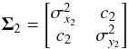 (B.9)and finally,
 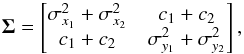 (B.10)where c1 = cov(x1,y1) and c2 = cov(x2,y2), respectively the covariance between the errors in the ICRF2 and in the Gaia solution in right ascension and declination, and then xα = x2−x1 and xδ = y2−y1 for the two components of the positional differences.
The quadratic form 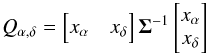 (B.11)therefore follows a χ2 distribution with 2 degrees of freedom or, equivalently,
  follows a standard Rayleigh distribution. An analytical inversion of Σ gives the same asEq. (4), although it is written with reduced variables with unit variances and the covariance identical to the correlation coefficient. Thus C in Eq. (5) is the same as
 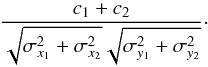 (B.12)
All Tables
Number of ICRF sources with angular separations ρ<ρmax between the optical and radio positions.
Global differences between the Gaia DR1 positions of ICRF sources and their positions in ICRF2, expressed by the orientation and glide parameters.
All Figures
|
Fig. 1 Distribution of the G magnitudes of ICRF2 sources with calibrated photometric data in the auxiliary quasar table. Left: all 2152 sources. Right: the 260 defining sources. |
| In the text | |
|
Fig. 2 Frequency distribution of the formal uncertainties in right ascension (σα ∗) of the optical positions of ICRF2 sources. The distributions are cut at 5 mas for clarity. Left: all 2191 sources (2090 with σα ∗< 5 mas). Right: the 262 defining sources (254 with σα ∗< 5 mas). |
| In the text | |
|
Fig. 3 Frequency distribution of the formal uncertainties in declination (σδ) of the optical positions of ICRF2 sources. The distributions are cut at 5 mas for clarity. Left: all 2191 sources (2100 with σδ< 5 mas). Right: the 262 defining sources (254 with σδ< 5 mas). |
| In the text | |
|
Fig. 4 Formal uncertainties of the optical positions of ICRF sources versus magnitude and number of observations per source. σpos, max refers to the semi-major axis of the error ellipse in position. Left: position uncertainty versus the G magnitude for 2152 sources with calibrated photometry. Right: position uncertainty of the 2191 sources versus the number of detections (field-of-view transits) used in the astrometric solution. Symbols show defining sources as blue squares, non-VCS sources as red crosses, and VCS-only sources as pale grey plus signs. |
| In the text | |
|
Fig. 5 Distribution of the differences in right ascension between the Gaia solution and the ICRF2 positions. Left: the 2054 solutions closer than 10 mas to their radio position. Right: same for the 258 defining sources. |
| In the text | |
|
Fig. 6 Distribution of the differences in declination between the Gaia solution and the ICRF2 positions. Left: the 2054 solutions closer than 10 mas to their radio position. Right: same for the 258 defining sources. |
| In the text | |
|
Fig. 7 Scatter plot of position differences in right ascension and declination (Gaia minus ICRF2). Top left: all 2191 sources. Top right: the 2069 sources within ± 10 mas in both coordinates. Bottom left: the 1742 sources within ± 3 mas in both coordinates. Bottom right: the 1069 sources within ± 1 mas in both coordinates. Symbols show defining sources as blue squares, non-VCS sources as red crosses, and VCS-only sources as grey plus signs. |
| In the text | |
|
Fig. 8 Distribution of the angular distances between the Gaia solution and the ICRF2 positions. Left: the 2054 solutions closer than 10 mas to their radio position. Right: same for the 258 defining sources. |
| In the text | |
|
Fig. 9 Distribution of the normalised differences in right ascension (left) and declination (right) between the Gaia DR1 positions of 2191 ICRF sources and their radio positions. The histograms are cut at ± 8 in the normalised differences, leaving out 28 sources with | Xα | > 8 and 28 sources with | Xδ | > 8. The black curves are the expected centred normal distribution of unit standard deviation. |
| In the text | |
|
Fig. 10 Distribution of the differences in right ascension (left) and declination (right) between the Gaia DR1 positions of 2191 ICRF sources, normalised by the uncertainties of the Gaia data. The histograms leave out 97 sources with | Δα ∗ /σα ∗ | > 8 and 154 sources with | Δδ/σδ | > 8. The black curves are the expected centred normal distribution of unit standard deviation. |
| In the text | |
|
Fig. 11 Distribution of the normalised differences in right ascension (left) and declination (right) between the Gaia DR1 positions of 262 defining ICRF sources and their radio positions. The histograms are cut at ± 8 in the normalised differences, leaving out two sources with | Xα | > 8 and three sources with | Xδ | > 8. The black curves are the expected centred normal distribution of unit standard deviation. |
| In the text | |
|
Fig. 12 Distribution of the normalised separations X (Eq. (4)) between the Gaia DR1 positions of ICRF sources and their radio positions. Left: all 2191 sources (36 have X> 10). Right: the 262 defining sources (three have X> 10). The black curve is the expected Rayleigh distribution. |
| In the text | |
|
Fig. 13 Angular separation ρ versus normalised separation X for 2191 ICRF sources. Defining sources are shown as blue squares, non-VCS sources as red crosses, and VCS-only sources as pale grey plus signs. The four regions labelled A, B, C, and D are separated by ρ = 10 mas and X = 4.1. |
| In the text | |
|
Fig. 14 Components of the glide and their errors (x, y, and z components are shown in red, green, and blue, respectively) for different largest VSH orders used in the fit (“alone” means that the three glide parameters are fitted without the three rotation parameters). The values correspond to the weighted solutions with all sources in region A as in Table 2. |
| In the text | |
Current usage metrics show cumulative count of Article Views (full-text article views including HTML views, PDF and ePub downloads, according to the available data) and Abstracts Views on Vision4Press platform.
Data correspond to usage on the plateform after 2015. The current usage metrics is available 48-96 hours after online publication and is updated daily on week days.
Initial download of the metrics may take a while.