| Issue |
A&A
Volume 595, November 2016
|
|
|---|---|---|
| Article Number | A60 | |
| Number of page(s) | 10 | |
| Section | Galactic structure, stellar clusters and populations | |
| DOI | https://doi.org/10.1051/0004-6361/201629356 | |
| Published online | 28 October 2016 | |
Cannibals in the thick disk: the young α-rich stars as evolved blue stragglers
1 Institute of Astronomy, University of Cambridge, Madingley Road, CB3 0HA, Cambridge, UK
e-mail: This email address is being protected from spambots. You need JavaScript enabled to view it.
2 Núcleo de Astronomía, Facultad de Ingeniería, Universidad Diego Portales, Av. Ejército 441, Santiago, Chile
3 Institut d’Astronomie et d’Astrophysique, Université Libre de Bruxelles, Campus Plaine CP 226, Boulevard du Triomphe, 1050 Bruxelles, Belgium
4 Institute of Astronomy, KU Leuven, Celestijnenlaan 200D, 3001 Leuven, Belgium
5 Observatoire de Genève, Université de Genève, 1290 Versoix, Switzerland
Received: 20 July 2016
Accepted: 20 September 2016
Abstract
Spectro-seismic measurements of red giants enabled the recent discovery of stars in the thick disk that are more massive than 1.4 M⊙. While it has been claimed that most of these stars are younger than the rest of the typical thick disk stars, we show evidence that they might be products of mass transfer in binary evolution, notably evolved blue stragglers. We took new measurements of the radial velocities in a sample of 26 stars from APOKASC, including 13 “young” stars and 13 “old” stars with similar stellar parameters but with masses below 1.2 M⊙ and found that more of the young starsappear to be in binary systems with respect to the old stars.Furthermore, we show that the young stars do not follow the expected trend of [C/H] ratios versus mass for individual stars. However, with a population synthesis of low-mass stars including binary evolution and mass transfer, we can reproduce the observed [C/N] ratios versus mass. Our study shows how asteroseismology of solar-type red giants provides us with a unique opportunity to study the evolution of field blue stragglers after they have left the main-sequence.
Key words: stars: evolution / blue stragglers / Galaxy: stellar content / binaries: general / binaries: spectroscopic
© ESO, 2016
1. Introduction
Sixty years ago, a population of stars bluer than the turn-off was found in the globular cluster M 3 (Sandage 1953). These stars appear to be younger than the bulk of the rest of the cluster stars. Nowadays it is clear that blue straggler stars (BSSs) are the product of coalescence or mass exchange in binary stars (Chen & Han 2008a,b; Boffin et al. 2015).
Most studies on BSSs focus on stellar clusters because they comprise a population of stars of the same age, chemical composition and distance, making the identification of the turn-off straightforward. On the other hand, in the Galactic field the identification of BSSs is almost impossible, except perhaps the Galactic inner halo, which has a dominant population that is co-eval. Thus, the halo has a well-defined turn-off colour (Unavane et al. 1996; Carney et al. 2001; Jofré & Weiss 2011), facilitating the identification of blue main-sequence stars. Based on the fraction of BSSs of globular clusters, Unavane et al. (1996) claimed that these blue metal-poor stars must be younger with an extragalactic origin. Radial velocity (RV) monitoring of these stars over several years shows that they are almost all in binary systems (Preston & Sneden 2000; Carney et al. 2001). This implies that the majority of these stars are not young but ordinary BSSs, which have become more massive because they have gained mass through a mass transfer across the binary system.
The much higher frequency of BSSs in the Galactic field with respect to stellar clusters has been recently confirmed (Santucci et al. 2015). This is attributed to the greater rate of wide binary disruption in high density environments such as globular clusters (Piotto et al. 2004). Hence, blue stragglers are more likely to exist in the Galactic field, which is exactly where they are most difficult to find.
Pairs of young (Y) and old (O) stars are grouped together.
A new era of hunting mass-transfer products has arrived thanks to asteroseismic campaigns like Kepler (Borucki et al. 2010) and CoRoT (Baglin et al. 2006) that allow us to measure masses directly from stellar oscillations (Chaplin et al. 2011). Chemical abundances obtained via spectroscopy from the APOGEE survey (Holtzman et al. 2015), for example, allow us to assign a Galactic population to the stars. The thick disk population, in particular, has low iron ([Fe/H] ~ −0.5), but high α content ([α/ Fe] > 0.2). Furthermore, it is now well established that the thick disk is an old population (Haywood et al. 2013; Masseron & Gilmore 2015), and thus no young stars are expected to belong to this population. Interestingly, asterosismic data revealed that some of the thick disk giant stars are relatively massive (M > 1.4 M⊙). Martig et al. (2015) and Chiappini et al. (2015) concluded that those must be young, revealing a paradigm nowadays referred to as the “young α-rich stars”. This paradigm may be another case in which BSSs are being misinterpreted as being young stars.
The BSS formation scenario for these stars is rejected by Martig et al. (2015) partly based on the rather low specific frequency of BSSs in clusters. However, as mentioned above, this frequency is likely higher in the field. Their further argument is that their stars are selected to be constant in RV, namely the stars were taken from Anders et al. (2014), who selected only stars for which the scatter in the radial velocities of multiple visits is below 1 km s-1. However, 6 out of the 14 young α-rich stars had only one RV measurement. In the remaining stars, the RV scatter is obtained from a sample of observations that span at most one month (see the observation dates of each target in the Obs. date column on the left side of Table A.1). Because binary BSSshave orbital periods which cluster around 103 d, with only a few having periods shorter than 10 d (e.g. Preston & Sneden 2000; Chen & Han 2008b; Geller & Mathieu 2012), the time span of the measurements considered in Martig et al. (2015) is too short to demonstrate that these peculiar stars have no companion. For this reason, in 2015 and 2016 we obtained new measurements of their RVs, which come 3−5 yr after the last APOGEE visit, with the aim of testing possible long-period binaries and the BSS scenario.
2. Data
We selected 13 of the young stars (Y) of Martig et al. (2015). They are targets of the APOKASC catalogue (Pinsonneault et al. 2014), which is a joint project between APOGEE and Kepler, and have masses above 1.4 M⊙. The spectra belong to the 12th data release (DR12) of APOGEE (Eisenstein et al. 2011). The RVs determination is described in Nidever et al. (2015) and is based on cross correlation. We considered the masses derived using the scaling relations listed in Table 5 of Pinsonneault et al. (2014).
In addition, we included a comparative sample of old stars (O). For each of the Y stars we looked for another star in the APOKASC sample with similar atmospheric stellar parameters, but with a mass below 1.2 M⊙. We are aware that this mass limit might still be too large for an expected age of 8 Gyr or more for typical thick-disk stars, but the mass distribution of the α-rich metal-poor stars of the APOKASC sample reaches that limit (see e.g. Martig et al. 2015). Here our O stars are meant to be clearly part of the bulk of the “normal” population, and therefore we selected stars with masses such that they fall below 1.2 M⊙ when considering the errors.Our stellar parameters and chemical abundances are derived in Hawkins et al. (2016). Briefly, temperature and gravity were fixed to derive metallicities and chemical abundances using the BACCHUS code, very similar to Jofré et al. (2014, 2015b). The differences here are that the code and the line list were designed to analyse the infrared spectra of APOGEE, and the stellar parameters were based on the seismic and photometric information. Our sample consists of 26 stars, 13 Y and 13 O, whose main properties are listed in Table 1.
2.1. New RV measurements with HERMES
The new RV data are obtained with the HERMES spectrograph mounted on the 1.2 m Mercator telescope at the Roque de Los Muchachos Observatory, La Palma (Raskin et al. 2011). Two main observing runs were carried out, one in July−August 2015 and another one between May and July 2016. The spectrograph covers the optical wavelength range from 380 to 900 nm with a spectral resolution of about 85 000. RVs were determined by cross-correlation with a mask of Arcturus covering the range ~ 480−650 nm. This avoids both telluric lines at the red end, as well as the crowded and poorly exposed blue end of the spectrum.
The exposure times were calculated according to the brightness of the star in order to achieve a signal-to-noise ratio of 15. This is normally sufficient to obtain a well-defined cross-correlation function that yields an internal precision of a few m/s on the RV (Jorissen et al. 2016). The RVs from both APOGEE and HERMES are listed in Table A.1.
2.2. Radial velocity uncertainties
The errors listed in Table A.1 are 1σ uncertainties obtained from the cross-correlation function. For instrumental uncertainties, the APOGEE team reports an error distribution peaking at 100 m/s estimated from the typical RV scatter of stars with multiple visits (Nidever et al. 2015). For HERMES it has been shown that typical uncertainties, obtained from the monitoring of RV standards over several years (Jorissen et al. 2016), are of 55 m/s, and in some cases can be up to 100 m/s.
In this work, we are interested in setting a threshold on RV variations above which binary stars might be held responsible for the RV variations given the measurement uncertainties. We know that stellar radial velocities are affected by jitter caused by pulsations and other inhomogeneities in their atmosphere (Jorissen & Mayor 1988; Setiawan et al. 2003; Famaey et al. 2009). Although large effects happen at the tip of the red giant branch, their impact on less luminous red giants is poorly understood (Jorissen & Mayor 1988; Carney et al. 2008). In addition, because we assess the binary nature of the stars considering measurements from different instruments, we must account for systematic offsets in the instrumental zero point. While the HERMES pipeline has been corrected to meet the Udry et al. (1999) list of standard velocity stars, the APOGEE RV pipeline has reported an offset of 355 ± 33 m/s for DR12 with respect to stars in common with Chubak et al. (2012), which differs from Udry et al. (1999) by an average offset of 63 ± 72 m/s,with some sensitivity to the stellar colour, encapsulated in the standard deviation. Thus, for analysing both samples, we corrected the APOGEE observations by subtracting 355 + 63 = 418 m/s from the values indicated in Table A.1.The uncertainty on the zero-point correction amounts to 79.2 m/s, which is obtained from the root-mean-square of the standard deviations given above. This uncertainty will hinder the detection of binaries with amplitudes of that order. The criterion for a star being in a binary system will strongly rely on the value adopted for the velocity uncertainty, but that value is difficult to fix a priori because of the uncertain amount of velocity jitter in the considered stars. We will therefore fix the error uncertainty a posteriori, as explained in Sect. 3.1.
3. Results
3.1. Radial velocities and binary frequency
In the present section, we describe first how we derived an estimate of the uncertainty on our radial-velocity measurements, and then how a given star is flagged as being binary.
3.1.1. RV uncertainty
Assuming that the error on each measurement is a fixed value σ, we may calculate the χ2 value based on all N observations for a given star,  (1)where RVi is the RV measurement of the visit i,corrected for the zero point of the APOGEE measurements by −0.418 km s-1, and
  is the mean RV value computed from the set of N observations.If the RV uncertainty is correctly estimated, the χ2 values should follow a chi-square distribution. However, since each star has a different number of available observations, these distributions have different degrees of freedom, and therefore it is better to apply this concept to the standardised reduced chi-square F2, defined as (Wilson & Hilferty 1931):
 ![Mathematical equation: \begin{equation} \label{Eq:f2} F2 = \left(\frac{9\nu}{2}\right)^{1/2}\left[\left(\frac{\chi^2}{\nu}\right)^{1/3}+\frac{2}{9\nu}-1\right], \end{equation}](/articles/aa/full_html/2016/11/aa29356-16/aa29356-16-eq67.png) (2)where ν is the number of degrees of freedom of the χ2 variable. The transformation of (χ2,ν) to F2 eliminates the inconvenience of having the distribution depending on the additional variable ν, which is not the same over the whole sample of our stars. F2 must follow a normal distribution with zero mean and unit standard deviation, provided that σ is correctly estimated. If σ is overestimated, then the obtained χ2 values become too small or the F2 distribution has a negative- rather than null mean.
(2)where ν is the number of degrees of freedom of the χ2 variable. The transformation of (χ2,ν) to F2 eliminates the inconvenience of having the distribution depending on the additional variable ν, which is not the same over the whole sample of our stars. F2 must follow a normal distribution with zero mean and unit standard deviation, provided that σ is correctly estimated. If σ is overestimated, then the obtained χ2 values become too small or the F2 distribution has a negative- rather than null mean.
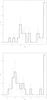 |
Fig. 1 Top panel: the distribution of F2 values (see text and Eq. (2)) for the combined sample of O and Y stars, by adopting an uncertainty of 88 m/s on every measurement. The dashed line is a reduced Gaussian distribution (mean of 0 and standard deviation of 1). Bottom panel: same as top, adopting an uncertainty of 220 m/s on every measurement. The dashed line is a Gaussian distribution of mean −2 and unit standard deviation. |
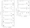 |
Fig. 2 Radial-velocity curves for the stars flagged as binaries (left column: Y stars; right column: O stars). The labels in each panel give the star number, σ(Vr) value (in km s-1), and probability of being a binary. |
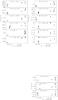 |
Fig. 3 Same as Fig. 2 for stars with no firm evidence for orbital motion. For most of these stars, a change in the zero-point offset by only 0.1 km s-1 (as compared to the value 0.42 ± 0.08 km s-1 used here) would considerably alter the visual impression of the existence or not of a long-term trend between the APOGEE and HERMES data. |
The value σ = 90 m/s appears to yield a F2 distribution adequately represented by a normal distribution with zero mean and unit standard deviation (see upper panel of Fig. 1). This value agrees well within the uncertainties of the HERMES and APOGEE measurements (Sect. 2.2). It also means that no jitter is expected to be present, since the measurement uncertainty suffices to adequately match the distribution of errors. The tail of large F2 values in Fig. 1 cannot be explained by the error distribution, or by an inadequate zero-point offset between the APOGEE and HERMES data. These stars are our best binary candidates.
We stressed in Sect. 2.2 that there is an uncertainty of 79 m/s due to zero point offset, which is comparable to the measurement uncertainty explained above. To be conservative and to allow for a possible error on the zero-point offset, not all stars in the large-F2 tail should be flagged as definite binaries. Therefore, the above process has been repeated, yet adopting this time a larger σ of 220 m/s. Although the normal distribution has a negative mean in this case (see bottom panel of Fig. 1) we found that this value allows us to recognise and set aside with better confidence those stars for which velocity variations may be due to either binarity or to an error on the zero-point offset (discussed in more detail below).
3.1.2. Binary probability
To be more quantitative, the probability Prob of the star being binary was calculated from the χ2 distribution considering N−1 degrees of freedom and σ = 220 m/s in Eq. (1) (see also Lucatello et al. 2005, for details). These values, together with the averaged RV and its standard deviation, are listed in Table 1. The full time span of the measurements is indicated in the last column of Table 1, showing that we deal with time spans of more than 1400 days for all stars.
Stars with 100% confidence of being binaries (Prob = 1) correspond toO1, O3, Y4, Y6, Y7, Y8, O8, Y9, O10, and Y12. Their radial-velocity curves are shown in Fig. 2. We may add Y2 in the figure: despite the fact that the confidence level of Y2 being a binary is only 56% (just below the 1σ confidence level); the HERMES measurements alone show a clear trend with an amplitude of 0.6 km s-1, which is well above the HERMES uncertainty of 0.22 km s-1.
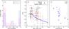 |
Fig. 4 Panel A) distribution of stars as a function of binary probability. There are more Y stars with high probabilities of being binaries than O stars. Panel B) [C/N] abundances as a function of mass for our sample of stars. The vertical dashed line marks the mass threshold between O and Y stars. Red symbols denote stars with probabilities larger than 68% of being binaries, while black symbols denote stars more likely to be single. The blue solid line indicates the theoretical relation between [12C/14N] and stellar mass in a post-FDU population, from Lagarde et al. (2012). There is no significant relation between [C/N] and binarity in the sample and several Y stars do not follow the theoretical relation. Panel C) [C/N] abundances as a function of surface gravity. Blue circles correspond to the Y stars and pink triangles represent O stars. |
The rest of the stars show no evidence of being binaries so far. Their radial-velocity curves are shown in Fig. 3. This conclusion is, however, somewhat dependent upon the adopted value of the zero-point offset. Some stars show a long-term trend (e.g. Y10, Y11, and Y13) , but their amplitude is not much larger than the uncertainty on the zero-point offset, so that no firm conclusion can be drawn at this stage. More HERMES observations are planned for the future to reach a definite conclusion about the binary nature of the stars depicted in Fig. 3. In summary, 54% of the sample of Y stars represents stars likely to be part of binary systems, as compared to 31% for the O stars. In panel A of Fig. 4, we show the binary probability distribution of the Y and O samples, plotted with blue and pink colours, respectively.
Since this result is based on a small sample with few measurements, it is worth evaluating whether or not this difference of binary frequencies between Y and O stars is statistically significant. To do so, we use the hypergeometric test as in Frankowski et al. (2009). We define Ny = No = 13 for the number of Y and O stars, and Nt = Ny + No = 26 for the total number of stars.Among these, we have xy = 7Y binaries, and xo = 4O binaries. We further define xt = xy + xo = 11. The frequency of binaries is then py = xy/Ny = 0.54, po = xo/No = 0.31 for the Y and the O samples, respectively, and pt = 0.42 for the total sample. The expected number of binaries in the Y sample ( ) is computed from the total fraction of binaries applied to the number of Y stars (
 ). The corresponding standard deviation on that inference (σxy) can be computed from the hypergeometric distribution given the total number of stars, the number of binaries and the number of Y stars: σxy = [Nypt(1−pt)(Nt−Ny)/(Ny−1)] 1/2 = 1.85. Finally, the significance of the difference between the expected and the observed binary frequencies
 ![Mathematical equation: \hbox{$(c^2 = [(\tilde{x_y} - x_y)/\sigma_{x_y}]^2 = 0.69)$}](/articles/aa/full_html/2016/11/aa29356-16/aa29356-16-eq91.png) may be computed from the χ2 distribution with one degree of freedom (see Frankowski et al. 2009, for details), which in this case corresponds to40%. Thus, given our data, there is a40% chance that the observed difference between the binary frequencies in the O and Y samples is simply due to statistical fluctuations.Admittedly, the significance of the existence of a true difference between the Y and O populations is not high yet.In the remainder of this article, we will nevertheless assume that the binary frequencies are truly different in the O and Y samples, with the fraction of Y binaries larger than the one of O binaries. This conclusion is supported by the fact that the percentage of 54% binaries found in the Y sample is especially large when compared to that found among comparison samples of K or M giants, where the percentage of spectroscopic binaries (observed under similar conditions as the Y and O samples discussed here) ranges between 6.3% and 30%, depending on the selection criterion of the sample (see the discussion by Frankowski et al. 2009). It may therefore be suspected that the large fraction of binaries (54%) among the Y sample is related to mass-transfer episodes responsible for the masses of Y stars, whereas the binary frequency among the O sample is similar to the upper range found among K giants.
may be computed from the χ2 distribution with one degree of freedom (see Frankowski et al. 2009, for details), which in this case corresponds to40%. Thus, given our data, there is a40% chance that the observed difference between the binary frequencies in the O and Y samples is simply due to statistical fluctuations.Admittedly, the significance of the existence of a true difference between the Y and O populations is not high yet.In the remainder of this article, we will nevertheless assume that the binary frequencies are truly different in the O and Y samples, with the fraction of Y binaries larger than the one of O binaries. This conclusion is supported by the fact that the percentage of 54% binaries found in the Y sample is especially large when compared to that found among comparison samples of K or M giants, where the percentage of spectroscopic binaries (observed under similar conditions as the Y and O samples discussed here) ranges between 6.3% and 30%, depending on the selection criterion of the sample (see the discussion by Frankowski et al. 2009). It may therefore be suspected that the large fraction of binaries (54%) among the Y sample is related to mass-transfer episodes responsible for the masses of Y stars, whereas the binary frequency among the O sample is similar to the upper range found among K giants.
It is important to remark that it is also possible that the larger frequency of RV variations among the Y sample as compared to the O sample could be due to differences in jitter related to mass. A definite answer on that question should await the demonstration of the Keplerian nature of the velocity variations for Y stars, even though the long-term trends already visible in Fig. 2 are clearly in favour of orbital variations.
3.2. Carbon and nitrogen
As shown by Masseron & Gilmore (2015), the [C/N] ratio in the APOGEE giants can be used as an indication of their mass. The first dredge-up (FDU) mixes material from the CN-processed inner layers to the surface of the star, at an amount that is a function of the stellar main-sequence mass (Iben 1965). Thus, [C/N] anticorrelates with mass in a post-FDU population (Lagarde et al. 2012; Tautvaišienė et al. 2015; Salaris et al. 2015; Martig et al. 2016).
We can check this correlation in the present sample, for which asteroseismic masses are available. Panel B of Fig. 4 shows our [C/N] ratio determinations as a function of stellar mass, indicating stars with Prob = 1 (presumably binaries) with red diamonds, and stars with Prob< 1 (presumably single stars) with black asterisks. The vertical dashed line represents the mass threshold used to define the O sample (masses below 1.2 M⊙ ,allowing for a 1σ error bar). The blue solid line corresponds to the theoretical relation of Lagarde et al. (2012) for the post-FDU models with Z = 0.004. To mimic the enhanced initial composition in [C/N] at low metallicity (Masseron & Gilmore 2015), we added 0.1 dex to the model predictions. We plot this relation to qualitatively show the expected anti-correlation of [C/N] vs. mass for single star, post-FDU models.
Many binary stars in panel B of Fig. 4 are clearly off this ([C/N], mass) anti-correlation, which therefore does not seem to apply for young α-rich stars (the Y sample). But since young α-rich stars are believed to be binaries, single star evolution models might not be relevant for them.
Moreover, as stated above, the [C/N] ratio should depend not only on mass, but also on the FDU occurrence. To distinguish pre-FDU stars from post-FDU stars, we plot in panel C of Fig. 4 the [C/N] ratio as a function of the surface gravity. In the models of Lagarde et al. (2012), the DUP tends to happen at approximately log g 3 (see lower panel of Fig. 1 of Masseron & Gilmore 2015, for different masses and metallicities), which is consistent with Panel C of Fig. 4, where the stars show a change in [C/N] of approximately log g of 2.5.
Therefore, if all stars with log g< 2.5 are indeed post-FDU objects, the fact that among those, Y stars have lower [C/N] ratio than O stars might, at first sight, seem puzzling in the framework of a mass transfer scenario. Indeed, Y stars are believed to have accreted [C/N] matter, in the past, from an O star. Accounting for dilution, the [C/N] ratio of any Y star could not be lower than the lowest [C/N] ratio observed for O stars. In fact, population synthesis simulations (see next section) show that the mass transfer is likely to occur during the Hertzsprung gap, before the FDU, thus polluting the companion with pristine gas, with [C/N] ~ 0. The decrease of the [C/N] ratio only occurs when the accretor itself experiences its FDU. Since the polluted star (Y) had, as a result of mass transfer, a larger main-sequence mass, its FDU is expected to more significantly decrease its [C/N] than it does for stars from the O sample. It is therefore not surprising that post-FDU stars from the Y sample tend to have lower [C/N] values than stars from the O sample of similar gravity, as illustrated in panel C of Fig. 4.
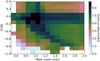 |
Fig. 5 [C/N] vs. mass in giant stars of our synthetic population by Izzard et al. (2004, 2006, 2009, in prep.) including initially 50% of binary stars and mass transfer via RLOF and wind-RLOF. The population has Z = 0.004 with all stars being older than 4 Gyr. |
3.3. Theoretical predictions from a population synthesis model
Since the previous section hints at binary systems playing a role in the occurrence of the Y population, we evaluated how binary interaction could account for increasing masses and altering binary orbits and surface abundances for the giant stars of the Y sample.
The population synthesis model used here follows the description of Izzard et al. (2004, 2006, 2009, and in prep.). We simulate a stellar population with 50% binary and 50% single stars, with a period distribution according to Duquennoy & Mayor (1991) and a flat mass-ratio distribution. We would add here that this frequency of 50% binaries is only to include binaries in our sample and adopting another value does not change our conclusions. The main idea here is to show that if we do not include binaries, there will be no mechanism to obtain massive stars. The amount of resulting massive stars from the binary evolution depends on the fraction of initial binaries and single stars, as well as the period distributions of the binaries. This is discussed in depth in a complementary article on this subject (Izzard et al., in prep.). Mass transfer in binaries follows the Roche Lobe overflow formulation (RLOF) of Claeys et al. (2014), which depends on the mass ratio of the binary system q. Wind mass transfer is based on the wind-RLOF formalism of Abate et al. (2013, 2015). Our synthetic population has a metallicity of Z = 0.004, which is consistent with the thick disk population. Because our goal is to test whether mass transfer can produce 1.4 M⊙ stars in the thick disk, our population contains only stars older than 4 Gyr, corresponding to single stars with masses below 1.2 M⊙. A study complementary to this current one discusses in depth the different input physics of this model and how the model results compare to the observations of the APOKASC sample (Izzard et al., in prep.). Here we only focus on a qualitative comparison, showing that interacting binaries can also explain the characteristics seen in the stars of the Y sample.
In Fig. 5 we plot [C/N] as a function of mass in our synthetic population using the colour scheme of Green (2011). The shading indicates the logarithm of the number of stars in a given [C/N]-mass bin. The first interesting aspect to note is that, while we did not allow for single stars with M> 1.2 M⊙ in the initial sample; binary interaction creates stars with masses above this value. Furthermore, the model reproduces the standardanticorrelation between [C/N] and mass (similar to that for single stars from Lagarde et al. 2012, shown in Fig. 4). It predicts a secondary sequence at constant [C/N]. As discussed above, the latter is not predicted in a single stellar evolution scenario.
Some model stars have masses ~ 1 M⊙ and high [C/N] in Fig. 5. This is the locus occupied by post-mass-transfer giants in binary systems like CH, barium and extrinsic S stars (Keenan 1942; Bidelman & Keenan 1951; McClure & Woodsworth 1990; Jorissen et al. 1998; Izzard et al. 2004, 2009). They are products of wind mass transfer from an AGB donor which was able to synthesise C and s-process elements. Since those stars are not present in our observed sample, we will not discuss them further here (but it is definitely worth searching for them in the APOKASC sample).
3.4. Discussion
Stars with M> 1.4 M⊙ found in the thick disk by Kepler and CoRoT have been interpreted as young stars. This challenges Galactic evolution models because it is not easy to explain the presence of such young, α-enhanced stars in the solar neighbourhood (Minchev et al. 2013). One explanation is that they were formed in the region near the co-rotating bar, which is where the gas can be kept inert for a long time and expelled to outer regions by radial migration (Minchev et al. 2014; Chiappini et al. 2015). It is still not clear how to make the young α-rich stars migrate from the bar to the solar vicinity in the lifetime of such young stars. It is worth noting that Cantat-Gaudin et al. (2014) and Magrini et al. (2015) discuss the nature of the young α-rich open cluster NGC 6705(of age 0.30 ± 0.05 Gyr and with [Mg/Fe] ~ [Si/Fe] ~ + 0.3 dex for [Fe/H] = + 0.10 ± 0.06 dex, based on the analysis of 21 stars). This cluster is more metal-rich than the stars analysed here and these authors propose that the α-enrichment of this young cluster might be due to local enrichment of the molecular cloud from supernova explosions, instead of radial migration.
In this article we discuss whether binary stars could account for the (sub)giant stars dubbed “young α-rich”. We propose that they were blue straggler main-sequence stars or other binary stars that underwent mass-transfer in the past. This agrees with a recent suggestion by Brogaard et al. (2016) based on a work on open clusters with eclipsing binary systems and asteroseismic observations. It is also in agreement with the recent study by Tayar et al. (2015), who analysed anomalous rotational velocities in APOKASC and explained them as mass transfer products.
The Y stars could have been formed following a mass-transfer scenario, as for other BSSs found in the field (McCrea 1964; Preston 2015). Since BSSs have orbital periods which cluster around 103 d (Geller & Mathieu 2012), a time span longer than the few days spanned by the data used by Martig et al. (2015) is required to assess their binary nature. Indeed, with observations spanning more than 1000 days, we already find more than 50% of binaries among the Y sample. More should be expected with an even longer time span.
Our results support the following formation scenario for the stars belonging to the Y sample: when the less massive component of the system is still on the main sequence, it accretes matter from its more massive companion donor star as the latter evolves through the Hertzsprung gap. Since this phase corresponds to a rapid increase of the stellar radius, for close-enough systems, RLOF will occur. In this phase, the system may look like an Algol (once the mass ratio has been reversed), and a substantial amount of mass may be transferred from the donor to the accretor. Because the Hertzsprung gap happens before FDU, the donor transfers pristine gas, that is, with [C/N] ~ 0. Thus, as the accretor gains mass, it moves horizontally to the right in Fig. 5. At the same time, in the Hertzsprung-Russell diagram the accretor becomes a blue straggler. Long after mass transfer has ceased, the accretor itself leaves the main sequence to become a red giant. Before FDU, the giant preserves its pristine [C/N] ~ 0. After FDU, [C/N] decreases by the amount fixed by its current mass, as seen for single stars, thus moving downwards to the blue sequence of panel B in Fig. 4, equivalent to the lower sequence seen in Fig. 5.
Lithium is another element that depletes after FDU. It is thus possible that some stars with [C/N] ~ 0 (pre-FDU) are also Li-normal. The chemical abundance analysis of Jofré et al. (2015a) showed that the star Y1 is Li-enhanced to normal (A(Li) = 1.8). If we assume (i) the abundance of Li of Y1 is pristine for a pre-FDU star, and (ii) Y1 is not a binary star, then Y1 could be one of the truly young α-rich stars proposed by Martig et al. (2015) and Chiappini et al. (2015). Y1 could also be a merger product such as those suggested by Tayar et al. (2015), although in this case the star should have lost angular momentum as its rotational velocity is low (vsini ~ 1 km s-1, Jofré et al. 2015a). That said, it has been suggested that mass transfer in blue stragglers should, rather, destroy Li (Carney et al. 2005), although the picture is not so simple since other mass-transfer products show a large scatter in Li abundance, from Li-depleted to Li-rich (see e.g. discussions in Masseron et al. 2012; Hansen et al. 2016).
4. Conclusions
In this article we have shown that binary stars may also explain the nature of young α-rich stars. Our observations reveal that the sample used by Martig et al. (2015) to show that these stars are young contains a substantial percentage of binaries (at least 50%), and therefore isochrones of individual objects should not be used for determining the age of these stars. In addition, our population synthesis model shows that it is possible to obtain the (high) masses and [C/N] abundances of these stars by mass-transfer in binary systems. A more detailed population synthesis study focusing in a more quantitative way on the binary fraction and mass distribution of the APOKASC sample is on-going (Izzard et al., in prep.). Furthermore,long-term monitoring of the RVs of our sample is still on-going, with the aim of obtaining accurate orbital properties even for long-period binaries.Parameters like the orbital eccentricity, and more generally the location of the systems in the eccentricity-period diagram, provide crucial help in understanding the process of mass transfer. RV monitoring takes time (Preston 2009) and therefore patience is the key ingredient needed to disentangle the origin of these interesting objects and finally quantify how many of them are truly young stars.
As Wheeler (1979) wrote, BSSs seem to be both inadequately understood and insufficiently appreciated. However, we know that as long as the possibility of mass transfer exists, blue stragglers will form. Because many show no evident signatures in their spectra(Yong et al. 2016)and because they might be the product of coalescence resulting in single objects, identifying those BSSs that have evolved off the main-sequence has so far been an almost impossible task. Spectro-seismic surveys give us a unique opportunity to study them, opening a new window to the physics of stellar evolution and mass transfer.
Acknowledgments
This work was partly supported by the European Union FP7 programme through ERC grant number 320360. P.J. acknowledges King’s College Cambridge for partially supporting this work. We thank C. Tout and S. Aarseth for discussion on the subject. K.H. is supported by Marshall Scholarship and King’s College Cambridge Studenship. R.J.I. thanks the STFC for funding his Rutherford Fellowship. Based on observations made with the Mercator Telescope, operated on the island of La Palma by the Flemish Community, at the Spanish Observatorio del Roque de los Muchachos of the Instituto de Astrofí sica de Canarias. Based on observations obtained with the HERMES spectrograph, which is supported by the Research Foundation – Flanders (FWO), Belgium, the Research Council of KU Leuven, Belgium, the Fonds National de la Recherche Scientifique (F.R.S. – FNRS), Belgium, the Royal Observatory of Belgium, the Observatoire de Genève, Switzerland and the Thüringer Landessternwarte Tautenburg, Germany.
References
- Abate, C., Pols, O. R., Izzard, R. G., Mohamed, S. S., & de Mink, S. E. 2013, A&A, 552, A26 [NASA ADS] [CrossRef] [EDP Sciences] [Google Scholar]
- Abate, C., Pols, O. R., Stancliffe, R. J., et al. 2015, A&A, 581, A62 [NASA ADS] [CrossRef] [EDP Sciences] [Google Scholar]
- Anders, F., Chiappini, C., Santiago, B. X., et al. 2014, A&A, 564, A115 [NASA ADS] [CrossRef] [EDP Sciences] [Google Scholar]
- Baglin, A., Auvergne, M., Boisnard, L., et al. 2006, in 36th COSPAR Scientific Assembly [Google Scholar]
- Bidelman, W. P., & Keenan, P. C. 1951, ApJ, 114, 473 [NASA ADS] [CrossRef] [Google Scholar]
- Boffin, H. M. J., Carraro, G., & Beccari, G. 2015, Ecology of Blue Straggler Stars [Google Scholar]
- Borucki, W. J., Koch, D., Basri, G., et al. 2010, Science, 327, 977 [NASA ADS] [CrossRef] [PubMed] [Google Scholar]
- Brogaard, K., Jessen-Hansen, J., Handberg, R., et al. 2016, Astron. Nachr., 337, 793 [NASA ADS] [CrossRef] [Google Scholar]
- Cantat-Gaudin, T., Vallenari, A., Zaggia, S., et al. 2014, A&A, 569, A17 [NASA ADS] [CrossRef] [EDP Sciences] [Google Scholar]
- Carney, B. W., Latham, D. W., Laird, J. B., Grant, C. E., & Morse, J. A. 2001, AJ, 122, 3419 [NASA ADS] [CrossRef] [Google Scholar]
- Carney, B. W., Latham, D. W., & Laird, J. B. 2005, AJ, 129, 466 [NASA ADS] [CrossRef] [Google Scholar]
- Carney, B. W., Latham, D. W., Stefanik, R. P., & Laird, J. B. 2008, AJ, 135, 196 [NASA ADS] [CrossRef] [Google Scholar]
- Chaplin, W. J., Kjeldsen, H., Christensen-Dalsgaard, J., et al. 2011, Science, 332, 213 [NASA ADS] [CrossRef] [PubMed] [Google Scholar]
- Chen, X., & Han, Z. 2008a, MNRAS, 384, 1263 [NASA ADS] [CrossRef] [Google Scholar]
- Chen, X., & Han, Z. 2008b, MNRAS, 387, 1416 [NASA ADS] [CrossRef] [Google Scholar]
- Chiappini, C., Anders, F., Rodrigues, T. S., et al. 2015, A&A, 576, L12 [NASA ADS] [CrossRef] [EDP Sciences] [Google Scholar]
- Chubak, C., Marcy, G., Fischer, D. A., et al. 2012, ArXiv e-prints [arXiv:1207.6212] [Google Scholar]
- Claeys, J. S. W., Pols, O. R., Izzard, R. G., Vink, J., & Verbunt, F. W. M. 2014, A&A, 563, A83 [NASA ADS] [CrossRef] [EDP Sciences] [Google Scholar]
- Duquennoy, A., & Mayor, M. 1991, A&A, 248, 485 [NASA ADS] [Google Scholar]
- Eisenstein, D. J., Weinberg, D. H., Agol, E., et al. 2011, AJ, 142, 72 [Google Scholar]
- Famaey, B., Pourbaix, D., Frankowski, A., et al. 2009, A&A, 498, 627 [NASA ADS] [CrossRef] [EDP Sciences] [Google Scholar]
- Frankowski, A., Famaey, B., van Eck, S., et al. 2009, A&A, 498, 479 [NASA ADS] [CrossRef] [EDP Sciences] [Google Scholar]
- Geller, A. M., & Mathieu, R. D. 2012, AJ, 144, 54 [NASA ADS] [CrossRef] [Google Scholar]
- Green, D. A. 2011, Bull. Astron. Soc. India, 39, 289 [Google Scholar]
- Hansen, C. J., Jofré, P., Koch, A., et al. 2016, A&A, submitted [Google Scholar]
- Hawkins, K., Masseron, T., Jofre, P., et al. 2016, A&A, 594, A43 [NASA ADS] [CrossRef] [EDP Sciences] [Google Scholar]
- Haywood, M., Di Matteo, P., Lehnert, M. D., Katz, D., & Gómez, A. 2013, A&A, 560, A109 [NASA ADS] [CrossRef] [EDP Sciences] [Google Scholar]
- Holtzman, J. A., Shetrone, M., Johnson, J. A., et al. 2015, AJ, 150, 148 [NASA ADS] [CrossRef] [Google Scholar]
- Iben, Jr., I. 1965, ApJ, 142, 1447 [NASA ADS] [CrossRef] [Google Scholar]
- Izzard, R. G., Tout, C. A., Karakas, A. I., & Pols, O. R. 2004, MNRAS, 350, 407 [NASA ADS] [CrossRef] [Google Scholar]
- Izzard, R. G., Dray, L. M., Karakas, A. I., Lugaro, M., & Tout, C. A. 2006, A&A, 460, 565 [NASA ADS] [CrossRef] [EDP Sciences] [Google Scholar]
- Izzard, R. G., Glebbeek, E., Stancliffe, R. J., & Pols, O. R. 2009, A&A, 508, 1359 [NASA ADS] [CrossRef] [EDP Sciences] [Google Scholar]
- Jofré, P., & Weiss, A. 2011, A&A, 533, A59 [NASA ADS] [CrossRef] [EDP Sciences] [Google Scholar]
- Jofré, P., Heiter, U., Soubiran, C., et al. 2014, A&A, 564, A133 [NASA ADS] [CrossRef] [EDP Sciences] [Google Scholar]
- Jofré, E., Petrucci, R., García, L., & Gómez, M. 2015a, A&A, 584, L3 [NASA ADS] [CrossRef] [EDP Sciences] [Google Scholar]
- Jofré, P., Heiter, U., Soubiran, C., et al. 2015b, A&A, 582, A81 [NASA ADS] [CrossRef] [EDP Sciences] [Google Scholar]
- Jorissen, A., & Mayor, M. 1988, A&A, 198, 187 [NASA ADS] [Google Scholar]
- Jorissen, A., Van Eck, S., Mayor, M., & Udry, S. 1998, A&A, 332, 877 [NASA ADS] [Google Scholar]
- Jorissen, A., Van Eck, S., Van Winckel, H., et al. 2016, A&A, 586, A158 [NASA ADS] [CrossRef] [EDP Sciences] [Google Scholar]
- Keenan, P. C. 1942, ApJ, 96, 101 [NASA ADS] [CrossRef] [Google Scholar]
- Lagarde, N., Decressin, T., Charbonnel, C., et al. 2012, A&A, 543, A108 [NASA ADS] [CrossRef] [EDP Sciences] [Google Scholar]
- Lucatello, S., Tsangarides, S., Beers, T. C., et al. 2005, ApJ, 625, 825 [NASA ADS] [CrossRef] [Google Scholar]
- Magrini, L., Randich, S., Donati, P., et al. 2015, A&A, 580, A85 [NASA ADS] [CrossRef] [EDP Sciences] [Google Scholar]
- Martig, M., Rix, H.-W., Aguirre, V. S., et al. 2015, MNRAS, 451, 2230 [NASA ADS] [CrossRef] [Google Scholar]
- Martig, M., Fouesneau, M., Rix, H.-W., et al. 2016, MNRAS, 456, 3655 [NASA ADS] [CrossRef] [Google Scholar]
- Masseron, T., & Gilmore, G. 2015, MNRAS, 453, 1855 [NASA ADS] [CrossRef] [Google Scholar]
- Masseron, T., Johnson, J. A., Lucatello, S., et al. 2012, ApJ, 751, 14 [NASA ADS] [CrossRef] [Google Scholar]
- McClure, R. D., & Woodsworth, A. W. 1990, ApJ, 352, 709 [NASA ADS] [CrossRef] [Google Scholar]
- McCrea, W. H. 1964, MNRAS, 128, 147 [NASA ADS] [CrossRef] [Google Scholar]
- Minchev, I., Chiappini, C., & Martig, M. 2013, A&A, 558, A9 [NASA ADS] [CrossRef] [EDP Sciences] [Google Scholar]
- Minchev, I., Chiappini, C., Martig, M., et al. 2014, ApJ, 781, L20 [NASA ADS] [CrossRef] [Google Scholar]
- Nidever, D. L., Holtzman, J. A., Allen de Prieto, C., et al. 2015, AJ, 150, 173 [NASA ADS] [CrossRef] [Google Scholar]
- Pinsonneault, M. H., Elsworth, Y., Epstein, C., et al. 2014, ApJS, 215, 19 [NASA ADS] [CrossRef] [Google Scholar]
- Piotto, G., De Angeli, F., King, I. R., et al. 2004, ApJ, 604, L109 [NASA ADS] [CrossRef] [Google Scholar]
- Preston, G. W. 2009, PASA, 26, 372 [NASA ADS] [CrossRef] [Google Scholar]
- Preston, G. W. 2015, Field Blue Stragglers and Related Mass Transfer Issues, eds. H. M. J. Boffin, G. Carraro, & G. Beccari, 65 [Google Scholar]
- Preston, G. W., & Sneden, C. 2000, AJ, 120, 1014 [NASA ADS] [CrossRef] [Google Scholar]
- Raskin, G., van Winckel, H., Hensberge, H., et al. 2011, A&A, 526, A69 [NASA ADS] [CrossRef] [EDP Sciences] [Google Scholar]
- Salaris, M., Pietrinferni, A., Piersimoni, A. M., & Cassisi, S. 2015, A&A, 583, A87 [NASA ADS] [CrossRef] [EDP Sciences] [Google Scholar]
- Sandage, A. R. 1953, AJ, 58, 61 [NASA ADS] [CrossRef] [Google Scholar]
- Santucci, R. M., Placco, V. M., Rossi, S., et al. 2015, ApJ, 801, 116 [NASA ADS] [CrossRef] [Google Scholar]
- Setiawan, J., Pasquini, L., da Silva, L., von der Lühe, O., & Hatzes, A. 2003, A&A, 397, 1151 [NASA ADS] [CrossRef] [EDP Sciences] [Google Scholar]
- Tautvaišienė, G., Drazdauskas, A., Mikolaitis, Š., et al. 2015, A&A, 573, A55 [NASA ADS] [CrossRef] [EDP Sciences] [Google Scholar]
- Tayar, J., Ceillier, T., García-Hernández, D. A., et al. 2015, ApJ, 807, 82 [NASA ADS] [CrossRef] [Google Scholar]
- Udry, S., Mayor, M., & Queloz, D. 1999, in Precise Stellar Radial Velocities IAU Colloq. 170, eds. J. B. Hearnshaw, & C. D. Scarfe, ASP Conf. Ser., 185, 367 [Google Scholar]
- Unavane, M., Wyse, R. F. G., & Gilmore, G. 1996, MNRAS, 278, 727 [NASA ADS] [CrossRef] [Google Scholar]
- Wheeler, J. C. 1979, ApJ, 234, 569 [Google Scholar]
- Wilson, E. B., & Hilferty, M. M. 1931, Proc. Natl. Acad. Sci., 17, 684 [NASA ADS] [CrossRef] [Google Scholar]
- Yong, D., Casagrande, L., Venn, K. A., et al. 2016, MNRAS, 459, 487 [NASA ADS] [CrossRef] [Google Scholar]
Appendix A: Individual radial velocity measurements
In this appendix we list the radial velocities we used for the analysis presented in this work. The values obtained in 2011 and 2012 are taken from the individual visits APOGEE Survey and the RVs have been determined by Nidever et al. (2015). The values obtained in 2015 and 2016 were taken from HERMES observations, and have been determined by us. Table A.1 has two main columns; the left-hand column shows the RVs of the Y stars while the right-hand column shows the RVs for the O stars. Note that every star has at least three independent observations, allowing us to distinguish between an erroneous measurement and a possible binary.
Radial velocity measurements for individual epochs.
All Tables
All Figures
|
Fig. 1 Top panel: the distribution of F2 values (see text and Eq. (2)) for the combined sample of O and Y stars, by adopting an uncertainty of 88 m/s on every measurement. The dashed line is a reduced Gaussian distribution (mean of 0 and standard deviation of 1). Bottom panel: same as top, adopting an uncertainty of 220 m/s on every measurement. The dashed line is a Gaussian distribution of mean −2 and unit standard deviation. |
| In the text | |
|
Fig. 2 Radial-velocity curves for the stars flagged as binaries (left column: Y stars; right column: O stars). The labels in each panel give the star number, σ(Vr) value (in km s-1), and probability of being a binary. |
| In the text | |
|
Fig. 3 Same as Fig. 2 for stars with no firm evidence for orbital motion. For most of these stars, a change in the zero-point offset by only 0.1 km s-1 (as compared to the value 0.42 ± 0.08 km s-1 used here) would considerably alter the visual impression of the existence or not of a long-term trend between the APOGEE and HERMES data. |
| In the text | |
|
Fig. 4 Panel A) distribution of stars as a function of binary probability. There are more Y stars with high probabilities of being binaries than O stars. Panel B) [C/N] abundances as a function of mass for our sample of stars. The vertical dashed line marks the mass threshold between O and Y stars. Red symbols denote stars with probabilities larger than 68% of being binaries, while black symbols denote stars more likely to be single. The blue solid line indicates the theoretical relation between [12C/14N] and stellar mass in a post-FDU population, from Lagarde et al. (2012). There is no significant relation between [C/N] and binarity in the sample and several Y stars do not follow the theoretical relation. Panel C) [C/N] abundances as a function of surface gravity. Blue circles correspond to the Y stars and pink triangles represent O stars. |
| In the text | |
|
Fig. 5 [C/N] vs. mass in giant stars of our synthetic population by Izzard et al. (2004, 2006, 2009, in prep.) including initially 50% of binary stars and mass transfer via RLOF and wind-RLOF. The population has Z = 0.004 with all stars being older than 4 Gyr. |
| In the text | |
Current usage metrics show cumulative count of Article Views (full-text article views including HTML views, PDF and ePub downloads, according to the available data) and Abstracts Views on Vision4Press platform.
Data correspond to usage on the plateform after 2015. The current usage metrics is available 48-96 hours after online publication and is updated daily on week days.
Initial download of the metrics may take a while.