| Issue |
A&A
Volume 595, November 2016
|
|
|---|---|---|
| Article Number | A104 | |
| Number of page(s) | 10 | |
| Section | The Sun | |
| DOI | https://doi.org/10.1051/0004-6361/201629000 | |
| Published online | 08 November 2016 | |
Sunspot positions, areas, and group tilt angles for 1611−1631 from observations by Christoph Scheiner⋆
1 Leibniz-Institut für Astrophysik Potsdam (AIP), An der Sternwarte 16, 14482 Potsdam, Germany
e-mail: This email address is being protected from spambots. You need JavaScript enabled to view it.
2 Institut für Physik und Astronomie, Universität Potsdam, Karl-Liebknecht-Str. 24/25, 14476 Potsdam, Germany
Received: 25 May 2016
Accepted: 5 August 2016
Abstract
Aims. Digital images of observations printed in the books Rosa Ursina sive solis and Prodromus pro sole mobili by Christoph Scheiner, as well as the drawings from Scheiner’s letters to Marcus Welser, are analysed to obtain information on the positions and sizes of sunspots that appeared before the Maunder minimum.
Methods. In most cases, the given orientation of the ecliptic is used to set up the heliographic coordinate system for the drawings. Positions and sizes are measured manually on screen. Very early drawings have no indication of their orientation. A rotational matching using common spots of adjacent days is used in some cases, while in other cases, the assumption that images were aligned with a zenith-horizon coordinate system appeared to be the most probable.
Results. In total, 8167 sunspots were measured. A distribution of sunspot latitudes versus time (butterfly diagram) is obtained for Scheiner’s observations. The observations of 1611 are very inaccurate, the drawings of 1612 have at least an indication of their orientation, while the remaining part of the spot positions from 1618−1631 have good to very good accuracy. We also computed 697 tilt angles of apparently bipolar sunspot groups observed in the period 1618−1631. We find that the average tilt angle of nearly 4 degrees is not significantly different from 20th-century values.
Key words: Sun: activity / sunspots / history and philosophy of astronomy
Data on the sunspot position and area are only available at the CDS via anonymous ftp to cdsarc.u-strasbg.fr (130.79.128.5) or via http://cdsarc.u-strasbg.fr/viz-bin/qcat?J/A+A/595/A104
© ESO, 2016
1. Introduction
Solar activity is to a large extent characterized by the sunspot number and the latitudinal distribution of spots as functions of time. More information on the activity is, of course, accessible if enough details of the structures at the solar surface are available.
Extending the sunspot record back in time is not only a matter of obtaining reliable sunspot numbers and related indices for as many cycles as possible, but it is also a matter of reconstructing the solar butterfly diagram of the Sun. With the available sources of pre-photographic observations, we may be able to compile an almost complete butterfly diagram for the telescopic era since AD 1610.
Not many publications exist with positional measurements of sunspots observed in the beginning of this era, namely in the first half of the 17th century. Studies of the solar rotation are available for Harriot by Herr (1978) for the period 1611−1613, for Scheiner by Eddy et al. (1977) for the period 1625−1626, for Hevelius by Eddy et al. (1976) and Abarbanell & Wöhl (1981) for 1642−1644, and for Scheiner as well as Hevelius by Yallop et al. (1982), but the sunspot positions were not published. Sunspot positions from Galileo’s observations in 1612 were derived and made available by Casas et al. (2006)1.
Christoph Scheiner lived from 1573−1650 (Braunmühl 1891; Hockey et al. 2007)2 and was a member of the Jesuit society (Societas Iesu). The present paper is based on the copy of Scheiner (1630) stored in the library of the Leibniz Institute for Astrophysics Potsdam (AIP) and Scheiner (1651) at the library of ETH Zürich, available as a high-resolution digital version through the Swiss platform for digitized content, e-rara3. The observations cover the years of 1611−1631, albeit most of the data comes from 1625 and 1626. Data from the period before the Maunder minimum are interesting since they may tell us details about how the Sun went into a low-activity phase that lasted for about five decades, in particular since Vaquero & Trigo (2015) suggested that the declining phase of the solar cycle had already started around 1618.
If information on individual sunspots and pores within sunspot groups is preserved, quantities such as the polarity separation and the tilt angle of bipolar groups may be inferred. It will be of particular interest to discover whether these quantities behaved differently in the period before the Maunder minimum as compared to the cycles after it or present cycles. This is not the first attempt to use sunspot positions derived from Scheiner’s observations. An estimate of the differential rotation was, for example, derived from Scheiner’s book by Eddy et al. (1977), who concluded that the rotation profile was not significantly different from the one obtained for the 20th century. The authors did not, however, publish the obtained spot positions. Scheiner actually noticed different rotation periods for different spots spanning from 25 d to 28 d (Scheiner 1630, p. 559). He does not, however, say that these periods were attached to specific latitudes of spots.
Scheiner (1573−1650) belongs − together with Johannes Fabricius, Galileo Galilei, Thomas Harriot, Joachim Jungius, Simon Marius, and Adam Tanner (Neuhäuser & Neuhäuser 2016) − to the first observers who left records of sunspots seen through a telescope. Scheiner’s first observations were made in early March 1611, together with the student Johann Baptist Cysat (1586−1657). Scheiner was the first observer to start sunspot drawings on a systematic, day-by-day basis in October 1611. A comprehensive investigation of the sunspot observations of the 1610s can be found in Neuhäuser & Neuhäuser (2016).
The following paper describes the drawings and gives details of the drawings in Sect. 2, explains the measuring method for 1618−1631 in Sect. 3, the methods used to utilize the drawings of 1611−1612 in Sect. 4, evaluates the accuracy of the data in Sect. 5, gives the data format and the butterfly diagram in Sect. 6, and deals with the sunspot group tilt angles in Sect. 7. A summary is given in Sect. 8.
2. Description of the Rosa Ursina and Prodromus drawings
Scheiner (1630) provides 71 main image plates with observations, of which one is unnumbered since it contains only detailed faculae drawings, plus an additional plate with his first observations of 1611. The plates always contain information on more than one day. The number of different days covered varies between four and 54. Early drawings are available from the letters of Scheiner to Marcus Welser in 1611 and 1612. Further sunspot drawings are printed in Scheiner (1651), where Scheiner defends the geocentric model. There are 12 image plates with spots from 1625, 1626, 1629, and 1631. The drawings are in exactly the same style as the ones in Scheiner (1630), and we used the same analysis procedure as described below. The total number of days for which we have sunspot information is 798, while two additional days show only faculae. Table 1 gives the annual numbers of days available.
Numbers of days available for given years as reported by Scheiner (1630), Scheiner (1651), and Reeves & Van Helden (2010).
Five observing locations contributed to this compilation of results on sunspots. Scheiner was located in Rome, Italy, in the years 1624−1633 and we assume geographical coordinates of  eastern longitude and
  northern latitude for his position. The other locations were Ingolstadt in Germany, Douai (Duacum in Latin) in France, Freiburg im Breisgau, Germany, and Vienna, Austria.
The University of Freiburg and the Jesuit church next to it were located at  E,
E,  N. One probable observer was a pupil of Scheiner, Georg Schönberger (or Schomberger) (Braunmühl 1891) who later observed with Johann Nikolaus Smogulecz (or Jan Mikołaj Smogulecki). The observations are also available in a separate publication by Smogulecz & Schönberger (1626).
For Ingolstadt, we assumed the position of the original university building, Hohe Schule, at  E and
E and  N. Scheiner gave the geographical latitude on top of a page of 1611 observations as
  . After Scheiner left Ingolstadt in 1616, the observers could have been Scheiner’s pupils, among them Johann Baptist Cysat, Chrysostomus Gall, and Georg Schönberger (Braunmühl 1891). Cysat taught in Luzern, Switzerland, from 1624−1627 though (Zinner 1957). Since the observations from Ingolstadt that were not made by Scheiner cover the period from 1623 March 26 to 1625 September 15, they were most likely not made by Cysat. Scheiner cites Georg Schönberger as the correspondent of the Ingolstadt observations, but Schönberger taught in Freiburg later, and his books of 1622 and 1626 were published in Freiburg. It remains unclear to us who was the observer in Ingolstadt.
For Douai, we assume approximately  E,
E,  N. Since the University of Douai was a conglomerate of colleges and the Jesuits erected their own school in the 1620s, it is less obvious from which exact place they observed, but not really relevant for the scope of this paper. The observer in Douai was Karel Malapert (Charles Malapert, Carolus Malapertius) who published his own observations in two books (Malapertius 1620, 1633). While it was published in Douai, Braunmühl (1891) mentions his observations to be made at Danzig, Poland. This may be a translation error of Duacum, although Malapert did teach in Poland, but at the Jesuit College of Kalisz from 1613−1617 (Birkenmajer 1967). Scheiner regularly compares the observations of the three sites in his figures. We include all spots visible in these drawings in the data set, but if a spot was observed by Scheiner as well as a colleague on the same day, we give only Scheiner’s spot position.
The location of the Jesuit church in Vienna is about  E,
E,  N. Scheiner names Johann Cysat as the observer whose life between 1627 and 1631 is not known in detail. At least, we find an indication that Cysat was in Vienna “occasionally” in that period from Zinner (1957). Scheiner compared the Vienna data with the Rome data, so there is eventually only a total of six spot measurements that complemented the Rome data (recorded on 1629 August 12, 13, and 20).
Typical figures contain a circle for the solar limb, a horizontal line mostly denoting the ecliptic, and a selected number of sunspot groups that are followed on several days. The dates (in many cases together with a precise time and the elevation of the Sun) are given in a small table within the circle.
The next figure gives another set of selected groups for a sequence of days. We note that these sequences of some drawings very often overlap. The figures are made in such a way as to show all appearances of a given group on as many days as necessary.
Times are given in 12-h format, annotated with “m” = matutinus = morning and “u” = uespera = vespera = evening. The only exception is the first drawing of the 1624−1631 spell. The times are all above 12:00, but since Scheiner also gave the elevations of the Sun, we can guess the most plausible meaning for the times. We find that the time was very likely measured from the last sunset, which is at about 16:25 local time in Rome in mid-December. The corresponding local times in today’s reading are given in Table 2, sorted by local time instead of date. All other plates give local times apparently measured from midnight.
Assumed times specially for Plate I.
The printed versions of the drawings were digitized with a book scanner at a resolution of 200 dpi. One pixel corresponds to 0.13 mm converting to an angular distance of a bit less than  in heliographic coordinates in the solar disk centre. The observations of 1611 December 14 to 1612 April 7 were not shown by Scheiner (1630); these were digitized from Reeves & Van Helden (2010). Their diameter is about 22.7 mm. A distance of 0.1 mm on those disks corresponds to an angle of
  in heliographic coordinates in the disk centre.
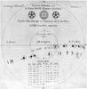 |
Fig. 1 Example of an early drawing, indicating the directions and an inner circle annotated as the observed circle. All spots appear twice: once in the inner circle and once in the full circle. |
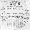 |
Fig. 2 Example of a variable ecliptic line to avoid crowdedness. Spots near the eastern and western limbs of the southern-hemisphere groups are rotated above and below their actual position for better visibility. Group a in the northern hemisphere is unaffected. |
The images I to V, IX, X, XVI, XVII contain a smaller circle which is annotated as the “circellus observatorius” = “observed circle”, while the large circle covering almost the entire page is entitled the “circulus ampliatus ex observatorio” = “circle expanded by observatory”. Figure 1 shows the example of Plate III. Spots are plotted twice in these drawings, once at the scale of the inner circle and once at the scale of the outer circle. We use the large version of the drawing for position and area measurements. As shown in Sect. 5, the accuracy of the positions is remarkable, even though the large images may be the result of post-observational magnifications.
Another peculiarity is shown in Fig. 2 covering the period of 1625 March 20 to April 6. The southern hemisphere of the Sun was so crowded with spots that some sunspot groups were plotted into a rotated coordinate system to avoid overlap with groups of other days. A few spots were actually plotted twice: once within the crowd of spots and once at another location. These spots indicate that it is indeed a rotation of the disk by multiples of roughly 15° that led to the secondary positions, and not a linear shift upward or downward.
Image XX contains a large number of faculae crossing the solar disk, while there is only a small group on the southern hemisphere for which we actually determined positions and sizes.
Image XXII shows extended faculae at the eastern limb and sunspots for the period 1625 May 2−14. The faculae of May 3 are drawn in a rather dark colour, possibly indicating very bright faculae, keeping in mind that faculae needed to be plotted with an inverse greyscale. There is a large c-shaped black area surrounding a blank-paper region which appears bright in contrast to the dark surrounding faculae. Rek (2010) seem to argue in a footnote that this region may have been a white-light flare. The textual description of 1625 May 2−4 by Scheiner (1630, p. 208) says the following: (While Scheiner uses the word “umbra”, we translated it into shadow, since the conception of an umbra may have been different to today’s definition.) Since there is no mention of a phenomenon being variable during the course of the day, there is no clear evidence for a white-light flare, despite the presence of a peculiar sunspot group.
There is an unnumbered image plate between images XXVI and XXVII that contains only faculae and covers days that were already shown in images XXIII and XXIV, and has therefore not been used in our measurements.
3. The coordinate system of the drawings of 1618−1631
Scheiner describes his observing method as a projection behind the telescope(s). This would mean that the appearance of the Sun was mirrored. There are several indications, however, that he made the actual images in a non-mirrored way, and the orientation of the drawings is roughly upright.
More precisely, the drawings always show a nearly horizontal line representing the ecliptic. Since the plane of the ecliptic is not easily accessible when observing under the sky, it has apparently been computed by Scheiner from the direction to the local zenith. The direction to the local zenith is marked on a few drawings by little dots at the solar limb.
We need to find the angle between the direction of the solar rotation axis and the pole of the ecliptic. As already performed by Arlt et al. (2013), we use the output of the angle of the solar rotation axis with the direction to the true-of-date celestial north pole, as provided by the JPL Horizons ephemeris webpage4. The ecliptic pole is assumed to be at αE = 18h,  , which is true-of-date by definition (neglecting orbital precession and nutation). We then use a spherical transformation to obtain the missing angle between the celestial north pole and the ecliptic pole for a given date and location. When transforming the celestial coordinates of the ecliptic pole into a system with its pole in the centre of the Sun, the new longitudinal angle is the desired angle. Let α⊙, δ⊙ be the celestial coordinates of the Sun and αE and δE the celestial coordinates of the ecliptic pole, then
 ![Mathematical equation: \begin{eqnarray} \sin\delta' &=&\cos\delta_{\rm E}\cos\alpha_{\rm E}\cos\delta_\odot + \sin\delta_{\rm E}\sin\delta_\odot\nonumber\\[1mm] \cos\hat\alpha &=& (\cos\delta_{\rm E}\cos\alpha_{\rm E}\sin\delta_\odot - \sin\delta_{\rm E}\cos\delta_\odot)/\cos\delta'\nonumber\\[1mm] y &=& \sin\alpha_{\rm E}\cos\delta_{\rm E}\nonumber\\[1mm] \alpha' &=& \left\{\begin{array}{ll} \pi-\hat\alpha\quad\mbox{~if~}y \geq 0\\[1mm] \hat\alpha-\pi\quad\mbox{otherwise}.\\[1mm] \end{array}\right. \end{eqnarray}](/articles/aa/full_html/2016/11/aa29000-16/aa29000-16-eq27.png) (1)Looking at the Sun, α′ is also now an angle running counter-clockwise.
(1)Looking at the Sun, α′ is also now an angle running counter-clockwise.
We can now cross-check the accuracy of Scheiner’s determinations of the ecliptic by computing the angle between the zenith and the pole of the ecliptic. This angle can be measured in a few drawings where the zenith is indicated at the solar limb. We are again using the spherical transformation and replace the celestial coordinates of the ecliptic pole by the celestial coordinates of the local zenith at the time of observation. Within the Interactive Data Language (IDL), this position is provided by the zenpos routine of the Astronomy User’s Library of November 2006 (Landsman 1993). Table 3 gives a comparison of angles between the zenith and the north pole of the ecliptic, one value being measured on the drawing directly, and the other values being computed from the solar ephemeris. The differences are typically a fraction of a degree, but reach  on 1625 November 14.
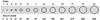 |
Fig. 3 Cursor shapes used to estimate the sizes of the spot umbrae and pores. |
Angle between the direction to the pole of the ecliptic and the zenith as indicated in the drawings and theoretically determined.
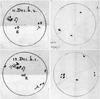 |
Fig. 4 Comparison of the drawings by Scheiner (left) and Harriot (right) on the two days they have common observations. The top row shows the observations of 1611 December 11, at 14 h (left) and at 10 h (right). The bottom row is of 1611 December 13, at 13 h (left) and at 8:30 h (right). The vertical dashed lines in Harriot’s drawings denote the (observed) direction to the zenith, the other dashed lines are the (computed) ecliptic. |
Since neither the printing of the drawings nor the digitization process ensure that the ecliptic is an exactly horizontal line in the image, we also need to add the angle of the printed line, which is obtained by clicking on two points on the line in the image and computing the angle (typically below 1°).
The actual process of measuring the sunspots consists of the following steps: (i) cutting out the solar disk from the full image by clicking on the left-most, right-most, lowest and uppermost limbs of the Sun; this also allows for a certain degree of ellipticity of the solar disk to be measured correctly); (ii) determining the exact angle of the ecliptic line by two clicks, left and right; (iii) setting up the spherical coordinate system as supported by IDL; (iv) clicking on the relevant spots with 13 different cursor sizes (Fig. 3), for which the best fit in position and size to the umbrae and pores are sought visually. In cases where a rotated coordinate system was used to draw spots of crowded regions (see Sect. 2), we can determine the positions if at least one spot was plotted twice, once in the standard ecliptical system, and once in the rotated one. The angle with the disk centre gives us the rotation of the coordinate system for the displaced spots. For 15 spots, this type of duplicate spot was not available, and we omit the positions of these spots, but keep corresponding records in the data file.
Physical areas are then derived from the pixel area of the cursor shapes Acur used for the individual spots, as compared with the total pixel area of the solar disk, Adisk. The heliocentric distance of the spot from the disk centre δ yields the correction for the geometrical foreshortening, and we express the final area in millionths of the solar hemisphere (MSH), i.e. 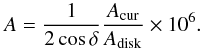 (2)
(2)
4. The observations of 1611–1612
The observations of 1611 October 21 to 1612 April 7 are Scheiner’s first drawings of sunspot observations and are more difficult to measure. The ones of 1611 October 21−December 14 are compiled on a single page in the Rosa Ursina. The page is essentially the same as the one Scheiner sent to the scientific friend Marcus Welser using the pseudonym Apelles latens post tabulam (Apelles hiding behind the scaffold) written on 1611 December 26, and published by Welser in January 1612, together with two earlier letters (Braunmühl 1891). Additional drawings up until 1612 April 7 are available from the letters to Welser of 1612 January 16, April 14, and July 25 (Apelles 1612). We did not have access to the originals, but used the reproductions of the drawings in Reeves & Van Helden (2010) instead.
Some observations show an approximate orientation: the ones of the morning and afternoon of October 22 show the horizon, the ones from 1611 December 10 to 1612 January 11 show the ecliptic; the other drawings have no information about the orientation of the solar disk. The ecliptic was drawn in connection with the expected Venus transit on 11 December which was actually an upper conjuction of Venus and the Sun. The images of 10−13 December also contain the expected path of Venus. The path is confusing as to whether the images may be upside-down or mirrored, since it lies north of the ecliptic, while the true path was south of it. Since the spots are clearly moving from left to right, there was still the possibility that the images are mirrored vertically (a view on a projection screen behind a Galilean telescope). The description reveals, however, that the path was indeed meant to be north of the ecliptic; the accuracy of the ephemeris of Venus was just not good enough (especially of the ecliptic latitude) to place it right at the time (Reeves & Van Helden 2010). For all drawings showing the ecliptic, we computed the angle between the solar axis and the direction to the pole of the ecliptic and set up the coordinate system in the same way as for the observations of 1618−1631. There were 29 observations for which the ecliptic was used in 1611−1612.
There are three options for carrying out the analysis of the remainder of the drawings: (i) using two or more drawings to fix their orientation with the spot displacements owing to the solar rotation (rotational matching); (ii) assuming that all the drawings are plotted in a horizontal system, i.e. the vertical on the book page points to the zenith; or (iii) choosing an arbitrary orientation such that the distribution of spots agrees with today’s expectation of sunspot latitudes.
Method (i) for the rotational matching is the same as described in Arlt et al. (2013). Two or more spots that can be identified in two or more consecutive drawings are used with their measured Cartesian coordinates for a Bayesian inference of their heliographic central-meridian distances and latitudes and the orientation angles of the drawings. A differential rotation, as derived by Balthasar et al. (1986), is used for the solar rotation with a fixed dependence Ω = (14.551−2.87sin2λ)°/day, where λ is the heliographic latitude. The relation was computed from the sunspot group series of 1874−1976 compiled by the Royal Greenwich Observatory.
A Markov chain Monte Carlo search in the parameter space provides us with full posterior probability density distributions for each of the free parameters. In contrast to a best-fit search, they enable us to judge the quality of the rotational matching by the width of the probability density distribution, its skewness, or possible non-uniqueness of probable solutions. The orientations of a total of 23 observations was fixed with the rotational matching.
Since imposing the differential rotation of the Sun to the solution of the orientation does not allow a subsequent determination of the differential rotation in a possible future study, we try to use method (ii) for as many cases as possible. The celestial position of the Sun is provided by the Horizons ephemeris in a J2000.0 system. Since the angle between the solar axis and the direction to the celestial north pole is given in a true-of-date system, we transform the Sun’s coordinates to a system of 1612 using the precess routine from the IDL Astronomy User’s Library. The position of the zenith is computed by the zenpos.pro routine in a true-of-date system as well.
The observations of March and April 1612 are the only ones with a reliable alignment of the zenith direction with the vertical of the images. This was shown by a comparison of measurements with the zenith-assumption and measurements using the rotational matching. Table 4 shows the average deviations of the spot positions between the two methods. While the zenith-assumption delivered fairly consistent results of spot motion across the solar disk, the rotational matching yielded rather broad probability density distributions for the position angles and we kept its results only for 1612 March 17, 19, and April 1. In total, 27 observations were treated with this assumption of a horizontal coordinate system.
Method (iii) was applied only when the first two methods led to improbable spot distributions. We essentially applied a position angle which minimizes the absolute latitudes of the spots. Only four observations were treated with arbitrarily chosen orientations (1611 November 7, 13, 14, and December 8).
The observations of 1611 November 6, 9, 10, 12, and December 24 were omitted entirely because no reasonable match with adjacent observations was possible and the spot distribution appears to be highly improbable. The resulting heliographic latitudes of the spots measured in the 83 observations used from 67 days in 1611−1612 are between −43° and + 42°.
The sizes of the spots were greatly enlarged, and groups of smaller spots were combined into one large spot, as described by Scheiner (see Reeves & Van Helden 2010, for a translation). A size estimate can only be arbitrary at this point, and we chose − to be able to use the 13 cursor shapes − to select the size class that matches roughly half the diameter of the plotted spot. This choice still creates too large areas when converting the disk area fraction of the cursor shape directly to MSH. The areas in the data file are shown with “!” to indicate that these need to be used with care (see Table 6).
Comparison of different coordinate systems adopted for a selected set of observations in 1612.
5. Accuracy of the positions and areas
In the first period of 1611–1612 when Scheiner drew the sunspots with poor quality, there are actually two occasions when Scheiner and Thomas Harriot (1613) observed on the same day (Fig. 4). The images are rotated against each other, since Harriot observed in the morning and Scheiner in the afternoon. There is a fair agreement on the distribution of spots, except that Scheiner noticed a spot near the eastern solar limb on 1611 December 13, which Harriot could not yet detect. Scheiner’s drawings are more detailed, whereas the spots are more exaggerated in size than in Harriot’s drawings. While the drawings look qualitatively similar, we find positional differences of up to 20° on those two days (assuming Harriot’s vertical lines are the direction to the local zenith). This underlines the limited use of the spots in 1611.
Accidentally, Scheiner plotted the positions of one spot in two different image plates (XLVI, spot labelled as “k”, and XLVII, spot labelled as “a”) from 1625 November 6−11. The differences provide us with information on how well the positions may have been reproduced in the plates and are listed in Table 5. The average distance between the positions of the spot in plate XLVI and the corresponding positions in plate XLVII is  . The average “error” of the cursor sizes chosen for the various instances of the spot is 0.5 classes. We kept the positions of plate XLVII, since the spot continued to exist for more days after Nov. 11.
Comparison of the positions of the same spot in two different image plates.
Data format for the positions and areas of individual sunspots observed by Christoph Scheiner and his collaborators.
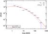 |
Fig. 5 Area distribution of 5555 spots drawn by Christoph Scheiner in 1618−1631, all within a central-meridian distance of | CMD | ≤ 50°. |
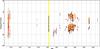 |
Fig. 6 Butterfly diagram of the sunspot positions obtained from the observations by Christoph Scheiner and his colleagues. The ordinate is linear in sinλ. The umbral areas of the individual spots are used to weight the increments accumulating in each time and latitude bin. The approximate activity minimum is the time recently inferred by Neuhäuser & Neuhäuser (2016). |
The areas were taken from pixel counts in the individual cursor shapes and converted into fractions of the solar disk. They are then corrected for foreshortening and given in millionths of the solar hemisphere (MSH). We follow the procedure adopted by Bogdan et al. (1988) to compute the area distribution of the individual umbrae. The result is shown in Fig. 5 and shows a fairly good agreement with their distribution. We interpret the differences from the curve obtained by Bogdan et al. (1988) as follows. Firstly, large spots in particular may be slightly exaggerated in size, an effect seen in many other historic sunspot drawings. At the same time, several of the smallest spots were missed as a result of the observational limits (chromatic telescope). These two effects explain the slight overabundance of spots in large areas and the slight under-abundance of spots between 1.2 and 10 MSH. A correction factor of 0.8 may be suitable for the areas, leading to a perfect match with the curve by Bogdan et al. (1988) in large areas. However, since this is speculation, we have not used any correction factor for the areas in the resulting data file. It would bring the smallest spots to even smaller areas that were very likely not observable.
The smallest spot measurement delivered an area of only 1.2 MSH. A circular spot of this area has an angular extent of 3′′ in the centre of the solar disk. It is doubtful whether the resolving capabilities of Scheiner’s telescopes were as good as that. While King (1955) reported on Galileo’s largest telescope having an aperture of 5.1 cm, but usually being stopped down to 2.6 cm. Abetti (1954) reports on a test of one of the first telescopes of Galileo and found a resolving power no better than 10′′. By the 1620s, the telescopes may have improved, and Scheiner also used a Keplerian setup, which provides better image quality. We found only the following remark about the necessary telescope for the precise enough following of the sunspots’ motion in Scheiner (1630, p. 129-2): The Roman palm measured 74 mm (Brockhaus 1991) leading to impressive suggested lens diameters of 7−15 cm. We did not find an exact aperture of the actual telescopes used, but conclude that the resolution in the 1620s was significantly better than that of Galileo’s early telescopes. Since the drawings − especially the ones of 1624−1631 contain very small spots, we decided to preserve the size information and leave possible recalibrations of the areas to future applications of sunspot data.
6. Data format and butterfly diagram
We use the same table format as the one employed for the spot positions and sizes derived from the observations by Schwabe (Arlt et al. 2013). The format is detailed in Table 6. While the measurements deliver central-meridian distances on the Sun, heliographic longitudes are obtained using the solar disk centre provided by the JPL Horizons ephemeris generator seen from the location in Rome (differences to the various other geographical positions in Europe are extremely tiny).
Since Scheiner drew the sunspots − at first glance − to scale in the years of 1618−1631, we computed physical areas in MSH, corrected for the projection effect towards the solar limb. The observations of 1611−1612 do not show realistic areas. We chose cursor sizes of roughly half the diameter of the spot in the image to compensate for the exaggerated spots to some degree subjectively. Nevertheless, these areas should be used with extreme care.
We define sunspot groups based on Scheiner’s drawings and assigned group numbers. The order of the group numbers has no meaning; for technical reasons they are not ascending monotonically. The groupings were more difficult for 1611, since the groups may have been drawn too large in size. The remaining group definitions were fairly straightforward, since the drawings have a similar look to modern white-light images (except for faculae). The differences to the group definitions made already by Scheiner are not too large. A total of 16 groups were split into two groups, while 10 groups are the result of combining groups together. These numbers increased slightly as compared to Senthamizh Pavai et al. (2016) after another careful inspection.
A total of about 8152 spot positions were derived for 1611−1631. The exact number may still evolve upon further investigations, since the distinction between spots and faculae is not unambiguous (also drawn by dark ink). The resulting butterfly diagram is shown in Fig. 6. A considerable part of a cycle is covered only in the years 1624−1631, where the migration of spot emergences appears to be equatorward. Following Zolotova & Ponyavin (2015), we name this cycle −12. The general migration of sunspot emergence latitude towards the equator is clearly seen. The onset of cycle −12 took place first in the southern hemisphere, while no spot was found in the northern hemisphere. During the second half of cycle −12, the average latitudes of the northern wing are farther away from the equator than in the southern one. The positions are compatible with a time of minimum of fall 1620, as suggested by Neuhäuser & Neuhäuser (2016). Spörer (1889) gives 1619, while Hoyt & Schatten (1998) obtained very low group sunspot numbers for both 1617 and 1618, which are mainly due to an overabundance of zero-detections inferred from generic statements of Simon Marius and Andrea Argoli (incorrectly reported as seen by Riccioli in Hoyt & Schatten1998).
Cycle −13 is more poorly covered. The 1612 observations show the presence of the two butterfly wings nicely, while the 1611 positions are too inaccurate to exhibit the hemispheric division. A slight dominance of the northern hemisphere may be detectable in both 1611 and 1612.
The spot positions and areas are publicly available at the astronomical data centre CDS. Since none of the observational sources before the Maunder minimum covers a sufficient period in time to deliver useful information about a full cycle (the latitudinal distribution of spots in the first place), a unified database of the various data sets is very advantageous.
7. Sunspot group tilt angles
The drawings by Scheiner and his colleagues were then manually inspected for potential bipolar sunspot groups. We restricted the analysis to the very realistic drawings of 1618−1631. The relevant groups were flagged in the positional database and tilt angles were computed according to the method described by Senthamizh Pavai et al. (2015). The data format of the tilt angle data file is exactly the same as in that paper. The total number of tilt angles obtained is 697.
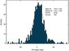 |
Fig. 7 Tilt angle distribution for the observations by Scheiner in 1618−1631. The solid line is a Gaussian fit to the distribution and delivers the full width at half-maximum (FWHM). After Senthamizh Pavai et al. (2016). |
The distribution of the 622 tilt angles within central meridian distances of | CMD | < 60° is shown in Fig. 7. The width of the distribution was derived from a Gaussian fit to the histogram. The average tilt angle of  is slightly lower than values of the 20th century. Values by Wang et al. (2015) for cycles 16−23 range from
  to
to  , if a minimum polarity separation of
  is used to separate unipolar groups with more than one spot from true bipolar groups. Because of the relatively large error margin of the average for Scheiner, we have to conclude that the value is not significantly lower than in the 20th century (see Senthamizh Pavai et al. 2016, for more average tilt angles in the course of four centuries). Most of the data are from 1625−1627, which is roughly the year of solar maximum and two years of the descending activity.
8. Summary
The solar disk drawings with sunspots made by Christoph Scheiner and colleagues in 1611−1631 were digitized and measured. The three sources for the drawings are Scheiner (1630), Scheiner (1651), and Reeves & Van Helden (2010). A total of 8167 spot areas were obtained of which 8152 are accompanied by heliographic positions. All measurements are provided in a database file. The accuracy of both positions and areas are poor for 1611. The positional accuracy improved in the 1612 observations but the spot areas are still highly exaggerated. High quality drawings of 1618−1631 delivered a positional accuracy of about 1°−2° in heliographic coordinates in the solar disk centre, thanks to the large scale of the drawings. The database does not contain spotless days. We refer to the detailed tables by Hoyt & Schatten (1998) for estimates of the spotless days that go beyond what Scheiner (1630) reported.
Sunspot numbers may also be incomplete, as indicated by two groups in Scheiner (1651, Plate I, belonging to p. 7) seen on 1625 May 23−29 and 1626 June 30−July 12, respectively, which were not shown in the images of Scheiner (1630). Since this is the only image with an overlap between the two books, it is not possible to estimate the general completeness.
The positional data support the migration of sunspot emergences towards the equator through cycles −13 and −12. Apart from the very inaccurate 1611 data, there were two groups in 1629 which straddle the equator. On some days, just a few small spots are on the other hemisphere, but on two days (one day for each group), the average polarities sit in opposite hemispheres. Near-equator groups may be interesting for the progress of the activity cycle as recently suggested by Cameron et al. (2013). For the accurate period of 1618−1631, we find that 18 bipolar groups have group centre latitudes of | λ | ≤ 5°.
We computed 697 sunspot group tilt angles from a manually selected set of supposedly bipolar group instances (i.e. the same group may be used on more than one day) for 1618−1631 and provide them in a separate data file. The average tilt angle for these observations is  and is not significantly different from 20th-century values, albeit on the low side. There were 1341 group instances not selected as being bipolar in 1618−1631.
The data are made available at the astronomical data centre CDS5.
Historical archive of sunspot observations at http://haso.unex.es/
Some biographies also give 1575 as the year of birth, e.g. Brockhaus (1992).
Copies of the positional data file and the tilt angle data file are available at http://www.aip.de/Members/rarlt/sunspots
Acknowledgments
We are grateful to Regina v. Berlepsch for digitizing the Rosa Ursina by Christoph Scheiner in the library of Leibniz Institute for Astrophysics Potsdam, to Nadya Zolotova from Sankt Petersburg for drawing our attention to Scheiner (1651), to Ralph Neuhäuser from Jena University for many helpful comments, and to Daniela Luge from Jena University for translating some Latin phrases. V.S.P. thanks the Deutsche Forschungsgemeinschaft for the support in grant Ar 355/10-1.
References
- Abarbanell, C., & Wöhl, H. 1981, Sol. Phys., 70, 197 [NASA ADS] [CrossRef] [Google Scholar]
- Abetti, G. 1954, The History of Astronomy (London: Sidgwick and Jackson) [Google Scholar]
- Apelles, C. S. 1612, De maculis solarib[us] et stellis circa Iovem errantibus, accuratior disquisitio (Augsburg: Ad insigne pinus) [Google Scholar]
- Arlt, R., Leussu, R., Giese, N., Mursula, K., & Usoskin, I. G. 2013, MNRAS, 433, 3165 [NASA ADS] [CrossRef] [Google Scholar]
- Balthasar, H., Vázquez, M., & Wöhl, H. 1986, A&A, 155, 87 [NASA ADS] [Google Scholar]
- Birkenmajer, A. 1967, Vist. Astron., 9, 11 [NASA ADS] [CrossRef] [Google Scholar]
- Bogdan, T. J., Gilman, P. A., Lerche, I., & Howard, R. 1988, ApJ, 327, 451 [NASA ADS] [CrossRef] [Google Scholar]
- Braunmühl, A. 1891, Christoph Scheiner als Mathematiker, Physiker und Astronom (Bamberg: Buchnersche Verlagsbuchhandlung) [Google Scholar]
- Brockhaus. 1991, Brockhaus-Enzyklopädie, 16, Nos-Per (Mannheim: F. A. Brockhaus) [Google Scholar]
- Brockhaus. 1992, Brockhaus-Enzyklopädie, 19, Rut-Sch (Mannheim: F. A. Brockhaus) [Google Scholar]
- Cameron, R. H., Dasi-Espuig, M., Jiang, J., et al. 2013, A&A, 557, A141 [NASA ADS] [CrossRef] [EDP Sciences] [Google Scholar]
- Casas, R., Vaquero, J. M., & Vazquez, M. 2006, Sol. Phys., 234, 379 [Google Scholar]
- Eddy, J. A., Gilman, P. A., & Trotter, D. E. 1976, Sol. Phys., 46, 3 [NASA ADS] [CrossRef] [Google Scholar]
- Eddy, J. A., Gilman, P. A., & Trotter, D. E. 1977, Science, 198, 824 [NASA ADS] [CrossRef] [Google Scholar]
- Harriot, T. 1613, Spots on the Sun, Petworth House, HMC 241 VIII, http://echo.mpiwg-berlin.mpg.de/MPIWG:FAYG83FB [Google Scholar]
- Herr, R. B. 1978, Science, 202, 1079 [NASA ADS] [CrossRef] [Google Scholar]
- Hockey, T., Trimble, V., Williams, T. R., et al. 2007, The Biographical Encyclopedia of Astronomers (New York: Springer) [Google Scholar]
- Hoyt, D. V., & Schatten, K. H. 1998, Sol. Phys., 181, 491 [NASA ADS] [CrossRef] [Google Scholar]
- King, H. C. 1955, The history of the telescope (New York: Dover and London: Griffin) [Google Scholar]
- Landsman, W. B. 1993, in Astronomical Data Analysis Software and Systems II, eds. R. J. Hanisch, R. J. V. Brissenden, & J. Barnes, ASP Conf. Ser., 52, 246 [Google Scholar]
- Malapertius, C. 1620, Oratio habita Duaci dum lectionem mathematicam auspicaretur (Douai: Balthasar Beller) [Google Scholar]
- Malapertius, C. 1633, Austriaca sidera heliocyclia astronomicis hypothesibus illigata (Douai: Balthasar Beller) [Google Scholar]
- Neuhäuser, R., & Neuhäuser, D. L. 2016, Astron. Nachr., 337, 581 [NASA ADS] [CrossRef] [Google Scholar]
- Reeves, E., & Van Helden, A. 2010, On sunspots. Galileo Galilei and Christoph Scheiner (University of Chicago Press) [Google Scholar]
- Rek, R. 2010, Sol. Phys., 261, 337 [NASA ADS] [CrossRef] [Google Scholar]
- Scheiner, C. 1630, Rosa Ursina sive Sol (Bracciano: Andreas Phaeus) [Google Scholar]
- Scheiner, C. 1651, Prodromus pro sole mobili et terra stabili (Nysa, Silesia: Collegium Nissense Societatis Iesu) [Google Scholar]
- Senthamizh Pavai, V., Arlt, R., Dasi-Espuig, M., Krivova, N. A., & Solanki, S. K. 2015, A&A, 584, A73 [NASA ADS] [CrossRef] [EDP Sciences] [Google Scholar]
- Senthamizh Pavai, V., Arlt, R., Diercke, A., Denker, C., & Vaquero, J. M. 2016, Adv. Space Res., in press [Google Scholar]
- Smogulecz, J., & Schönberger, G. 1626, Sol illustratus ac propugnatus (Freiburg im Breisgau: T. Meyer) [Google Scholar]
- Spörer, G. 1889, Ueber die Periodicität der Sonnenflecken seit dem Jahre 1618 (Leipzig: Wilh. Engelmann) [Google Scholar]
- Vaquero, J. M., & Trigo, R. M. 2015, New Astron., 34, 120 [NASA ADS] [CrossRef] [Google Scholar]
- Wang, Y.-M., Colaninno, R. C., Baranyi, T., & Li, J. 2015, ApJ, 798, 50 [NASA ADS] [CrossRef] [Google Scholar]
- Yallop, B. D., Hohenkerk, C., Murdin, L., & Clark, D. H. 1982, QJRAS, 23, 213 [NASA ADS] [Google Scholar]
- Zinner, E. 1957, in Neue deutsche Biographie. Dritter Band, eds. O. Graf zu Stolberg-Wernigerode, et al. (Berlin: Duncker & Humblot) [Google Scholar]
- Zolotova, N. V., & Ponyavin, D. I. 2015, ApJ, 800, 42 [NASA ADS] [CrossRef] [Google Scholar]
All Tables
Numbers of days available for given years as reported by Scheiner (1630), Scheiner (1651), and Reeves & Van Helden (2010).
Angle between the direction to the pole of the ecliptic and the zenith as indicated in the drawings and theoretically determined.
Comparison of different coordinate systems adopted for a selected set of observations in 1612.
Data format for the positions and areas of individual sunspots observed by Christoph Scheiner and his collaborators.
All Figures
|
Fig. 1 Example of an early drawing, indicating the directions and an inner circle annotated as the observed circle. All spots appear twice: once in the inner circle and once in the full circle. |
| In the text | |
|
Fig. 2 Example of a variable ecliptic line to avoid crowdedness. Spots near the eastern and western limbs of the southern-hemisphere groups are rotated above and below their actual position for better visibility. Group a in the northern hemisphere is unaffected. |
| In the text | |
|
Fig. 3 Cursor shapes used to estimate the sizes of the spot umbrae and pores. |
| In the text | |
|
Fig. 4 Comparison of the drawings by Scheiner (left) and Harriot (right) on the two days they have common observations. The top row shows the observations of 1611 December 11, at 14 h (left) and at 10 h (right). The bottom row is of 1611 December 13, at 13 h (left) and at 8:30 h (right). The vertical dashed lines in Harriot’s drawings denote the (observed) direction to the zenith, the other dashed lines are the (computed) ecliptic. |
| In the text | |
|
Fig. 5 Area distribution of 5555 spots drawn by Christoph Scheiner in 1618−1631, all within a central-meridian distance of | CMD | ≤ 50°. |
| In the text | |
|
Fig. 6 Butterfly diagram of the sunspot positions obtained from the observations by Christoph Scheiner and his colleagues. The ordinate is linear in sinλ. The umbral areas of the individual spots are used to weight the increments accumulating in each time and latitude bin. The approximate activity minimum is the time recently inferred by Neuhäuser & Neuhäuser (2016). |
| In the text | |
|
Fig. 7 Tilt angle distribution for the observations by Scheiner in 1618−1631. The solid line is a Gaussian fit to the distribution and delivers the full width at half-maximum (FWHM). After Senthamizh Pavai et al. (2016). |
| In the text | |
Current usage metrics show cumulative count of Article Views (full-text article views including HTML views, PDF and ePub downloads, according to the available data) and Abstracts Views on Vision4Press platform.
Data correspond to usage on the plateform after 2015. The current usage metrics is available 48-96 hours after online publication and is updated daily on week days.
Initial download of the metrics may take a while.