| Issue |
A&A
Volume 595, November 2016
|
|
|---|---|---|
| Article Number | A82 | |
| Number of page(s) | 11 | |
| Section | Catalogs and data | |
| DOI | https://doi.org/10.1051/0004-6361/201628700 | |
| Published online | 03 November 2016 | |
A machine learned classifier for RR Lyrae in the VVV survey
1 Departmento de Estadística, Facultad de Matemáticas, Pontificia Universidad Católica de Chile, Av. Vicuña Mackenna 4860, 7820436 Macul, Santiago, Chile
e-mail: susana@mat.puc.cl
2 Millennium Institute of Astrophysics, 1515 Santiago, Chile
3 Instituto de Astrofísica, Facultad de Física, Pontificia Universidad Católica de Chile, Av. Vicuña Mackenna 4860, 7820436 Macul, Santiago, Chile
4 Gemini Observatory, Chile
5 Unidad de Astronomía, Facultad Cs. Básicas, Universidad de Antofagasta, Avda. U. de Antofagasta 02800, Antofagasta, Chile
6 Departamento de Física, Universidade Federal de Santa Catarina, Trindade 88040-900, Florianópolis, SC, Brazil
7 Departamento de Ciencias Físicas, Universidad Andres Bello, República 220, Santiago, Chile
8 Vatican Observatory, 00120 Vatican City State, Italy
Received: 12 April 2016
Accepted: 25 August 2016
Variable stars of RR Lyrae type are a prime tool with which to obtain distances to old stellar populations in the Milky Way. One of the main aims of the Vista Variables in the Via Lactea (VVV) near-infrared survey is to use them to map the structure of the Galactic Bulge. Owing to the large number of expected sources, this requires an automated mechanism for selecting RR Lyrae, and particularly those of the more easily recognized type ab (i.e., fundamental-mode pulsators), from the 106−107 variables expected in the VVV survey area. In this work we describe a supervised machine-learned classifier constructed for assigning a score to a Ks-band VVV light curve that indicates its likelihood of being ab-type RR Lyrae. We describe the key steps in the construction of the classifier, which were the choice of features, training set, selection of aperture, and family of classifiers. We find that the AdaBoost family of classifiers give consistently the best performance for our problem, and obtain a classifier based on the AdaBoost algorithm that achieves a harmonic mean between false positives and false negatives of ≈7% for typical VVV light-curve sets. This performance is estimated using cross-validation and through the comparison to two independent datasets that were classified by human experts.
Key words: stars: variables: RR Lyrae / methods: data analysis / methods: statistical / techniques: photometric
© ESO, 2016
1. Introduction
Variable stars have historically been a prime tool for determining the content and structure of stellar systems and have had a crucial role in the history of Astronomy. The General Catalog of Variable Stars (Samus et al. 2009) lists over 110 classes and subclasses based on a variety of criteria. The broader distinction that can be made is between variables whose variation is intrinsic or extrinsic, depending on whether the process creating the observed variability is inherent to the star or not, respectively. Arguably the most important group among the intrinsic variables is that of pulsating variables because it contains the classes RR Lyrae and Cepheids, which satisfy a relation between their periods and their absolute luminosities that allows estimating distances, a quantity both fundamental and elusive in Astronomy. For a current review of the physics and phenomenology of pulsating stars, we refer to the recent monograph by Catelan & Smith (2015).
RR Lyrae stars are of special importance for the purposes of exploring the distances and properties of old stellar populations. They have periods in the range ≈0.2–1 day and are found only in populations that contain an old stellar component with an age ≳10 Gyr. Based on their light-curve shapes, RR Lyrae were originally separated into subclasses a, b, and c, also known as their Bayley type (Bailey 1902). It was later recognized that classes a and b pulsate in the fundamental radial mode, whereas subclass c does so in the first-overtone radial mode (Schwarzschild 1940), and therefore modern usage distinguishes only between RR Lyrae types ab and c (sometimes alternatively termed RR0 and RR1, respectively), and additional (but much less frequent) subclasses have been introduced for other pulsational modes.
Arguably the most important property of RR Lyrae is that they can be used as standard candles, and they have played a prominent role in determining the three-dimensional structure of our Galaxy ever since Shapley used them to determine the distance of various globular clusters and used that fact to determine the distance to the Galactic center (Shapley 1918). An obvious use of RR Lyrae would then be to map the structure of the Galactic bulge, but that is an observationally challenging task because of the high extinction present and the large area to be covered. Providing such a three-dimensional mapping of the bulge using RR Lyrae was one of the main motivations for the Vista Variables in the Via Lactea (VVV) ESO Public Survey (Minniti et al. 2010), which covered ≈520 deg2 of the Galactic bulge and disk with the VISTA telescope in Paranal. The VVV will catalog ≈109 sources in the ZYJHKs bandpasses, with a variability of the bulge probed with ~100 epochs in Ks over a total time span of >5 yr.
With an expected yield of 106−107 variable stars over its whole footprint, human classification is not a viable path to identify the different variability classes that will arise from the VVV. Machine-learned procedures that classify variable stars, called the “classifier”, become a must in view of these numbers and will become even more so as the size of future synoptic surveys such as the Large Scale Synoptic Telescope (LSST, Ivezic et al. 2008) become operational. The classifier receives as a minimum input a time series of measured luminosity at irregularly sampled times, and outputs a score of confidence of membership in a specific class.
The aim of this study is to build an automated procedure to classify RR Lyrae type ab (from now on RRab) stars from the VVV survey. The performance of automated classifiers of variable sources in the optical has been assessed in several previous studies (e.g., Debosscher et al. 2007; Dubath et al. 2011; Richards et al. 2011; Paegert et al. 2014; Kim & Bailer-Jones 2016), which followed a similar approach. First we need to assess whether the variable is periodic, and if so, the period of the time series needs to be estimated. This is a crucial and challenging step because the astronomical time-series are measured irregularly over time, often with intervals of high and low cadence. A parametric model is then fit to the folded light-curves. From the parameters of the model and directly from the light curves, a set of characteristics or features are then extracted. The final step is to decide on a specific function of the features that estimates the membership scores, and this is done for supervised classifiers such as those mentioned by using a training set of light curves that have been labeled by a human expert.
The near-infrared (NIR) offers at least two challenges as compared to the optical. First, it is intrinsically harder to classify RRab in the infrared because their amplitudes are smaller than in the optical, making them harder to detect at a given signal-to-noise ratio level, and the light curves are more sinusoidal, which increases the risk of confusing them with other types of variables, particularly close binaries. Second, as opposed to the visible, in which there are many high-quality light curves with which supervised classifiers can be trained, in the NIR high-quality templates are scarce. This situation is now changing thanks to efforts such as the VVV Templates project (Angeloni et al. 2014).
The structure of this paper is as follows. In Sect. 2 we describe the data, in Sect. 3 we describe the method for feature extraction together with the classification algorithm and its formal performance, and in Sect. 4 we further illustrate its performance by comparing the results with those achieved by a human expert classifier on various datasets extracted from the VVV. We close in Sect. 5 with a summary and our conclusions.
2. Data
2.1. VVV ESO public survey
The Vista Variables in the Via Lactea (VVV) is an ESO public survey that is performing a variability survey of the Galactic bulge and part of the inner disk using ESO’s Visible and Infrared Survey Telescope for Astronomy (VISTA). The survey covers 520 deg2 in the ZYJHKS filters for a total observing time of ≈1900 h, including ≈109 point sources and an estimated ~106−107 variable stars. The final products will be a deep NIR atlas in five passbands. One of the main goals is to gain insight into the inner Milky Way origin, structure, and evolution. This will be achieved, for instance, by obtaining a precise three-dimensional map of the Galactic bulge. To achieve this goal, RR Lyrae stars are of particular importance. There are many RR Lyrae in the direction of the bulge and, because they are very old, they are fossil records of the formation history of the Milky Way. For a detailed account of the VVV see Minniti et al. (2010), and for a recent status updated with emphasis on variability see Catelan et al. (2014).
2.2. Light-curve extraction and pre-processing
Aperture photometry of VVV sources is performed on single-detector frame stacks provided by the VISTA Data Flow System (Irwin et al. 2004) of the Cambridge Astronomy Survey Unit (CASU). A series of flux-corrected circular apertures are used as detailed in previous publications (Catelan et al. 2013; Dékány et al. 2015). We denote the apertures as { 1,2,3,4,5 } , and they are extracted in aperture radii of  arcsec.
When the Ks-band light curves are extracted, stars with putative light variations were selected using Stetson’s J index (Stetson 1996,Eq. (1)), taking advantage of the correlated sampling of the Ks data, that is, the fact that the light curves are sampled in batches of 2–6 points measured almost at the same instance. We estimated significance levels of this statistic as a function of the number of points by Monte Carlo simulations using Gaussian noise, and selected objects showing correlated light variations above the 99.9% confidence level.
After selecting the curves that showed evidence of variability, we proceeded to eliminate individual observations that have anomalously large error bar estimates, as these indicate epochs with anomalous observing conditions that provide little information. If  is the set of uncertainty estimates for a light curve with n points, then we eliminate any points whose σi values are >5σ from the distribution mean, where σ ≡ Var({σi}).
2.3. Training sets
To use a supervised classification scheme, we need a training set that is used by the classifier to learn how RR Lyrae are characterized in feature space. In this paper, we decided to restrict ourselves to the ab-type RR Lyrae stars, as RRc stars have smaller amplitudes (hence noisier light curves) and are frequently very difficult to distinguish from contact eclipsing binaries. The training sets were known instances of the RRab class, ideally observed with a cadence and precision similar to that of the target data that arises from the VVV. To retrieve a training set from the VVV itself, we used light curves consistent with being variable from the bulge fields B293, B294, and B295, located around Baade’s window. These fields are well covered by OGLE-III (Szymański et al. 2011), and given that the OGLE-III I-band catalog is deeper than what we achieve with VVV in this region of the bulge, we assumed that all RRab in the three chosen fields that can be detected with VVV are present in the OGLE-III catalog. Therefore, we assembled a training set for each of the bulge fields by cross-matching the RRab catalogued in OGLE-III with the light curves extracted from VVV data.
In addition to the training set above, we used Ks IR light curves gathered as part of the VVV Templates project (Angeloni et al. 2014). This project is a large observational effort aimed at creating the first comprehensive database on stellar variability in the NIR, producing well-defined high-quality NIR light curves for variable stars belonging to different variability classes, such as RR Lyrae, Cepheids, and eclipsing binaries. The main goal of the project is to serve as a training set for the automated classification of VVV light-curves.
Table 1 shows the numbers of RRab light curves versus those belonging to other classes in each of the training datasets considered in this study. We note that in principle we have color information for our objects, but similarly to other studies (e.g., Kim & Bailer-Jones 2016), we have decided not to use that information to train the classifier. The reason is that the footprint of the VVV is subject to a very wide range of extinction values (e.g., Gonzalez et al. 2012), and thus usage of color information would imply the need to account for the reddening, which would introduce another level of complexity.
Number of RRab versus other classes in the training datasets.
2.4. Measuring classifier performance
To assess the performance of the classifiers, we estimated four measures of quality using tenfold cross validation: precision, recall, F1, and AUC (defined below). In tenfold cross-validation, the classifier is trained with nine tenths of the training set, and the performance of the classifier is assessed with the remaining tenth. This is repeated ten times, and each time, a different tenth of the training set is held out, obtaining ten estimates of performance that are then averaged.
-
Precision is the probability that a randomly selected objectpredicted to be in a target class does belong to the target class. Wedenote precision by P. We note that the false-discovery rate, that is, the rate of false positives, is 1−P.
-
Recall is the probability that a randomly selected objected belonging to a target class is indeed predicted to be in that class. We denote recall as R.
-
F1 measure, defined as the harmonic mean between P and R, that is,
 . As a weighted average of precision and recall,
it is a measure of the accuracy of the classifier, where a perfect accuracy would
imply values close to one.
. As a weighted average of precision and recall,
it is a measure of the accuracy of the classifier, where a perfect accuracy would
imply values close to one. -
Area under the curve (AUC) is the area under the so-called receiver operating characteristic (ROC) curve, which shows the true-positive rate as a function of the false-positive rate. Values close to 1, which is the maximum possible, are best because they indicate a classifier that quickly achieves a high true-positive rate with a correspondingly low false-positive rate.
In addition to testing the performance using cross-validation, we used distinct datasets extracted from the VVV that were not used at all in the training and in which a catalog of RRab had been built by a human expert. We used two such datasets: (1) a catalog of RRab in the Galactic globular clusters 2MASS-GC 02 and Terzan 10 (Alonso-García et al. 2015). These RRab were classified based on their light-curve shape and their position in the HR diagram. (2) A catalog of RRab in the outer bulge area of the VVV (Gran et al. 2016, the outer bulge refers to VVV fields with b< −8 deg). This is an extension of previous work reporting the RRab content of one single tile of the VVV (Gran et al. 2015). The RRab in this work were classified solely based on their shape by a human expert.
3. Methods
3.1. Period estimation
We estimated the periods of the light curves using the generalized Lomb-Scargle periodogram (GLS Zechmeister & Kürster 2009). We restricted the periodogram to frequencies satisfying f1< 5 day-1. We also eliminated all light curves whose highest Lomb-Scargle peak had a value ≤0.3. The threshold was determined using the Lomb-Scargle peaks of known RRab in our VVV training fields; no source has a Lomb-Scargle peak with a value lower that the chosen threshold. Finally, we eliminated all curves with ≤50 observations (VVV observations are clustered, usually in groups of ≈4, so that the chosen cut corresponds to cutting light curves with typically ≲15 epochs).
3.2. Harmonic model light-curve fit
After we determined the first frequency, we fit a harmonic model to the light curves. Here y(t) is the observed light intensity at time t from a given variable star, ŷ(t) = a + bt is the linear trend estimated from a linear regression model of the photometric time series, and r(t) = y(t)−ŷ(t) is the photometric time series with the linear trend subtracted. Then we iterated between two steps as described below.
-
1.
We performed a Fourier analysis of r(t) to determine additional periodicities that might exist using GLS. The periodogram was calculated and the highest peak was selected. The corresponding frequency f was used to find the parameters of the following harmonic fit using the method of weighted least-squares estimation using the inverse measurement variances
 as weights:
 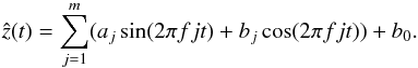 (1)When this model was fit using the first frequency f1, an outlier rejection was performed (see below). This was not done for subsequent frequencies.
 -
2.
We reassigned r(t) through r(t) ← r(t)−ẑ(t).
In words, we first subtracted the linear trend from the photometric time series. Then, using the periodogram, we identified the largest peak and use the corresponding frequency to fit a harmonic model with m components. This new curve, together with the linear trend, was subtracted from the photometric time series and a new frequency was searched for in the residuals using the periodogram. The new frequency was used to fit a new harmonic model. This process continued until n frequencies were found and n harmonic models with m components were estimated.
Finally, the n frequencies were used to make an harmonic best fit to the original light curve through weighted least squares of the full model given by 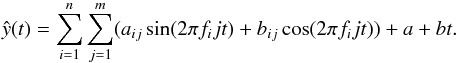 (2)Following Debosscher et al. (2007), we used n = 3 frequencies and m = 4 harmonics to characterize the light curves.
3.3. Rejection of outliers and poor light curves
After finding the first frequency f1 and fitting an harmonic model with f1 only, we rejected outliers from each light curve. We obtained a smooth estimate of the phased light curve using smoothing splines obtained from the R function smooth.spline, with the parameter that controls the smoothing set tospar=0.8 (this value was chosen based on a best-fit measure of folded light curves). Then, we performed an iterative σ-clipping procedure to the residuals around the smooth model of the phased light curve. Assuming Gaussian errors, we removed outliers at the 4σ level or above and estimated the dispersion of the residuals reliably by setting σ = 1.4826 × MAD, where MAD is the median absolute deviation.
We also eliminated from our sample light curves with either too low signal-to-noise ratios or patchy phase coverage. In detail, we eliminated all light curves whose scatter around the phased light curve was not significantly different from the raw light curve by eliminating all curves whose median absolute deviation about the phased light curve was >0.8 times the median absolute deviation of the raw light curve, or in other words, light curves whose scatter was not significantly reduced after folding with the period (this corresponds in terms of the feature p2p_scatter_pfold_over_mad to 1/p2p_scatter_pfold_over_mad >0.8). To eliminate curves with incomplete phase coverage, we eliminated all curves where 1−Δφmax< 0.8, where Δφmax is the maximum of the consecutive phase differences  , where N is the number of measurements, and we took φN + 1−φN ≡ 1 + φ1−φN.
3.4. Feature extraction
Features were extracted from the raw and phase-folded light curves, and from the parameters of the best-fitting harmonic model. We adopted most of the features proposed in Debosscher et al. (2007), Richards et al. (2011) and Richards et al. (2012b), and we introduced a few new features specifically designed to better distinguish RRab from close binaries such as those of the W UMa type, which were our most troublesome contaminant. Table 2 lists all the features used by our classifier, along with a short description and a reference to the literature when adopted from previous work. A total of 68 features were extracted to be used by the classifiers.
List of light-curve features.
An important set of features was derived from the harmonic fit, but care must be taken to choose parameter expressions that are invariant to time translations. The frequencies fi, together with the Fourier parameters aij and bij, constitute the direct set of parameters with which we modeled the light curves. A drawback of this representation is that the parameters are not invariant to time translation. In other words, when two light curves from the same star are observed that do not coincide in its starting time, then these two light curves will have two different sets of parameters to represent the same star. To obtain parameters that uniquely represent a light curve, we transformed the Fourier coefficients into a set of amplitudes Aij and phases  as follows:
![\begin{eqnarray} &&A_{ij}=\sqrt{a_{ij}^2+b_{ij}^2}, \\[3mm] &&\phi_{ij}^{'}=\arctan(\sin(\phi_{ij}),\cos(\phi_{ij})), \end{eqnarray}](/articles/aa/full_html/2016/11/aa28700-16/aa28700-16-eq114.png)
where 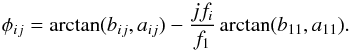 (5)We note that φ11 was chosen as the reference and was set to zero and that
  takes values in the interval [−π,π].
We used two additional features in this work, which are listed at the end of Table 2. As mentioned in Sect. 1, the RRab light curves in the IR are of lower amplitude and more symmetrical than in the optical. This makes confusion with close binaries that have periods in the range of RRab a very challenging contaminant for the classifier to distinguish. Even if subtler in the NIR, one of the features that often distinguishes RRab is some level of asymmetry around the peak of the light curve, with a steeper ascent and a slower descent. As we show below, even though one of the features we introduced has some importance, it is not a very large one. This is not surprising once it is realized that some bona fide RRab are extremely symmetrical in the IR. We show in Fig. 1 the VVV (Ks) and OGLE (IC) light curves of a known RRab classified by OGLE. The figure clearly shows the challenges of classifying RRab in the IR as compared to the optical. It is also clear from the figure that any feature that tries to quantify asymmetry in the peak cannot be very relevant for a curve such as this one, and the classifiers learn this fact.
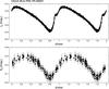 |
Fig. 1 Example of a known RRab classified by OGLE using an optical IC light curve (upper panel). It shows a very symmetric light curve in the infrared (lower panel, Ks light curve from the VVV). |
3.5. Choice of classifier
To choose the best classifier for RRab, we tested several well-established classifiers. We refer to Hastie et al. (2009) for a detailed description of many of the algorithms below (see also Ivezić et al. 2013); more detailed documentation can be found in the documentation of the functions we use. The classifiers were implemented using functions in the R language (R Core Team 2015); we indicate the functions as well as the options or parameters when appropriate.
-
Logistic regression classifier. We used the glm function of thestats library to perform the regression.
Classification tree (CART). We used the rpart function of the library with the same name.
Random forest (RF). We use the randomForest function of the randomForest library in R with parameter ntree=500 (number of trees) and mtry = 20 ( number of variables at each tree). To set these parameter values, we assessed the performance of the classifier on a grid of values. ntree took values in the interval [100–1000], and mtry took values in the interval [1, p], where p is the number of features. Our final classifier includes only 12 out of the 68 original features; for the final classifier the parameter mtry was set to 3.
Stochastic boosting (SBoost) is implemented with the ada function of the ada library in R. Two versions of this classifier were tested. The first has parameters loss = “exponential” and parameter type = “discrete” (denoted as Sboost1), and the second has parameters loss = “logistic” and parameter type = “real” (denoted as Sboost2), both with parameter max.iter = 500. All combinations of loss functions with the different options for the type parameter were evaluated, and the max.iter parameter was assessed in the interval [100, 1000]. Based on performance, we chose to consider SBoost1 only in what follows, and we write SBoost for short.
AdaBoost (ADA, short for adaptive boosting) is implemented with the boosting function of the adabag library in R. Ada.M1 uses the AdaBoost.M1 algorithm (Freund et al. 1996) with the Breiman weight-updating coefficient (option coeflearn = “Breiman”), while Ada.SAMME uses the AdaBoost SAMME (Zhu et al. 2009) algorithm with the option coeflearn = “Zhu”. The coeflearn values represent different options for weighting the “weak” classifiers based on the misclassification rate. In both classifiers we assessed the number of trees (parameter mfinal) in the interval [100, 1000], and based on cross-validation, chose ntrees = 500. Both algorithms have the parameter boos set to TRUE, and therefore, a bootstrap sample of the training set was drawn using the weights for each observation on that iteration. Based on performance, we chose to consider Ada.M1 only in what follows.
A support vector machine (SVM) classifier with a polynomial kernel is implemented with the function svm of the e1071 library with parameters degree=2 and nu=0.1. The choice of radial basis, lineal, polynomial, and sigmoid kernels were assessed, and we found that the best performing was the polynomial kernel.
LASSO is a penalized likelihood classifier that implements L1 penalization. Implementation was made with the glmnet function of the glmnet library with options family = “Binomial” and nlambda = 1000. The latter was chosen after testing performance in the range [100, 10 000]. The parameter α, the elasticnet mixing parameter, was tested in the range [0, 1] and set to 1 (giving thus a LASSO, α = 0 corresponds to ridge regression).
Multiple hidden neural networks (MHNN) implemented with the nn.train function in the deepnet package in R, and parameters hidden = 10, activationfun = “sigm” (a sigmoid activation function), batchsize = 1500 and numepochs = 2000. The parameters were set after the classifier performance was assessed, testing the parameters batchsize in the interval [100, 2000] and the number of hidden layers in [1, 20].
Deep neural network (DeepNN) implemented with the dnn function in the deepnn package in R. A sigmoid activation function and five hidden layer were used, with parameter batchsize = 1500, numepochs = 2000, and ten hidden layers. The classifier performance was assessed, testing the parameters batchsize in the interval [100, 2000] and the number of hidden layers in [1, 20].
Cross-validation performance of classifiers on the templates+B293+B294+B295 training set, using all features.
3.6. Choice of aperture for photometry
After we selected the best classifier, we assessed whether the selection of an aperture from which we estimated the features of the light curves affected the classification performance. We implemented three strategies to select the aperture. The first was to fix the aperture size to be equal for all variable stars. We call this strategy fixAper(i) for aperture size i (this gives us five strategies). Second, we chose for each light curve the aperture size that achieved the minimum sum of squared measurement errors and called this strategy minError. Third, similarly to Richards et al. (2012a), we developed a kernel density classifier that outputs probability scores for each aperture based on the median of the mean magnitudes at the five apertures.
The kernel density for aperture 1, for instance, g1, was estimated using the mean magnitudes of all the light curves whose minimal sum of squared measurement errors was achieved at aperture 1. In a similar way, we estimated the kernel densities for the remaining four apertures, g2,g3,g4,andg5. Figure 2 shows the densities for each aperture size. We also estimated the proportion of light curves that achieved the minimum sum of squared measurement errors at each aperture, for example, π1,π2,π3,π4,andπ5, estimates of which are shown in Fig. 3. Unlike Richards et al. (2012a), we developed a soft thresholding classifier to choose an optimal aperture. For a new light curve, we chose the aperture whose probability p(j | y) was the highest, where 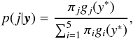 and y∗ is the median of the mean magnitudes at all five apertures. The classifier selects the aperture with the highest score. We call this third strategy KDC.
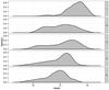 |
Fig. 2 Kernel density estimates of the mean magnitude of curves with the minimum sum of squared errors at each aperture size. |
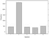 |
Fig. 3 Number of light curves with the minimum sum of squared errors at each aperture size. |
For each variable star, we selected the time series based on a particular strategy for selecting aperture and followed the full procedure of extracting the features and training the classifiers. We evaluated the performance of the seven strategies using the Ada.M1 classifier, which we previously determined to be among the top performers. Results are shown in Table 4. We used cross-validation on variable stars from the B295 field to estimate the performance of the Ada.M1 classifier under different strategies. Table 4 shows that the strategies KDC and fixAper(2) are the best performers. Given that most sources have the minimum sum of squared errors for aperture i = 2, it is natural that KDC is equivalent in terms of performance to fixAper(i), but for source magnitude distributions where this is not the case, we would expect KDC to be better. We note that KDC outperforms minError, a strategy often used to choose an aperture.
F1 Measure by aperture choice strategy for Ada.M1.
3.7. Feature selection
In Sect. 3.5 we used all 68 features to assess the best classifier. It is clear that not all features have the same effect on the classification, and we can measure how important each one of them is for the classification. In Fig. 4 we show the features ordered by importance, with the most important at the top. The relative importance of the predictor variables was computed using the gain of the Gini index given by a variable in a tree and the weight of the tree. As expected, by far the most important feature is the fundamental frequency (f1). As stated in the Introduction, RRab have periods in a very well-defined range, and it is therefore natural that these characteristics are the most prominent in deciding whether a curve belongs to the RRab class. It also underscores how important it is to estimate the period correctly, and there have been many efforts in assessing the best tools for period finding in astronomical time series (e.g., Graham et al. 2013). Therefore, obtaining accurate and reliable periods is crucial for our classification scheme: if the period is inaccurate, the classification is bound to be imprecise. The next features in importance are all based on the harmonic fit to the data, and the first unrelated to this is p2p_scatter_2praw.
Based in Fig. 4, we determined that using 12 features suffices to obtain the final best performance. While in principle we could have kept all 68 features, doing so introduces a larger scope for noise being introduced by features that are not very informative and that particularly for faint sources can be noisy. The choice of 12 features was made on the basis that by the twelfth feature, A12, the F1 measure (x-axis in the figure) has reached maximum, and adding the next feature even slightly decreases the performance. This means that we have reached at the twelfth feature the best performance over the level around which additional features do not add significant information.
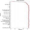 |
Fig. 4 Feature importance using the Ada.M1 classifier. Based on this graph, we chose to consider only the 12 most important features in the final classifier. |
Cross-validation performance of classifiers on the templates+B293+B294+B295 training set, using the best 12 features.
The cross-validation estimates of performance that results after training all of the classifiers using only the 12 more important features are summarized in Table 5. It is interesting to note that the performance of the AdaBoost and SBoost classifiers is very similar to that for all features. This is a desirable property as the performance is not overly sensitive to the particular choice of features. On the other hand, other classifiers change their performance significantly. Of particular interest is the fact that the performance of the widely used random forest classifiers is more similar to that of of AdaBoost and SBoost, although it is still lower.
3.8. Sensitivity to training set choice
An important step in building a classifier is to select an appropriate training set that captures the variability of the data because when the training set is not representative, the resulting classifier is bound to fail for some types of objects. To test our sensitivity to the training set choice, we trained our classifier using different training sets by taking different subsets out of the four available sets (templates, B293, B294, and B295, see Sect. 2.3). In Table 6 we show the results of this exercise using the Adaboost.M1 classifier, showing the F1 measure for different combinations of training and test sets; we note that in this case we measured the performance with a test set that was disjoint from the training. The first row shows the performance for the classifier trained only on templates (T), the following three rows shows the performance for the classifier trained using templates plus B295, B294, or B293 respectively. The next three rows are similar to the previous three, but now two complete fields are incorporated into the training set. The last two rows show the performance of the classifier with all of the curves from templates plus 90% (80%) of the curves from the three fields. As evident from Table 6, the performance is best when we include curves from templates and all three fields. It does not vary significantly between having 80% or 90% of the curves over the expected random variations in the F1 performance, which for Adaboost.M1 was expected to be on the order 1%. We conclude that our choice of training set of templates+ 80% B293 + 80% B294 + 80% B295 does not bias our results in a significant way, as assessed by training the classifier.
F-measure by training set (Adaboost.M1).
3.9. Final classifier
Building upon our extensive experiments, as described above, we defined our final classifier in the following way. We used templates+ 80% B293 + 80% B294 + 80% B295 as our training set, selected the aperture of each curve based on KDC, and adopted an Ada.M1 classifier using the following 12 features of the 68 listed in Table 2 (ordered by importance):
-
1.
f 1
-
2.
φ 12
-
3.
φ 13
-
4.
A 11
-
5.
p2p_scatter_2praw
-
6.
P 1
-
7.
R1
-
8.
skew
-
9.
A 12
-
10.
A 13
-
11.
φ 14
-
12.
p2p_scatter_pfold_over_mad.
The F1 measure as estimated from cross-validation is ≈0.93. We refer to this classifier in what follows as the final or optimal classifier. It is interesting to compare this performance with that obtained by similar methods in the optical for ground-based studies. The machine-learned classifier implemented for ASAS by Richards et al. (2012a) attains an F1 performance of ≈0.96 for RRab classification (see their Fig. 5), or about a factor of ≲2 better that what we achieve in terms of the expected number of false positives or negatives. The increased performance in the optical is expected given the larger amplitudes and more asymmetric shape in those bands, and the optical should therefore be taken as an upper bound of what supervised classification could achieve for the VVV data. Of course the data are not necessarily directly comparable, and the ASAS data used by Richards et al. (2012a) have a larger number of epochs (mean of 541, whereas the VVV has typically on the order of 100). We conclude from this comparison that our finally chosen performance is fairly close to what we can think of as an upper bound for supervised classification methods for RRab.
4. Performance on independent datasets
In the sections above, we measured the performance of various classifiers, including what we chose as the optimal classifier. In this section we compare the performance of our classifier with the gold standard human expertise on two datasets mentioned in Sect. 2.4: (1) a catalog of RRab in the Galactic globular clusters 2MASS-GC 02 and Terzan 10 (Alonso-García et al. 2015); and (2) a catalog of RRab in the outer bulge area of the VVV. This comparison is particularly relevant as it allows us to assess the generalization performance of the classifier on different datasets in which flux measurements do not necessarily follow the same conditions in cadence, depth, etc. as our training set. The cross-validation evaluation of the performance of our optimal classifier gives an F1 measure of ≈93% using a score threshold of 0.548, so that if this performance generalizes well, we would expect the harmonic mean of the number of false positives and false negatives to be on the order of 7%.
4.1. RRab in 2MASS-GC 02 and Terzan 10
Alonso-García et al. (2015) classified 39 variables as RRab. In addition to the light curves, Alonso-García et al. (2015) used color information to assess the nature of the variables, and optical light curves from OGLE when available. Therefore, there is high confidence on the nature of the stars classified as RRab. We note that this comparison is biased against our machine-learned classifier, which only had the VVV light curves as input for the classification. The distribution of scores for the RRab classified by Alonso-García et al. (2015) (true positives), and the false positives and negatives, are shown in Fig. 5. As evident in the figure, the great majority of known RRab are classified correctly as such by the classifier. Six sources, or ≈15% of the sample, are false negatives. The periods for these sources are consistent with those of RRab, and because they are not symmetrical, they were classified as RRab by Alonso-García et al. (2015).
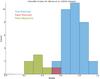 |
Fig. 5 Histogram of scores obtained by the classifier for the light curves of the sample presented by Alonso-García et al. (2015). Shown are the true positives (sources classified by Alonso-García et al. 2015, as RRab), false positives, and false negatives. |
On the other hand, there were formally two false positives, or ≈5% of the sample at face value, which are shown in Fig. 6. We discuss each in turn. Terzan10_V113, shown in panel (a), was classified as an eclipsing binary in Alonso-García et al. (2015) because of its very symmetric nature. It is not classified as an RRab by OGLE either, reinforcing its status as a non-RRab. In light of the very symmetric nature of some RRab in the IR (cf. Fig. 1), it is not surprising that variables with the correct periods and amplitudes for RRab are classified as such even if they are very symmetric. One additional variable was classified as RRab, but was not present as a variable in the Alonso-García et al. (2015) catalog. Its internal IDs is 21089, and it is shown in panel (b) of Fig. 6. Variable 273508 is an RRab detected by OGLE (OGLE_BLG_RRLYR-33508) that was inadvertently left out in Alonso-García et al. (2015). It is most likely a field RRab because it is beyond the tidal radius of Terzan 10, and it is also too bright to be part of the cluster. In summary, after studying the formal false positives in detail, we conclude that one is most likely a RRab and that the classifier therefore has only one false positive.
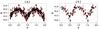 |
Fig. 6 Two sources that were nominally false positives: a) Terzan10_V113; b) internal identifier 273508. One of them a) is a bona fide false positive, while the other b) is a true positive that was not flagged as such in the work of Alonso-García et al. (2015) (see text). |
All in all, the harmonic mean of false positives and false negatives is 1.71 or ≈4.4%, consistent with the cross-validation estimate and even better than expected.
4.2. RRab in the outer bulge area of the VVV
Gran et al. (2016) analyzed 7869 light curves consistent with being variable in the outer bulge region of the VVV survey and performed a human classification into RRab or “other”. The classifier presented in this work was run on the same dataset, and its results contrasted with the human expert performance. There were 1019 light curves classified as RRab in Gran et al., of which 939 passed the cleaning process detailed in Sect. 3.3. All the sources that were formally false positives and false negatives in comparison with Gran et al. (2016) were reassessed by eye; this was necessary because our processing of the light curves was different and in particular the periods were estimated in a different fashion, leading in some cases to bona fide RRab in our dataset that were not catalogued in Gran et al. We found that among the 939 sources there were 50 false negatives, and the classifier gave an additional 177 false positives, which is a total of 1066 sources that were deemed RRab by the classifier. The distributions of scores for the outer bulge light curves is shown in Fig. 7. The harmonic mean of the number of false positives and negatives is ≈78, or ≈8% of the sample size, slightly lower but fully consistent with the F1 measure as estimated from cross-validation on the training set.
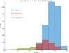 |
Fig. 7 Histogram of scores obtained by the classifier for the outer bulge light-curves of the sample used by Gran et al. (2016). Shown are the true positives (sources classified by as RRab), false positives, and false negatives. |
We conclude that independent datasets that were not used in the training fully confirm the performance estimates obtained using cross-validation of the training sets.
5. Summary and conclusions
We have presented the construction of a machine-learned RR Lyrae type ab classifier for the NIR light curves arising from the VVV survey. After preprocessing light curves based on the number of observations and outliers based on standard errors, we searched for an appropriate training set and the best aperture for each light-curve to feed the classifier. We looked for the best supervised classifier among a wide variety of algorithms and found AdaBoost classifiers to consistently achieve the best performance. It is interesting to note that an AdaBoost classifier performed slightly better than random forests, which have been gaining much popularity for classification problems in Astronomy, and in particular, they have seen wide use recently in the problem of variable star classification (e.g., Dubath et al. 2011; Richards et al. 2012a; Armstrong et al. 2016). Similar to random forest, the AdaBoost classifier is an ensemble method. These types of methods combine scores from several “weak” classifiers to obtain better predictive performance. The key attribute of the AdaBoost is that it is adaptive in such a way that samples that have been incorrectly classified by the previous “weak” classifiers are attributed higher weights in subsequent classifiers. Thus, the classifier adaptively concentrates on the training instances that are more difficult to classify. In addition to being a slightly better performer, the AdaBoost classifier performance was stable with respect to sign all features or a restricted set of the most important features. This stability is welcome because it results in a more forgiving behavior with respect to the set of features chosen for a final classifier as long as there are enough features to capture the bulk of the classification problem. We therefore recommend that AdaBoost always be tried as an alternative, in particular for the problem of variable star classification.
We extracted 68 features for each light curve and found that 12 were enough to achieve the best performance. The most important feature is the period, as expected because of the very well-defined period range of RRab variables. Various phases and amplitudes of a harmonic fit to the light curve are also important in defining the RRab class. The performance of the chosen classifier, the AdaBoost.M1 algorithm (Freund et al. 1996), with the 12 most important features reaches an F1 measure of ≈0.93. This performance was estimated using cross-validation on the training sets, and was verified on two completely independent sets that were classified by human experts.
The performance achieved by the classifier constructed in this work will allow us to address one of the main aims of the VVV survey: the identification of RRab over the full survey area with an automated, reproducible, and quantitative classification tool. The expected harmonic mean between false positives and false negatives is ≈7% when using a score threshold of 0.548, which maximizes this measure. When purer or more complete samples are needed for particular science aims, the threshold on the classifier score can be adjusted as the needs dictate. For example, if a very complete and pure sample is desired, a lower score threshold might be used than the one that maximizes the F1 score, and then the list might be culled even further using ancillary information. The benefit of the classifier in this case is to reduce the number of candidate sources in an efficient, homogenous, and reproducible way.
Ancillary data to further assess the nature of variable light curves could come from the VVV itself, as there is also color information that is not being used by the classifier. The latter fact is by design, to avoid the complications and potential spatial biases that could be introduced in a classification scheme that uses colors. Because analyzing the spatial structure of the Milky Way bulge is one of the main aims of the VVV, we desire the classification procedure to be as free of spatial biases as possible. Of course, reddening will introduce spatial variations in the depth of the sample, but the classification should perform similarly for light curves of similar signal-to-noise ratio and phase sampling.
There are many more variables of interest in the VVV in addition to RRab (see, e.g., Catelan et al. 2013). Future work will address the construction of machine-learned classifiers for them. We aim to design custom binary classifiers for sources of interest, such as done in this work, but also a single multi-class classifier similar to that of Richards et al. (2012a). We also plan to explore alternative classifier schemes beyond the supervised classification scheme employed here; an interesting possibility is to explore the use of Kohonen self-organizing maps, which has been tried before for the problem of classifying light curves (Brett et al. 2004; Armstrong et al. 2016). It will be interesting to see whether alternative classifier schemes can provide an improvement over the supervised scheme we used in this work, which achieves a very good performance that is close to the performance of similar clasifiers in the optical, where classifying RRab is easier.
Acknowledgments
S.E. and A.J. acknowledge useful discussions with Branimir Sesar. This work was partly performed at the Aspen Center for Physics, which is supported by National Science Foundation grant PHY-1066293. This work was partially supported by a grant from the Simons Foundation. We acknowledge support by the Ministry for the Economy, Development, and Tourism’s Programa Iniciativa Científica Milenio through grant IC 120009, awarded to the Millennium Institute of Astrophysics (MAS). Ministry of Economy. J.A.-G. acknowledges support from the FIC-R Fund, allocated to project 30321072, from FONDECYT Iniciación 11150916, and from CONICYT’s PCI program through grant DPI20140066 Support by Proyecto Basal PFB-06/2007, FONDECYT Regular 1141141, and CONICYT/PCI DPI20140066 is also gratefully acknowledged. G.H. acknowledges support from CONICYT-PCHA (Doctorado Nacional 2014-63140099) and CONICYT Anillo ACT 1101. N.E. is supported by CONICYT-PCHA/Doctorado Nacional. R.K.S. acknowledges support from CNPq/Brazil through projects 310636/2013-2 and 481468/2013-7. F.E. acknowledges support from CONICYT-PCHA (Doctorado Nacional 2014-21140566). D. M. acknowledges support from FONDECYT Regular 1130196.
References
- Alonso-García, J., Dékány, I., Catelan, M., et al. 2015, AJ, 149, 99 [NASA ADS] [CrossRef] [Google Scholar]
- Angeloni, R., Contreras Ramos, R., Catelan, M., et al. 2014, A&A, 567, A100 [NASA ADS] [CrossRef] [EDP Sciences] [Google Scholar]
- Armstrong, D. J., Kirk, J., Lam, K. W. F., et al. 2016, MNRAS, 456, 2260 [NASA ADS] [CrossRef] [Google Scholar]
- Bailey, S. I. 1902, Annals of Harvard College Observatory, 38, 1 [Google Scholar]
- Brett, D. R., West, R. G., & Wheatley, P. J. 2004, MNRAS, 353, 369 [NASA ADS] [CrossRef] [Google Scholar]
- Catelan, M., & Smith, H. A. 2015, Pulsating Stars (Wiley-VCH) [Google Scholar]
- Catelan, M., Minniti, D., Lucas, P. W., et al. 2013, ArXiv e-prints [arXiv:1310.1996] [Google Scholar]
- Catelan, M., Dekany, I., Hempel, M., & Minniti, D. 2014, ArXiv e-prints [arXiv:arXiv:1406.6727] [Google Scholar]
- Debosscher, J., Sarro, L. M., Aerts, C., et al. 2007, A&A, 475, 1159 [NASA ADS] [CrossRef] [EDP Sciences] [Google Scholar]
- Dékány, I., Minniti, D., Hajdu, G., et al. 2015, ApJ, 799, L11 [NASA ADS] [CrossRef] [Google Scholar]
- Dubath, P., Rimoldini, L., Süveges, M., et al. 2011, MNRAS, 414, 2602 [NASA ADS] [CrossRef] [Google Scholar]
- Freund, Y., Schapire, R. E., et al. 1996, in Proc. of ICML, 96, 148 [Google Scholar]
- Gonzalez, O. A., Rejkuba, M., Zoccali, M., et al. 2012, A&A, 543, A13 [NASA ADS] [CrossRef] [EDP Sciences] [Google Scholar]
- Graham, M. J., Drake, A. J., Djorgovski, S. G., et al. 2013, MNRAS, 434, 3423 [NASA ADS] [CrossRef] [Google Scholar]
- Gran, F., Minniti, D., Saito, R. K., et al. 2015, A&A, 575, A114 [NASA ADS] [CrossRef] [EDP Sciences] [Google Scholar]
- Gran, F., Minniti, D., Saito, R. K., et al. 2016, A&A, 591, A145 [NASA ADS] [CrossRef] [EDP Sciences] [Google Scholar]
- Hastie, T. J., Tibshirani, R. J., & Friedman, J. H. 2009, The elements of statistical learning: data mining, inference, and prediction, Springer series in statistics (New York: Springer) [Google Scholar]
- Irwin, M. J., Lewis, J., Hodgkin, S., et al. 2004, in Optimizing Scientific Return for Astronomy through Information Technologies, eds. P. J. Quinn, & A. Bridger, SPIE Conf. Ser., 5493, 411 [Google Scholar]
- Ivezic, Z., Tyson, J. A., Abel, B., et al. 2008, ArXiv e-prints [arXiv:0805.2366] [Google Scholar]
- Ivezić, Ż., Connolly, A., VanderPlas, J., & Gray, A. 2013, Statistics, Data Mining, and Machine Learning in Astronomy (Princeton University Press) [Google Scholar]
- Kim, D.-W., & Bailer-Jones, C. A. L. 2016, A&A, 587, A18 [NASA ADS] [CrossRef] [EDP Sciences] [Google Scholar]
- Minniti, D., Lucas, P. W., Emerson, J. P., et al. 2010, New Astron., 15, 433 [NASA ADS] [CrossRef] [Google Scholar]
- Paegert, M., Stassun, K. G., & Burger, D. M. 2014, AJ, 148, 31 [NASA ADS] [CrossRef] [Google Scholar]
- R Core Team. 2015, R: A Language and Environment for Statistical Computing, R Foundation for Statistical Computing, Vienna, Austria [Google Scholar]
- Richards, J. W., Starr, D. L., Butler, N. R., et al. 2011, ApJ, 733, 10 [NASA ADS] [CrossRef] [Google Scholar]
- Richards, J. W., Starr, D. L., Miller, A. A., et al. 2012a, ApJS, 203, 32 [NASA ADS] [CrossRef] [Google Scholar]
- Richards, J. W., Starr, D. L., Brink, H., et al. 2012b, ApJ, 744, 192 [NASA ADS] [CrossRef] [Google Scholar]
- Samus, N. N., Durlevich, O. V., et al. 2009, VizieR Online Data Catalog: B/gcvs [Google Scholar]
- Schwarzschild, M. 1940, Harvard College Observatory Circular, 437, 1 [NASA ADS] [Google Scholar]
- Shapley, H. 1918, ApJ, 48, 154 [NASA ADS] [CrossRef] [Google Scholar]
- Stetson, P. B. 1996, PASP, 108, 851 [NASA ADS] [CrossRef] [Google Scholar]
- Szymański, M. K., Udalski, A., Soszyński, I., et al. 2011, Acta Astron., 61, 83 [NASA ADS] [Google Scholar]
- Zechmeister, M., & Kürster, M. 2009, A&A, 496, 577 [NASA ADS] [CrossRef] [EDP Sciences] [Google Scholar]
- Zhu, J., Zou, H., Rosset, S., & Hastie, T. 2009, Statistics and its Interface, 2, 349 [Google Scholar]
All Tables
Cross-validation performance of classifiers on the templates+B293+B294+B295 training set, using all features.
Cross-validation performance of classifiers on the templates+B293+B294+B295 training set, using the best 12 features.
All Figures
|
Fig. 1 Example of a known RRab classified by OGLE using an optical IC light curve (upper panel). It shows a very symmetric light curve in the infrared (lower panel, Ks light curve from the VVV). |
| In the text | |
|
Fig. 2 Kernel density estimates of the mean magnitude of curves with the minimum sum of squared errors at each aperture size. |
| In the text | |
|
Fig. 3 Number of light curves with the minimum sum of squared errors at each aperture size. |
| In the text | |
|
Fig. 4 Feature importance using the Ada.M1 classifier. Based on this graph, we chose to consider only the 12 most important features in the final classifier. |
| In the text | |
|
Fig. 5 Histogram of scores obtained by the classifier for the light curves of the sample presented by Alonso-García et al. (2015). Shown are the true positives (sources classified by Alonso-García et al. 2015, as RRab), false positives, and false negatives. |
| In the text | |
|
Fig. 6 Two sources that were nominally false positives: a) Terzan10_V113; b) internal identifier 273508. One of them a) is a bona fide false positive, while the other b) is a true positive that was not flagged as such in the work of Alonso-García et al. (2015) (see text). |
| In the text | |
|
Fig. 7 Histogram of scores obtained by the classifier for the outer bulge light-curves of the sample used by Gran et al. (2016). Shown are the true positives (sources classified by as RRab), false positives, and false negatives. |
| In the text | |
Current usage metrics show cumulative count of Article Views (full-text article views including HTML views, PDF and ePub downloads, according to the available data) and Abstracts Views on Vision4Press platform.
Data correspond to usage on the plateform after 2015. The current usage metrics is available 48-96 hours after online publication and is updated daily on week days.
Initial download of the metrics may take a while.