| Issue |
A&A
Volume 593, September 2016
|
|
|---|---|---|
| Article Number | A132 | |
| Number of page(s) | 8 | |
| Section | Interstellar and circumstellar matter | |
| DOI | https://doi.org/10.1051/0004-6361/201628495 | |
| Published online | 05 October 2016 | |
Near-IR imaging toward a puzzling young stellar object precessing jet
1 Instituto de Astronomía y Física del Espacio (CONICET − Universidad de Buenos Aires), CC 67, Suc. 28, 1428 Buenos Aires, Argentina
e-mail: sparon@iafe.uba.ar; mortega@iafe.uba.ar
2 CBC and FADU − Universidad de Buenos Aires, Ciudad Universitaria, 1428 Buenos Aires, Argentina
3 Isaac Newton Group of Telescopes, 38700 La Palma, Spain
e-mail: cf@ing.iac.es
Received: 11 March 2016
Accepted: 3 August 2016
Aims. The study of jets that are related to stellar objects in formation is important because it enables us to understand the history of how the stars have built up their mass. Many studies currently examine jets towards low-mass young stellar objects, while equivalent studies toward massive or intermediate-mass young stellar objects are rare. In a previous study, based on 12CO J = 3−2 and public near-IR data, we found highly misaligned molecular outflows toward the infrared point source UGPS J185808.46+010041.8 (IRS) and some infrared features suggesting the existence of a precessing jet.
Methods. Using near-IR data acquired with Gemini-NIRI at the JHKs broad- and narrowbands centered on the emission lines of [FeII], H2 1−0 S(1), H2 2−1 S(1), Brγ, and CO 2−0 (bh), we studied the circumstellar environment of IRS with an angular resolution between 0.̋35 and 0.̋45.
Results. The emission in the JHKs broadbands shows in great detail a cone-shaped nebula extending to the north-northeast of the point source, which appears to be attached to it by a jet-like structure. In the three bands the nebula is resolved in a twisted-shaped feature composed of two arc-like features and a bow-shock-like structure seen mainly in the Ks band, which strongly suggests the presence of a precessing jet. An analysis of proper motions based on our Gemini observations and UKIDSS data additionally supports the precession scenario. We present one of the best-resolved cone-like nebula that is most likely related to a precessing jet up to date. The analysis of the observed near-IR lines shows that the H2 is collisionally excited, and the spatially coincidence of the [FeII] and H2 emissions in the closer arc-like feature suggests that this region is affected by a J shock. The second arc-like feature presents H2 emission without [FeII], which suggests a nondissociated C shock or a less energetic J shock. The H2 1-0 S(1) continuum-subtracted image reveals several knots and filaments at a larger spatial scale around IRS. These perfect match the distribution of the red- and blueshifted molecular outflows discovered in our previous work. An unresolved system of YSOs is suggested to explain the distribution of the analyzed near-IR features and the molecular outflows, which in turn explains the jet precession through tidal interactions.
Key words: stars: formation / stars: protostars / ISM: jets and outflows
© ESO, 2016
1. Introduction
From observations and theoretical studies it is known that when a star forms, jets arise from a region in close proximity to the accreting source. These jets extract mass and angular momentum from the underlying disk. The study of jets related to stellar objects in formation enables us to understand the history of how the stars have built up their mass. As the jets penetrate their surroundings, they transfer momentum and accelerate matter, generating the ubiquitous molecular outflows commonly found in the surroundings of young stellar objects (YSOs) (Reipurth & Bally 2001; McKee & Ostriker 2007). Outflow (a)symmetries provide information about the dynamical environment of the engine and the interstellar medium in which they spread; the so-called S- and Z-shaped symmetries indicate that the outflow axis has changed over time, probably due to precession induced by a companion, or interactions with sibling stars in a cluster (Bally et al. 2007), while C-shaped bends may indicate motion of surrounding gas or motion of the outflow source itself. More recently, it has been suggested that the jet precession may also be produced by the misalignment between the protostar rotation axis and the magnetic fields (Ciardi & Hennebelle 2010; Lewis et al. 2015). Many studies currently examine the (a)symmetries of jets and outflows, mainly toward the Orion and Carina nebulas, which are very rich in HH objects related to low-mass YSOs (e.g., Lefloch et al. 2007; Bally et al. 2009, 2012; Davis et al. 2011; Reiter et al. 2015). However, equivalent studies toward massive or intermediate-mass YSOs are rare (e.g., Preibisch et al. 2003; Weigelt et al. 2006; Paron et al. 2013). Factors such as the complexity of the environments, stellar multiplicity, and rarity of massive YSOs in our proximity make observational studies toward these objects both challenging and encouraging.
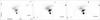 |
Fig. 1 JHKs broadband emission. |
In a previous paper (Paron et al. 2014; hereafter Paper I) we presented results from the observation of highly misaligned molecular outflows toward the infrared (IR) point source UGPS J185808.46+010041.8 (Lucas et al. 2008; UKIDSS Consortium 2012). Analyzing public UKIDSS near-IR data (JHKs broadbands) extracted from the WFCAM Science Archive, we found some diffuse emission showing a cone-like nebula related to the point source, which could be due to a cavity cleared in the circumstellar material by a precessing jet. This source, located at a distance of about 1.1 kpc (Lumsden et al. 2013), was suggested to be a young intermediate-mass protostar (about 3 M⊙) from a spectral energy distribution (SED) analysis (Paper I).
To study the origins of the misalignment in the molecular outflows and the possibility of a precessing jet, we obtained high-resolution images of this source with NIRI at the Gemini Telescope, using a set of broad- and narrowband near-IR filters.
2. Observations and data reduction
In this study we analyze several near-IR broad- and narrowband images (see Table 1) toward the source UGPS J185808.46+010041.8 (hereafter IRS). The images were acquired with NIRI, the Near InfraRed Imager and Spectrometer (Hodapp et al. 2003) at the Gemini-North 8.2 m telescope. The observations were carried out during August and October 2014 and April 2015 in queue mode (Band-1 Program GN-2014B-Q-35). NIRI was used with the f/6 camera, which provides a plate scale of 0.̋117 pix-1 in a field of view of 120′′ × 120′′.
To optimize telescope time, the images were performed following a dither pattern in which the offset directions and amplitudes were selected to be able to perform the near-IR background correction using the on-source images. For the dither pattern, particular careful was taken to avoid contaminating the IRS source and its associated nebular emission by a saturated field star that is located at about 30 arcsec from the IRS source, whose residuals inevitably remain in subsequent images.
For data reduction NIRI images were first passed through nirlin.py, a Python script provided by the Gemini Observatory that applies a per-pixel linearity correction. All subsequent processes such as background correction, image co-addition, and astrometric solution were performed with Theli (Schirmer 2013; Erben et al. 2005). For the absolute astrometric solution, stars in the field of the 2MASS 6X Point Source Working Database Catalog (Cutri et al. 2012) were used.
Table 1 lists the filters used with their central wavelength and width, the effective spatial resolution measured as the average FWHM of point sources in the final co-added images, the number of individual frames, and the effective exposure times of the final co-added images. All images were later normalized to 1 s.
The H-cont image was used to subtract the continuum of [FeII] and the K-cont image to subtract the continuum of H2 1−0 S(1), Brγ, H2 2−1 S(1), and CO 2−0 (bh). For the continuum subtraction the images were convolved with an elliptical Gaussian function using the gauss IRAF1 task to achieve a similar PSF for the point sources in the central area of both images. In this process the effective resolution of both images was degraded to a similar value. After convolution the images were scaled to account for the differences in filter width and throughput, and other effects derived from observing conditions in different nights (both instrumental and environmental). An initial scale factor was derived from aperture photometry of point sources in the central part of the field, this value was checked to agree with the values derived from the ratio of filter transmissions. The initial scale factors were later fine-tuned by visual inspection of the residuals in subtracted images. The object nebular emission in all the subtracted images is above 5σ over the background.
Near-IR bands observed with NIRI at the Gemini-North.
3. Results
Figure 1 displays in three panels the emission of the JHKs broadbands obtained toward IRS. This shows in great detail a nebula extending to the north/northeast of the point source, which appears to be attached to IRS by a jet-like structure. The nebula is mainly composed of two arc-like features; the feature closer to the source is more intense than the feature farther away, which is more extended and diffuse. In the three bands the nebula connected with the jet-like structure is resolved into a twisted-shaped feature. In addition, the emission at the Ks band presents a noteworthy bow-shock-like structure to the northeast. Figure 2 displays in a three-color image the JHKs bands where these structures in the three bands are superimposed. It is worth noting that these images improve in resolution and sensitivity on the JHKs images from UKIDSS presented in Paper I, which is one of the best near-IR images set obtained toward this type of nebula related to intermediate and high-mass YSOs presented to date.
Figure 3 presents the continuum emission at the observed narrowbands H and Ks, while Fig. 4 displays the narrowband images centered on the emission lines of [FeII], H2 1−0 S(1), H2 2−1 S(1), Brγ, and CO 2−0 (bh), with and without continuum (left and right panels, respectively). As expected, the images of the narrowband filters with the continuum show diffuse emission with a similar morphology as observed in the broadband images, while some features and knots that are most likely due to the pure line emission are more evident in the narrowband images. The continuum-subtracted images show that the [FeII] emission presents two bright knots at the end of the jet-like structure that extends from the stellar source to the closer arc-like feature. These knots are located at a projected distance of 2.8 and 1.7 arcsecs from IRS (~0.015 and 0.009 pc, respectively, at the assumed distance of 1.1 kpc). In the close vicinity of IRS, the H2 1−0 S(1) line shows several knots located at different distances, most of them lying at the arc-like feature closer to IRS (located at the projected distance of about 3.2 arcsecs, i.e., ~0.017 pc from IRS), then a bow-shock feature composed of two arc-like structures at a projected distance of 5.5 arcsecs (~0.03 pc) from IRS, and finally an isolated and farthest knot toward the northeast at a projected distance of 7.4 arcsecs (~0.04 pc) from the stellar source. The morphology of the H2 2−1 S(1) emission resembles that of the lower transition, presenting the same features in the close vicinity of IRS, but fainter. The CO 2−0 (bh) line shows diffuse emission composed of two structures located at the arc-like feature closer to IRS, although these structures have to be taken with caution because the CO 2−0 (bh) emission shape was sensitive to the parameters chosen for the continuum subtraction. Finally, the Brγ line also presents some diffuse emission with a peak slightly shifted with respect to the westernmost CO structure.
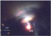 |
Fig. 2 Three-color image with the JHKs broadband emission presented in blue, green, and red, respectively. |
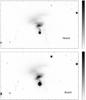 |
Fig. 3 Narrowband H and K continuum in the upper and bottom panels, respectively. White and black in the color bars represent 0% and 100% of the emission, and the highest values are 3 and 30 ADU for the H- and K-cont emission, respectively. All images were normalized to 1 s. |
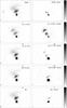 |
Fig. 4 Left panels: narrowband images centered on the indicated lines with continuum. Right panels: narrowband images centered on the indicated lines where the corresponding continuum was subtracted. The object nebular emission in all the subtracted images is above 5σ over the background. White and black in the color bars represent 0% and 100% of the emission. The highest values are (from top to bottom panel) 3, 35, 10, 15, and 10 ADU. All images were normalized to 1 s. |
To compare the emission-line features along the cone-shaped nebula, we performed a similar analysis as in Davis et al. (2011). In Fig. 5 we present the profiles of [FeII], H2 1−0 and 2−1 S(1) (top panel), and CO 2−0 (bh) and Brγ (bottom panel). In both plots the continuum emission in the K band, observed with the K-cont filter, is included for comparison. These profiles were generated by integrating the emissions along a line perpendicular to the cone axis across the whole extension of the cone-shaped nebula. As the H2 1−0 S(1) extends in knots and filaments much farther than the other emission lines (see below), for its profile plot we only included the emission found in the close vicinity of IRS. Table 2 shows the peak positions of each observed feature obtained from Gaussian fits to the profiles presented in Fig. 5. The errors from the Gaussian fits are about 10%, which in most of the cases are values lower than the effective spatial resolution of the observations.
This analysis shows that the emission lines profiles (except the H2 1−0 S(1)) peak with the highest intensity at the position of the IRS source. In similar way, all the emission lines have a second peak between 2 and 3 arcsec offset. A third emission peak is located at about 6 arcsec offset, but only for H2 1−0 S(1) and H2 2−1 S(1). These last two emission peaks are generated by the two arc-like features that are clearly displayed in the 2D images. An inspection of the 2D images shows that the second peak in the [FeII] profile is generated by projected blend of the profiles of more compact knots (in contrast with the more diffuse nebula of Brγ and H2 lines). As mentioned before, the two H2 emission lines that trace low-excitation regions extend beyond being interesting to note here the case of H2 1−0 S(1), for which the projected emission increases with the distance to the source. It is important to note that any comparison with the equivalent analysis presented in Davis et al. (2011) should be done with care because the two studies are applied to sources of different mass, Davis and collaborators studied Herbig-Haro-type outflow sources.
To study the excitation conditions of the H2 lines, we obtained the intensity ratio between the H2 S(1) 1−0 and H2 S(1) 2−1 lines toward the three H2 structures defined in Fig. 5, whose offset on the sky from IRS is shown in Table 2. The obtained values are about 10 for the first arc-like feature (first peak of the H2 profiles in Fig. 5), and ~25 for the second arc-like feature (second peak in Fig. 5) and for the isolated and farthest knot (third tiny peak in the same figure). In Sect. 4.1 we discuss these.
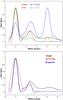 |
Fig. 5 Profiles of the line emission plotted along the axis of the cone-shaped nebula (the offset axis is measured in the plane of the sky). In the top panel we present profiles of [FeII], H2 1−0 S(1), and H2 2−1 S(1) in red, blue, and green, respectively. In the bottom panel we show the profiles of CO 2−0 (bh) and Brγ in red and blue, respectively. In both panels, the continuum emission in K band, observed with the K-cont filter (black), is included for comparison. The profiles are normalized to the peak emission. |
Finally, we inspected the images to search for emission that might be related to IRS at larger spatial scales. The only case in which emission extends beyond the emission localized in the close vicinity of IRS is in H2 1−0 S(1). In the H2 1−0 S(1) continuum-subtracted image several knots and filaments appear at about 45′′ (equivalent to 49.5 kAU in projection) around IRS toward the northwest and southwest, which perfectly match the distribution of the red- and blueshifted molecular outflows discovered in Paper I. Figure 6 shows the H2 1−0 S(1) continuum-subtracted emission with contours of the integrated 12CO J = 3−2 line as presented in Paper I.
3.1. Proper motions
Following the precessing jet scenario and using two observations with temporal difference, it is possible to estimate the proper motions of some structure belonging to the cone-shaped nebula. To do so, we compared our J-band observations of the field, taken in August 2014, with the J-band image from the UKIDSS Survey taken in June 2005, providing a temporal interval of about nine years. The angular resolutions are about 0.1 and 0.4 arcsec pix-1 for Gemini and UKIDSS, respectively. The astrometry of the two images was checked based on the position of several point sources in the field, and no evident offset was detected within the resolutions involved.
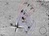 |
Fig. 6 H2 1−0 S(1) continuum-subtracted emission with the 12CO J = 3−2 contours superimposed, as presented in Paper I, representing the red- and blueshifted molecular outflows. The yellow cross is the IRS position and the beam-size of the 12CO observations is shown in the bottom right corner. |
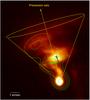 |
Fig. 7 Combination of the J-band emission obtained in two different epochs: the background image is from our observations obtained in 2014, while the green superimposed contours are from the UKIDSS Survey image obtained in 2005. The green and black crosses are the peak positions in 2005 and 2014, respectively, of the same clump-like feature related to the jet. |
Figure 7 shows in the background the J-band emission obtained from our observations, and the J-band emission from the UKIDSS Survey superimposed in green contours. Based on the morphology of the emission, we delineate the cone that is probably traced by the precessing jet (in yellow). The proper motion of the jet can be roughly characterized based on the assumption that the jet is moving onto the cone wall. In Fig. 7 the shift in the emission structure can be assessed by comparing a clump-like feature, whose peak position is indicated with a green cross for 2005, and with a black cross for 2014. Assuming that this feature is moving onto the cone wall, the spatial projected shift of 0.95 arcsec can be decomposed into two components. One component, perpendicular to the cone axis, is related to the jet precession movement, of about 0.80 arcsec (green dashed line) and the other component, in vertical direction along the cone wall, is associated with the ejection movement, of about 0.51 arcsec (black dashed line). Considering that the clump-like feature has taken about nine years to cover the distance represented by the green dashed line, we estimate that it would take about 150 yr to cover the perimeter of the green circumference shown in Fig. 7 (precession period). Considering the other component of the proper motion represented by the black dashed line, we estimate an ejection velocity of about 200 km s-1 for the jet (a lower limit given possible projection effects not considered here), which agrees well with typical jet axial speeds from the literature (100–400 km s-1) (Mundt et al. 1990; Konigl & Pudritz 2000). Using these parameters and following Weigelt et al. (2006) and Smith & Rosen (2005), we can roughly analyze whether the jet precession period is slow or fast. To do this, it is necessary to compare the jet precession period with the outflow expansion time. This parameter is proportional to the jet dynamical time tj = rj/vj and the ratio of jet to ambient density, η = ρj/ρa, being rj and vj the initial jet radius and speed. Additionally, it is inversely proportional to sin(θ), where θ is the half-angle of the precession cone. Using vj = 200 km s-1 and θ = 35°, and assuming rj = 1.7 × 1015 cm and η = 10 (Smith & Rosen 2005), we obtain an outflow expansion timescale of about 50 yr. This means that because the jet precession period was estimated to be 150 yr, three times longer than the outflow expansion timescale, this probably is a slowly precessing jet. As Smith & Rosen (2005) pointed out, the slowly precessing jets generate helical flows, which agrees with the observed near-IR emission morphology.
4. Discussion
The cone-shaped nebula observed in the JHKs broadbands points to the northeast of IRS, opening in a wide angle of about 70°. This near-IR emission most likely arises from a cavity cleared in the circumstellar material and may be due to a combination of different emitting processes: radiation from the central protostar that is scattered at the inner walls of the cavity, emission from warm dust, and line emission from [FeII] and shock-excited H2, among other emission lines (e.g., Reipurth et al. 2000; Bik et al. 2005, 2006). As shown in Fig. 4, some of these lines were detected. Additionally, the curved morphology of the jet-like feature and the twisted-shaped nebula, mainly observed in the J-band, strongly suggests a precessing jet. Models presented in Smith & Rosen (2005) showed that the dominant structure produced by a precessing jet is an inward-facing cone, and particularly, a slowly precessing jet leads to helical flows, generating a spiral-shaped nebula. From our analysis of proper motions (see Sect. 3.1), we not only prove the existence of a precessing jet driven by IRS, but also that the precessing movement is slow (precession period = 150 yr), giving strong observational support to the numerical models of Smith & Rosen (2005).
4.1. Emission-line features
For comparison, the observed emission lines are presented in color-composed images in Fig. 8, which displays in the top panel the continuum-subtracted CO 2−0 (bh), H2 1−0 S(1), and [FeII], in the middle panel the continuum-subtracted Brγ, H2 1−0 S(1), and [FeII], and in the bottom panel the continuum-subtracted CO 2−0 (bh) and Brγ. It is known that the [FeII] emission traces the innermost part of jets that are accelerated near the driving source (Reipurth et al. 2000). The [FeII] is closely related to emission knots and shock fronts along the jet axis, tracing a high-velocity (v ~ 50−200 km s-1), hot (T ~ 104 K), dense (electron densities ~105 cm-3), and partially ionized region (Bally et al. 2007; Davis et al. 2011). The H2 emission around YSOs usually delineates a slow (v ~ 10−30 km s-1), low-excitation, shocked molecular gas component (T ~ 2 × 10³ K, n ≥ 103 cm-3) (Bally et al. 2007; Davis et al. 2011). In addition to the collisional excitation mechanism, another possible mechanism might excite the H2 emission that should be considered: the UV fluorescence. One way to distinguish between the collisional and radiative mechanisms is through the H2 S(1) 1−0/2−1 ratio. In the collisional case, high ratios (about 10) are expected, while the radiative mechanism produces lower ratios (about 2) (e.g., Black & van Dishoeck 1987; Wolfire & Konigl 1991; Smith 1995). The H2 S(1) 1−0/2−1 ratio analysis toward the features observed in the close vicinity of IRS shows that they are indeed produced by shocked gas, that is, the H2 emission is collisionally excited. Moreover, taking into account that in the closer arc-like feature the [FeII] and H2 emissions are spatially coincident (see Fig. 8, upper and middle panels), we suggest that this feature may be produced by a J shock in which the [FeII] emission arises in regions where the shock velocity could be higher than 30 km s-1, while the H2 emission is originated in regions where the shock velocity is slower than 25 km s-1 and the molecule is not dissociated (Hollenbach & McKee 1989; Smith 1994; Reipurth et al. 2000), or in the post-shock cooling region, where the molecules reform and radiate. Thus, even though a J shock can be dissociative, emission from H2 lines may be detected. In addition, it is important to keep in mind that iron can also be excited in C shocks (Dionatos et al. 2013, 2014). On the other hand, regions with H2 emission without [FeII] can be explained by both a nondissociated C shock or a less energetic J shock (Hollenbach & McKee 1989; Dionatos et al. 2013, 2014). This is the case of the second arc-like feature in the vicinity of IRS and the H2 1−0 S(1) features observed in the larger spatial scale shown in Fig. 6. As observed in the figure, these features perfectly correlate with the 12CO outflows presented in Paper I, showing shocked molecular gas along them, and confirming its nature of molecular outflows.
The CO bandheads are excited in hot and very dense regions ( T> 2000 K and n> 1010 cm-3), physical conditions that can be found in accretion disks (Scoville et al. 1983; Carr 1989; Bik & Thi 2004), neutral winds (Carr 1989), and funnel flows between the disk and the central source (Martin 1997). There is an intriguing aspect of the Brγ emission around IRS: on one hand, Brγ is excited at very high temperatures (T ~ 104 K) and its emission usually spatially correlates with that of the CO 2−0 (bh) in YSO environments (Ilee et al. 2014, and references therein), which is not the case of IRS (see Fig. 8 bottom panel). Moreover, according to Kumar et al. (2003), the Brγ emission can arise in fast J shocks within an envelope of thousands of AU surrounding the young star. If this were the case of IRS, then it is expected that the Brγ emission would correlate with the [FeII] emission, which is also not the case of IRS (see Fig. 8 middle panel). We suggest that the Brγ emission is probably associated with stellar wind (Kraus et al. 2008).
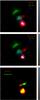 |
Fig. 8 Color images composed with the continuum-subtracted lines indicated in each panel. The black and the respective color in the color bars represents 0% and 100% of emission. The highest values are 8, 50, and 2 ADU for red, green, and blue, respectively, in the top and middle panels, and 5 ADU for red and green in the bottom panel. All images were normalized to 1 s. |
4.2. Orientation of the observed circumstellar structures
We dedicate this section to discuss some aspects of the puzzling orientation of the molecular outflows detected in 12CO J = 3−2 and H2 1−0 S(1) lines, compared with that of the jet, the arclike features, and knots observed in the near-IR lines.
As shown in Paper I and reinforced in this study through the H2 1−0 S(1) extended emission, which maps shocked molecular gas, the molecular outflows are indeed highly misaligned. The redshifted outflow points toward the northwest, while the blueshifted outflow points toward the southwest. Concerning the near-IR features in the close environment of IRS, as observed toward other similar sources (see Preibisch et al. 2003; Massi et al. 2004; Kraus et al. 2006; Weigelt et al. 2006; Paron et al. 2013) the nebula, with a cone shape and arc-like features, extends only to one side. To justify this unidirectional asymmetry, it has previously been proposed that the observed near-IR features might be related to a blueshifted jet with the redshifted counterpart not detected in the near-IR bands because they are more highly extinct. When molecular outflows were observed through molecular rotational transitions, the nebula observed in the near-IR images matched the orientation and alignment of blueshifted molecular outflows. In the case presented here, it is puzzling that the blueshifted molecular outflow points toward the southwest and the observed cone shape nebula with arc-like features toward the northeast. It may suggest that they are not related, or that a complex relation exists that is not evidenced in these images because of the large difference in the angular resolution between the millimeter and near-IR data. One possibility might be that we observe an unresolved system of YSOs. At the assumed distance of 1.1 kpc, the spatial resolution presented here is about 400 AU. It is known that a region of this size, or even smaller, can contain a binary system (Connelley et al. 2008). In an scenario with more than one YSO, a complex (and so far unusual when compared with low-mass YSO outflow studies) distribution of jets and molecular outflows can be expected, as might be the case for IRS. In this way, the existence of a precessing jet may be explained through tidal interactions between companion stars.
Additionally, by inspecting the 12CO J = 3−2 distribution, we note that the peak of the blueshifted component coincides in projection with IRS. This shows that the 12CO J = 3−2 emission around IRS is predominantly blueshifted, which would relate the near-IR cone-shaped nebula to blueshifted gas. This agrees with a scenario of more than one YSO, where the blueshifted 12CO J = 3−2 peaking at IRS and the lobe extending toward the southwest are produced by different sources. Interferometric rotational lines CO observations are required to resolve the molecular outflow morphology.
5. Summary and concluding remarks
In Paper I we reported misaligned molecular outflows toward the intermediate-mass YSO UGPSJ185808.46+010041.8 (IRS), and based on public near-IR data, we suggested the presence of a precessing jet. To study this interesting source in more detail, we presented here the results derived from a new high-resolution image set obtained with the Gemini-NIRI in the JHKs broadbands and [FeII], H2 1−0 (S1), Brγ, H2 2−1 (S1), and CO 2−0 (bh) narrowbands.
The near-IR imaging toward IRS, obtained with a spatial resolution of about 400 AU at the assumed distance of 1.1 kpc, strongly suggest a precessing jet. The observed cone-shaped nebula composed of a twisted-shaped feature with two arc-like structures is one of the best images of this type of objects presented to date. These images give an important observational support to the models that point out that precessing jets generate this type of near-IR features in massive YSOs. An analysis of proper motions based on our Gemini observations and UKIDSS data additionally supports the precession scenario and allowed us to estimate a precession period of 150 yr, a jet axial speed of about 200 km s-1, and an outflow expansion timescale of about 50 yr. These parameters suggest a slow-precessing jet, which, as shown by models presented in Smith & Rosen (2005), leads to helical flows in agreement with the structures observed in our near-IR images.
The analysis of the observed near-IR lines showed that the H2 is collisionally excited, and the spatial coincidence of the [FeII] and H2 emissions in the closer arc-like feature suggests that this region can be affected by a J shock. However, it is important to keep in mind that iron can also be excited in C shocks. The second arc-like feature presents H2 emission without [FeII], which could be explained by nondissociated C shock or a less energetic J shock, as is the case of the H2 1−0 S(1) features observed on a larger spatial scale. In the H2 1−0 S(1) continuum-subtracted image, the only case in which near-IR emission was detected to extend beyond the localized in the IRS close vicinity, several knots and filaments appear that perfectly match the distribution of the molecular outflows discovered in Paper I, confirming shocked gas within the outflow lobes. Finally, we suggest that the Brγ emission around IRS probably arises from stellar winds.
The orientation of the molecular outflows is puzzling (the redshifted outflow points toward the northwest and the blueshifted outflow toward the southwest), compared with the near-IR features (which point toward the northeast). One possibility is an unresolved system of YSOs. The 12CO J = 3−2 emission around IRS is predominantly blueshifted, which suggests a relation between the near-IR cone-shaped nebula and the blueshifted gas. In this case, the blueshifted 12CO J = 3−2 peaking at IRS and the lobe extending toward the southwest might be produced by different sources. This scenario can explain the precessing jet through tidal interactions between companion stars. Interferometric rotational lines CO observations are required to resolve the molecular outflow morphology.
Acknowledgments
We thank the anonymous referee for the helpful comments and suggestions. The authors are very grateful to the Gemini staff for their dedication and helpful support in carrying out our observational program. S.P. and M.O. are members of the Carreradel Investigador Científico of CONICET, Argentina. This work was partially supported by Argentina grants awarded by UBA (UBACyT), CONICET and ANPCYT.
References
- Bally, J., Reipurth, B., & Davis, C. J. 2007, Protostars and Planets V, 215 [Google Scholar]
- Bally, J., Walawender, J., Reipurth, B., & Megeath, S. T. 2009, AJ, 137, 3843 [NASA ADS] [CrossRef] [Google Scholar]
- Bally, J., Youngblood, A., & Ginsburg, A. 2012, ApJ, 756, 137 [NASA ADS] [CrossRef] [Google Scholar]
- Bik, A., & Thi, W. F. 2004, A&A, 427, L13 [NASA ADS] [CrossRef] [EDP Sciences] [Google Scholar]
- Bik, A., Kaper, L., Hanson, M. M., & Smits, M. 2005, A&A, 440, 121 [NASA ADS] [CrossRef] [EDP Sciences] [Google Scholar]
- Bik, A., Kaper, L., & Waters, L. B. F. M. 2006, A&A, 455, 561 [NASA ADS] [CrossRef] [EDP Sciences] [Google Scholar]
- Black, J. H., & van Dishoeck, E. F. 1987, ApJ, 322, 412 [NASA ADS] [CrossRef] [Google Scholar]
- Carr, J. S. 1989, ApJ, 345, 522 [NASA ADS] [CrossRef] [Google Scholar]
- Ciardi, A., & Hennebelle, P. 2010, MNRAS, 409, L39 [NASA ADS] [Google Scholar]
- Connelley, M. S., Reipurth, B., & Tokunaga, A. T. 2008, AJ, 135, 2496 [NASA ADS] [CrossRef] [Google Scholar]
- Cutri, R. M., Skrutskie, M. F., van Dyk, S., et al. 2012, VizieR Online Data Catalog: II/281 [Google Scholar]
- Davis, C. J., Cervantes, B., Nisini, B., et al. 2011, A&A, 528, A3 [NASA ADS] [CrossRef] [EDP Sciences] [Google Scholar]
- Dionatos, O., Jørgensen, J. K., Green, J. D., et al. 2013, A&A, 558, A88 [NASA ADS] [CrossRef] [EDP Sciences] [Google Scholar]
- Dionatos, O., Jørgensen, J. K., Teixeira, P. S., Güdel, M., & Bergin, E. 2014, A&A, 563, A28 [NASA ADS] [CrossRef] [EDP Sciences] [Google Scholar]
- Erben, T., Schirmer, M., Dietrich, J. P., et al. 2005, Astron. Nachr., 326, 432 [NASA ADS] [CrossRef] [Google Scholar]
- Hodapp, K. W., Jensen, J. B., Irwin, E. M., et al. 2003, PASP, 115, 1388 [NASA ADS] [CrossRef] [Google Scholar]
- Hollenbach, D., & McKee, C. F. 1989, ApJ, 342, 306 [NASA ADS] [CrossRef] [Google Scholar]
- Ilee, J. D., Fairlamb, J., Oudmaijer, R. D., et al. 2014, MNRAS, 445, 3723 [NASA ADS] [CrossRef] [Google Scholar]
- Konigl, A., & Pudritz, R. E. 2000, Protostars and Planets IV, 759 [Google Scholar]
- Kraus, S., Balega, Y., Elitzur, M., et al. 2006, A&A, 455, 521 [NASA ADS] [CrossRef] [EDP Sciences] [Google Scholar]
- Kraus, S., Hofmann, K.-H., Benisty, M., et al. 2008, A&A, 489, 1157 [NASA ADS] [CrossRef] [EDP Sciences] [Google Scholar]
- Kumar, M. S. N., Fernandes, A. J. L., Hunter, T. R., Davis, C. J., & Kurtz, S. 2003, A&A, 412, 175 [NASA ADS] [CrossRef] [EDP Sciences] [Google Scholar]
- Lefloch, B., Cernicharo, J., Reipurth, B., Pardo, J. R., & Neri, R. 2007, ApJ, 658, 498 [NASA ADS] [CrossRef] [Google Scholar]
- Lewis, B. T., Bate, M. R., & Price, D. J. 2015, MNRAS, 451, 288 [NASA ADS] [CrossRef] [Google Scholar]
- Lucas, P. W., Hoare, M. G., Longmore, A., et al. 2008, MNRAS, 391, 136 [NASA ADS] [CrossRef] [Google Scholar]
- Lumsden, S. L., Hoare, M. G., Urquhart, J. S., et al. 2013, ApJS, 208, 11 [NASA ADS] [CrossRef] [Google Scholar]
- Martin, S. C. 1997, ApJ, 478, L33 [NASA ADS] [CrossRef] [Google Scholar]
- Massi, F., Codella, C., & Brand, J. 2004, A&A, 419, 241 [NASA ADS] [CrossRef] [EDP Sciences] [Google Scholar]
- McKee, C. F., & Ostriker, E. C. 2007, ARA&A, 45, 565 [NASA ADS] [CrossRef] [Google Scholar]
- Mundt, R., Buehrke, T., Solf, J., Ray, T. P., & Raga, A. C. 1990, A&A, 232, 37 [NASA ADS] [Google Scholar]
- Paron, S., Fariña, C., & Ortega, M. E. 2013, A&A, 559, L2 [NASA ADS] [CrossRef] [EDP Sciences] [Google Scholar]
- Paron, S., Ortega, M. E., Petriella, A., & Rubio, M. 2014, A&A, 567, A99 [NASA ADS] [CrossRef] [EDP Sciences] [Google Scholar]
- Preibisch, T., Balega, Y. Y., Schertl, D., & Weigelt, G. 2003, A&A, 412, 735 [NASA ADS] [CrossRef] [EDP Sciences] [Google Scholar]
- Reipurth, B., & Bally, J. 2001, ARA&A, 39, 403 [NASA ADS] [CrossRef] [Google Scholar]
- Reipurth, B., Yu, K. C., Heathcote, S., Bally, J., & Rodríguez, L. F. 2000, AJ, 120, 1449 [NASA ADS] [CrossRef] [Google Scholar]
- Reiter, M., Smith, N., Kiminki, M. M., Bally, J., & Anderson, J. 2015, MNRAS, 448, 3429 [NASA ADS] [CrossRef] [Google Scholar]
- Schirmer, M. 2013, ApJS, 209, 21 [NASA ADS] [CrossRef] [Google Scholar]
- Scoville, N., Kleinmann, S. G., Hall, D. N. B., & Ridgway, S. T. 1983, ApJ, 275, 201 [NASA ADS] [CrossRef] [Google Scholar]
- Smith, M. D. 1994, MNRAS, 266, 238 [NASA ADS] [CrossRef] [Google Scholar]
- Smith, M. D. 1995, A&A, 296, 789 [NASA ADS] [Google Scholar]
- Smith, M. D., & Rosen, A. 2005, MNRAS, 357, 579 [NASA ADS] [CrossRef] [Google Scholar]
- UKIDSS Consortium 2012, VizieR Online Data Catalog: II/316 [Google Scholar]
- Weigelt, G., Beuther, H., Hofmann, K.-H., et al. 2006, A&A, 447, 655 [NASA ADS] [CrossRef] [EDP Sciences] [Google Scholar]
- Wolfire, M. G., & Konigl, A. 1991, ApJ, 383, 205 [NASA ADS] [CrossRef] [Google Scholar]
All Tables
All Figures
|
Fig. 1 JHKs broadband emission. |
| In the text | |
|
Fig. 2 Three-color image with the JHKs broadband emission presented in blue, green, and red, respectively. |
| In the text | |
|
Fig. 3 Narrowband H and K continuum in the upper and bottom panels, respectively. White and black in the color bars represent 0% and 100% of the emission, and the highest values are 3 and 30 ADU for the H- and K-cont emission, respectively. All images were normalized to 1 s. |
| In the text | |
|
Fig. 4 Left panels: narrowband images centered on the indicated lines with continuum. Right panels: narrowband images centered on the indicated lines where the corresponding continuum was subtracted. The object nebular emission in all the subtracted images is above 5σ over the background. White and black in the color bars represent 0% and 100% of the emission. The highest values are (from top to bottom panel) 3, 35, 10, 15, and 10 ADU. All images were normalized to 1 s. |
| In the text | |
|
Fig. 5 Profiles of the line emission plotted along the axis of the cone-shaped nebula (the offset axis is measured in the plane of the sky). In the top panel we present profiles of [FeII], H2 1−0 S(1), and H2 2−1 S(1) in red, blue, and green, respectively. In the bottom panel we show the profiles of CO 2−0 (bh) and Brγ in red and blue, respectively. In both panels, the continuum emission in K band, observed with the K-cont filter (black), is included for comparison. The profiles are normalized to the peak emission. |
| In the text | |
|
Fig. 6 H2 1−0 S(1) continuum-subtracted emission with the 12CO J = 3−2 contours superimposed, as presented in Paper I, representing the red- and blueshifted molecular outflows. The yellow cross is the IRS position and the beam-size of the 12CO observations is shown in the bottom right corner. |
| In the text | |
|
Fig. 7 Combination of the J-band emission obtained in two different epochs: the background image is from our observations obtained in 2014, while the green superimposed contours are from the UKIDSS Survey image obtained in 2005. The green and black crosses are the peak positions in 2005 and 2014, respectively, of the same clump-like feature related to the jet. |
| In the text | |
|
Fig. 8 Color images composed with the continuum-subtracted lines indicated in each panel. The black and the respective color in the color bars represents 0% and 100% of emission. The highest values are 8, 50, and 2 ADU for red, green, and blue, respectively, in the top and middle panels, and 5 ADU for red and green in the bottom panel. All images were normalized to 1 s. |
| In the text | |
Current usage metrics show cumulative count of Article Views (full-text article views including HTML views, PDF and ePub downloads, according to the available data) and Abstracts Views on Vision4Press platform.
Data correspond to usage on the plateform after 2015. The current usage metrics is available 48-96 hours after online publication and is updated daily on week days.
Initial download of the metrics may take a while.