| Issue |
A&A
Volume 593, September 2016
|
|
|---|---|---|
| Article Number | A106 | |
| Number of page(s) | 14 | |
| Section | Stellar structure and evolution | |
| DOI | https://doi.org/10.1051/0004-6361/201628411 | |
| Published online | 30 September 2016 | |
Short-term variability and mass loss in Be stars
II. Physical taxonomy of photometric variability observed by the Kepler spacecraft
1 ESO – European Organisation for Astronomical Research in the Southern Hemisphere, Casilla 19001, Santiago 19, Chile
e-mail: This email address is being protected from spambots. You need JavaScript enabled to view it.
2 ESO – European Organisation for Astronomical Research in the Southern Hemisphere, Karl-Schwarzschild-Str. 2, 85748 Garching, Germany
e-mail: This email address is being protected from spambots. You need JavaScript enabled to view it.
3 Instituto de Astronomia, Geofísica e Ciências Atmosféricas, Universidade de São Paulo, 05508-900 São Paulo, SP, Brazil
Received: 29 February 2016
Accepted: 2 August 2016
Abstract
Context. Classical Be stars have been established as pulsating stars. Space-based photometric monitoring missions contributed significantly to that result. However, whether Be stars are just rapidly rotating SPB or β Cep stars, or whether they have to be understood differently, remains debated in the view of their highly complex power spectra.
Aims. Kepler data of three known Be stars are re-visited to establish their pulsational nature and assess the properties of additional, non-pulsational variations. The three program stars turned out to be one inactive Be star, one active, continuously outbursting Be star, and one Be star transiting from a non-outbursting into an outbursting phase, thus forming an excellent sample to distill properties of Be stars in the various phases of their life-cycle.
Methods. The Kepler data was first cleaned from any long-term variability with Lomb-Scargle based pre-whitening. Then a Lomb-Scargle analysis of the remaining short-term variations was compared to a wavelet analysis of the cleaned data. This offers a new view on the variability, as it enables us to see the temporal evolution of the variability and phase relations between supposed beating phenomena, which are typically not visualized in a Lomb-Scargle analysis.
Results. The short-term photometric variability of Be stars must be disentangled into a stellar and a circumstellar part. The stellar part is on the whole not different from what is seen in non-Be stars. However, some of the observed phenomena might be to be due to resonant mode coupling, a mechanism not typically considered for B-type stars. Short-term circumstellar variability comes in the form of either a group of relatively well-defined, short-lived frequencies during outbursts, which are called Štefl frequencies, and broad bumps in the power spectra, indicating aperiodic variability on a time scale similar to typical low-order g-mode pulsation frequencies, rather than true periodicity.
Conclusions. From a stellar pulsation perspective, Be stars are rapidly rotating SPB stars, that is they pulsate in low order g-modes, even if the rapid rotation can project the observed frequencies into the traditional high-order p-mode regime above about 4 c/d. However, when a circumstellar disk is present, Be star power spectra are complicated by both cyclic, or periodic, and aperiodic circumstellar phenomena, possibly even dominating the power spectrum.
Key words: circumstellar matter / stars: emission-line, Be / stars: oscillations / stars: activity
© ESO, 2016
1. Introduction
Classical Be stars are rapidly rotating B stars, surrounded by a self-ejected gaseous disk, the evolution of which is governed by viscosity. As a class, they are known to pulsate in non-radial modes, but not to harbor large scale magnetic fields (see Rivinius et al. 2013, for a review). In general, Be stars and their disks could be considered as fairly well understood, was it not for the one central question that is still open: how are these disks formed? The physical mechanism ejecting matter from the stellar surface with sufficient energy and angular momentum to form a Keplerian disk, sometimes called the Be phenomenon, remains elusive.
There is evidence that this Be phenomenon, at least in some stars, is related to non-radial pulsation. This has first been shown by means of spectroscopy in μ Cen (see, e.g., Rivinius et al. 1998), but the observational cost of this finding was high; spectra were taken daily for several months each year over a number of years. Similar data sets obtained for other Be stars suggested similar relations, but not as firm as one would have wished.
With the launch of spacecraft dedicated to obtain photometric time series of stars and stellar fields in the visual domain, it has become possible to take data sets combining high precision with high cadence and very long time base, the same combination that has enabled the spectroscopic break-through. Although these missions are usually designed to search for extra-solar planets or take data for the purpose of asteroseismology, they serve equally well for the analysis of the light variations of Be stars. Since Be stars are instrinsically bright and numerous, almost any field of stars as large as the Kepler one and not too far away from the Galactic plane will host at least some of them.
This series of papers has been inspired by the analysis of Be star photometric data taken with the BRITE Constellation satellites (Weiss et al. 2014), and Baade et al. (2016, called Paper I from here on) present some of the first science results obtained from BRITE Constellation data. Paper I presents the analysis of the BRITE data of η Cen and μ Cen, and much of the findings here are already seen in BRITE data, though due to the lower precision of BRITE, which has 3 cm aperture compared to the 95 cm of the telescope aboard Keplerand a less radiation-hard design, not necessarily with the same confidence. In any case, it became clear that every space-based photometry mission has a partly unique potential, that could, and should, be combined with results from other photometry missions and ground based observations to unravel the mystery of the Be phenomenon.
The unique potential for Be stars observed with the Kepler spacecraft (Koch et al. 2010) is without doubt the time basecombined with precision, four full years of near-continuous observations with a cadence of about half an hour. Be stars benefit in particular because they are variable on a wide range of time scales from hours (and sometimes even minutes, but only in the very high energy domain) to decades. In the literature three Be stars have been published that were observed during the original Kepler mission (Balona et al. 2011; Kurtz et al. 2015).
In the following Sect. 2, these three stars are introduced and the analysis method employed in this work is described, which goes somewhat beyond the methods used in the literature by using not only Lomb-Scargle based Fourier analysis, but as well wavelet analysis. In Sect. 3 the results are presented, which do not contradict, but certainly extend the ones reported in the literature, and the implications and interpretations are discussed in Sect. 4. Finally, the results are put into a generalized picture in Sect. 5, and an outlook for future papers of this series is given.
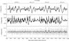 |
Fig. 1 Long-term part of the variability removed by high-pass filtering in black, original data gray in background. For this plot, linear trends have been removed beforehand. Shown are, from top to bottom, ALS 10705, StHα166, and HD 186567. There is a difference in vertical scale, and hence amplitude of the variations. |
2. Targets and analysis methods
Before introducing the targets, some terminology should be made clear. Historically, an “active Be star” was typically understood to be one with emission, but “Be star activity” was often identified with outbursts. This is somewhat inconsistent, and since the understanding of Be stars has reached a level at which this inconsistency becomes an obstacle, it should be resolved. Here and in the following an inactive Be star is one without any detectable disk, while an active Be star has such a disk. This designation is observationally easy to probe, but makes no distinction between stars that currently build a disk and stars in which the disk is decaying, so for the former we introduce the term that it is a disk-feeding Be star. Not withstanding the possibility that a star may build a disk in a continuous manner, that is without outbursts, a star showing repeated and strong outbursts is certainly in a feeding phase,even though in the time span between two successive outbursts the star is not losing mass and the inner disk is technically in a dissipating phase.
2.1. ALS 10705 (KIC 8057661)
ALS 10705 was found to show emission lines by Kohoutek & Wehmeyer (1999). From Kepler data Nielsen et al. (2013) obtain 1.018 d (0.982 c/d) as dominant period, which they attribute to rotation. Two spectra were taken with ESPaDOnS at the CFHT in July 2010, a bit more than a year after the beginning of the Kepler observations. They do not show any line emission. From these spectra, Balona et al. (2011) obtain vsini = 49 ± 5 km s-1, while from Strömgren photometry they derive Teff = 21 kK and log g = 4.2. They give a hybrid SPB and β Cep nature for the pulsational properties and remark that ALS 10705 should be considered as a currently inactive Be star, seen at low inclinationof the rotational axis.
2.2. StHα166 (KIC 6954726)
StHα166 was first noted to be an emission line star by Stephenson (1986) and confirmed to be a Be star by Downes & Keyes (1988). The Kepler Input Catalogue lists an effective temperature of about 17 kK and a log g of 4.8.
Pigulski et al. (2009) identify the star as aperiodic variable in the ASAS photometric database, while based on Kepler observations McNamara et al. (2012) classify the variations as binary or rotational with a dominant frequency of 1.03 c/d, and Reinhold et al. (2013) derive a rotation period of 44.5 d (0.02 c/d). Balona et al. (2011) note the star has frequency groupings, but do not give a physical interpretation and rather mention g-mode pulsation or rotation as possibilities.
Balona et al. also derive vsini = 160 km s-1, again based on two ESPaDOnS spectra, but do not derive other parameters. The spectra are somewhat noisy, but the ratio of He i 4471 vs. Mg ii 4481 does not agree with a temperature as cool as 17 kK, and as well the presence of the Si iii 4553/68/73 triplet confirms that the star must rather be of earlier B subtype. Yet, the absence of He ii lines limits the Teff to lower than about 25 kK.
The Hα emission line was symmetrically double-peaked, at a height of 2.8 in units of the nearby continuum, with a weak central depression, and a total equivalent width of about 13 Å in emission, completely filling in the photospheric wings of Hα. Overall, the spectrum is very typical of an early Be star seen at low to intermediate inclination.
A period analysis for the full 4 yr Kepler data of ALS 10705 and StHα166 has been described by Balona et al. (2015, their Sect. 11). As the first part of the analysis here, a similar technique is employed, the Lomb-Scargle analysis, and the results are the same.
2.3. HD 186567 (KIC 11971405)
HD 186567 is considered as an example for a Be star by Kurtz et al. (2015). The original source of this classification is unclear, but since that the star shows several Be-star typical outbursts (see Fig. 1 vs. Haubois et al. 2012, for a theoretical model how such outbursts produce the observed light curve) there is no strong reason to doubt the classification.
HD 186567 is a late type B star for which Huber et al. (2014) give a temperature of about 12 kK and log g of 3.7. Pigulski et al. (2009) again identify the star as aperiodic variable in ASAS data, while McNamara et al. (2012) classify the variations as hybrid SPB and β Cep showing frequency groups in the Kepler data, with a dominant value of about 4 c/d.
2.4. Light curve preparation
For these three stars all available Kepler data were retrieved from MAST, taken from May 2009 to May 2013 in 18 “quarters”, a term which is used to distinguish observing setups of the satellite. For details see Sect. 4 of Balona et al. (2011) and the references therein. As date the “Barycentric Kepler Julian Date” is used, defined as BKJD = BJD−2 454 833, where BJD = 2 454 833 corresponds to Jan. 1, 2009. All fluxes were converted to a magnitude scale. As data from different quarters may not join smoothly, they were pre-processed for each quarter individually by subtracting a linear trend before merging the quarters into a single data set.
In addition to instrumental trends, and apart from short-term periodic/cyclic variations, which are in the focus of this work, Be stars may show medium to long-term secular variability due to radiative processes (see Haubois et al., op. cit.) in their circumstellar environment. Their gaseous disks form and dissipate on time scales of sometimes weeks, but more often months and even decades. The resulting variability in the visual domain can surpass the amplitude of the short-term variations by as much as three orders of magnitudes in extreme cases. In the three stars under investigation, this ratio is considerably more benign, less than one order of magnitude. For the most variable star in the sample, StHα166, the peak-to-peak amplitude of the secular variations is 0.1 mag, and for the strongest periodic variation it is 0.016 mag.
In terms of data processing it is irrelevant whether such a trend is (partly) stellar or (partly) instrumental; it can be removed in a single step. As a tool for time series analysis the vartools package, published by Hartman et al. (2008)1 is used. The removal of secular trends was implemented as a Fourier-based high-pass filter.
The precise method was to find frequencies in the range between 10-3 and 0.2 c/d with the generalized Lomb-Scargle (LS) periodogram (Zechmeister & Kürster 2009, implemented using Press et al. 1992). These frequencies are removed iteratively by fitting a sinusoid to the actual data (pre-whitening, explicitly without removing harmonics). The iterative removal is conducted at least down to, and mostly beyond the noise level, which is apparent as a frequency continuum in the LS-periodogram. Typically hundreds of frequencies need to be removed before reaching that stage.
A major factor in the applicability of such a method are the aliasing properties of Kepler data, and in fact other space mission data, too: There are no strong peaks of the window function in the range of typical Be star frequencies, which are about 0.5 c/d to about 10 c/d. For this reason, any removal of power at frequencies below 0.2 c/d, that is applying a frequency high-pass filter, does not affect the power spectrum at frequencies of astrophysical interest. Mathematically speaking, therefore, such filtering is not even required; results of the subsequent period search are the same, whether the high-pass filter is applied or not. However, in order to obtain a better visual representation of the secular vs. the periodic behavior (see Fig. 1 for an example), and to fold the data with the obtained periods, the high-pass filter is applied in any case.
Figure 1 shows the original data after removing mean value and linear trends, together with the curve obtained by the high-pass filter (i.e., the sum of all low-frequency terms iteratively found). The variability of StHα166 has strong secular outbursts, while the variations of HD 186567 are dominated by short term variations, which remain in this stage, with only few outbursts towards the end of the observing time span. The variations of ALS 10705 are not obviously identified as either stellar or circumstellar. Recalling the fact that the star was without emission, and considering the rather low amplitude and long time scale of the secular variability, they are likely instrumental effects, also since the pattern roughly repeats annually. If the other stars suffer from a similar pattern, it is hard to see because their variations are dominated by stellar secular variability. In any case, these long-term trends are subtracted in this step, and therefore of no consequence for the results below.
2.5. Light curve analysis
The final analysis is done in two different ways. First, the data are analyzed using the generalized LS periodogram, just as described above, but now in the frequency range of astrophysical interest from 0.2 c/d to 25 c/d; the latter is about the Nyquist frequency of the long cadence data (24.469 c/d). As this method is the traditional way of analyzing such a light-curve, it yields essentially identical results to the ones described by Balona et al. (2011) and Kurtz et al. (2015).
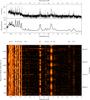 |
Fig. 2 Time series analysis of ALS 10705. From top to bottom the LS periodogram, the time averaged result of the wavelet analysis, both shown in logarithmic scale, and the full 2D result of the wavelet analysis, where the intensity is displayed in logarithmic scale, too. The frequency groups discussed in the text are identified above the lowermost panel. |
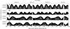 |
Fig. 3 Amplitude variation with time for g1, g8, g4 and g7 (top to bottom) of ALS 10705. The individual points were computed by co-adding the fits to all frequencies found by LS belonging to each group, and then the absolute value was plotted. The upper envelope of each group, therefore, represents the amplitude variations seen in the lower panel of Fig. 2 and illustrates the various correlations described in the text. |
As an alternative way of looking at the data a wavelet analysis is used, again in the implementation included in the vartools package by Hartman et al. (2008), based on Foster (1996, see there also for examples and a critical assessment of the method). In the most simple terms, a wavelet is an oscillating function, here a sinusoid, with a decay term:  (1)where f is the frequency and c a scaling factor of the decay. The decay term is kept constant in units of the frequency, that is the wavelet at any given frequency sees only a fixed number of cycles towards the past and the future; the effective time base of the analysis decreases as frequency increases. As a consequence, the frequency resolution of a wavelet analysis is not a function of the total time base, but one of the frequency sampled: The higher the frequency, the lower the resolution. In this work an unusually slow decay was used. While a standard value is c = 1 / 8π2 ~ 0.0125, here c = 0.0001 was adopted, i.e., coherence over a few hundred instead of just a few oscillations. This was done first since such a rapid change of amplitude and period is not expected, and second to increase the frequency resolution to a level where most of the various groups can be safely disentangled.
For visualization, a 2D representation is used for the result. For any given time step (here: one day) a wavelet periodogram is obtained. All periodograms are then stacked into an image with frequency on the x-axis, time step of the wavelet analysis on the y-axis, and power on the z-axis (the latter coded as intensity in the figures here).
3. Results
Comparison of frequency groups found in the wavelet vs. the dominant frequency of each group found in the LS analysis of ALS 10705.
3.1. ALS 10705
In terms of variability, ALS 10705 is the least complicated object in the sample. Since it is an inactive Be star without any spectroscopic sign of a disk, and even the very low amplitude secular photometric variations are likely to be instrumental, one can be quite certain that there is no circumstellar variability or disk feeding complicating the picture, and therefore all variability detected is photospheric, making ALS 10705 a valuable case to compare variations in other, more active, Be stars to.
First concentrating on the LS periodogram in Fig. 2, one would classify ALS 10705 as a hybrid pulsator, since both low and high frequencies are present, often taken as indicative of g- and p-modes, respectively. We ignore for the moment that such a simple classification is questionable in the case of rapidly rotating objects such as Be stars, where rotation can alter the observed frequencies considerably, and defer this issue to the discussion in Sect. 4.6.
Already in the LS periodogram it can be seen immediately that the variation at about 3.6 and 4.8 c/d cannot be described by a single, stable frequency, but there are a number of peaks, separated in distinct groups. These would normally be interpreted as beating frequencies, that is a number of nearby phase coherent and amplitude stable frequencies that, when co-added to each other, evince the impression of a frequency with variable amplitude, becoming stronger and weaker with a function called the beating envelope. When two individual beating frequencies remain coherent during the sampled time base and are of equal amplitude, the envelope varies strongly between zero and twice the amplitude of an individual frequency. A closer inspection of the frequencies below 2 c/d reveals that the same is the case here, each single peak dissolves to a number of sub-peaks, forming a group of frequencies with a strong beating pattern. Such patterns are seen in Fig. 3, where the absolute values of the co-addedsinusoidal fits to the individual frequencies are shown for several groups,so that the total amplitude and its variations are represented by the upper envelope of each group.
At frequencies lower than 2 c/d increasing noise is seen. When pre-whitening the LS-periodogram, one finds that even after more than 100 iterations significant power still remains in the power spectrum, with clear peaks belonging to one of the above described groups. The identified groups are listed in Table 1.
In the time average of the wavelet transform, these individual groups are not resolved. The decrease of frequency resolution with increasing frequency is obvious, and the residual of the periodic power that has been removed by the high-pass filtering is clearly apparent at frequencies below 0.2 c/d. Except for being of lower quality, however, this plot does not really offer new insight beyond the LS periodogram. Rather than the myriad of peaks seen in the LS periodogram, one can identify individual peaks in the averaged wavelet transform. These correspond to the groups mentioned above (see Fig. 2).
In the full 2D representation of the wavelet analysis, other, and partly different aspects are more easily apparent to the eye. Among other things, the effect of data outliers is easily seen as a sudden, short lived surge of power at all frequencies, akin to the Fourier transform of a δ-function, which displays constant power at all frequencies (see e.g., Fig. 2, lower panel at t = 725). Another difference is scientifically far more interesting. Instead of resolving a frequency group into a high number of single frequencies, that reproduce the over-all behavior of the group by their beating, the wavelet transform sees only a single frequency with variable power. Or, in other words, at the expense of frequency resolution it visualizes the phase and strength of the envelope function of the – supposed – beating, something completely lost in the traditional visualization of a 1D periodogram. This opens the view for new and alternative interpretations.
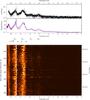 |
Fig. 4 Like Fig. 2, but for StHα166. In the middle panel, instead of the overall wavelet power spectrum, the average power spectrum during more variable phases (t< 700 and 900 <t< 1500) is shown in as a solid line, during less variable (700 <t< 900 and t> 1500) as a dashed one. The label Š denotes the circumstellar Štefl frequencies (see Sect. 4.2). |
Addressing the envelope of the amplitude for each frequency group gi as Ai, Fig. 3 helps to visualize A1, A8, A4, and A7 from top to bottom. The following observations can be made about these envelopes:
-
A1 ~ A8 and
 .
. A1 has minima when either A4 or A7 have a minimum. A1 minima coinciding with A4 minima are deeper than those coinciding with A7 minima.
In Fig. 2 it can as well be seen that A7 ~ A10 ~ A13. Curiously, alsothe frequency difference g7−g13 equals that of g10−g7. A relation between A4 ~ A9 is there as well, though it is probably more obvious to the eye when described as
 .
. There is no obvious pattern relation for A2, A3, A5, or A6, however the amplitudes are variable.
For A11, A12 and A14 no pattern can be identified, as they are barely above the noise.
3.2. StHα166
This object is, in a sense, the opposite of ALS 10705: it is an active Be star with perpetual outbursts, that is ongoing disk feeding. This does not mean the outbursts are equally strong at all times, however. In Fig. 1 it is seen that the outbursts never fully cease, but from t = 700 to 900, and again after t = 1500 they are less strong and less frequent than at other times.
Even after removing the long-term variations, mostly due to the feeding outbursts, a greater peak-to-peak variability of the residuals remains at times when outburst have been stronger. In the middle panel of Fig. 4 the average wavelet power over the more (less) feeding phases is plotted as a solid (dashed) line.
In order of increasing frequency value, the groups are designated as g1 at 0.94 c/d, g2 at 1.03 c/d, g3 at 1.82 c/d, and g4 at 1.93 c/d (see Fig. 4). Further there are four very broad bumps of power, which are centered at roughly 0.9, 1.7, 2.6, and 3.4 c/d (h1 to h4, respectively).
Of the more sharply defined frequency groups, g1 is only apparent in the more variable phase and appears to be what is called the Štefl frequency of this star (see Sect.4.2). In the LS analysis it shows as a rather broad distribution of numerous single frequencies (see Fig. 5). In contrast, g2 is persistently present and much sharper defined in the LS periodogram. The frequency of g1 is about 10% lower than that of g2. We note here that this combination is very distinctive for Be stars in outburst, but will address it further only in the discussion in Sect. 4.2.
In order to see whether there is at least some preferred, persistent frequency in this group g1, the data was divided in three substrings that were analyzed individually. The individual LS power spectra are shown in the left panel of Fig. 5. The frequencies present in the individual sub-strings are entirely different from each other, that is there is no long-term coherency or frequency stability in this group. The power spectrum shown in the middle is computed from data taken mostly in the time of lower disk feeding (539.5 <t< 1098.3), and shows much less total power than the two other ones.
g3 and g4 are situated in the wing of the strongest broad bump. Due to their weakness they are actually dominated by the bump. Close inspection of the 2D periodogram, and the middle panel of Fig. 4, suggests at least two general statements, namely first that g3 and g4 are correlated, and second that they seem to be stronger in the less variable phases i.e., anti-correlated with the strength of g2. A fifth group was not caught by the LS-analysis, because its total amplitude was less than that of the bumps, but is apparent to the eye at about 2.1 c/d. This group is stronger in the more variable phases.
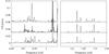 |
Fig. 5 LS power spectra of the data divided into three sub-runs; from top to bottom the independent analysis for quarters 12–17, 6–11, and 0–5 is shown. Left: StHα166 in the region of the Štefl frequencies g1 around 0.95 /¸d; some part of g2 is seen above 1 c/d. Right: the same for for HD 186567 in the region of g2. |
The most obvious features in the power spectrum are not the discrete frequencies or groups, however. Rather, it is dominated by broad bumps of power. The two strongest of these bumps were already identified by Balona et al. (2011) as the dominant feature of the spectrum. Balona et al. mention a third peak at 0.1 c/d, but in the interpretation here that peak is due to the low frequencies representing the long-term outburst and their harmonics that were removed in the pre-processing steps (see Fig. 1). It has nothing to do with the bumps at higher frequencies.
In addition to the bumps h1 at 0.9 c/d and h2 already mentioned by Balona et al. (2011), both the LS and the wavelet analysis show two further bumps at higher frequenciesh3 and h4, more prominent when the disk feeding activity is high. As the wavelet analysis makes clear, these are not groups of real frequencies. Even in the LS analysis, pre-whitening for more than one hundred frequencies within these bumps does not alter their appearance or power in any significant way. This clearly indicates aperiodic, at best short-term cyclic variations on a scale of about 0.9 c/d. The higher bumps h2 to h4 are at positions that make them likely to be a sign of the non-sinusodiality of this aperiodic variability. In particular, h1 ≈ h2/ 2 ≈ h3/ 3 ≈ h4/ 4. If h1 was due to true frequencies, h2 to h4 would be their harmonics. However, as they are not coherent frequencies, instead of being real harmonics, one may consider the bumps at higher frequencies as “group” or “statistical” harmonics (see also Paper I). Another distinctive feature of h1 and h2 is that they become broader towards lower frequencies at the time of outbursts.
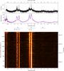 |
Fig. 6 Like Fig. 4, but for HD 186567. All data before t = 1000 are averaged into the less variable wavelet power spectrum (dashed), data after into the more variable one (solid). The label Š denotes the possible circumstellar Štefl frequency (see Sect. 4.2), seen better in the average power spectra rather than in the 2D representation. |
 |
Fig. 7 Amplitude variation with time for HD 186567. Curves were created by averaging the lowermost panel of Fig. 6 over the respective frequency regions. Top panel: A2 solid and A3 as a dashed line. Bottom panel: A1 dotted A4 dashed, and A5 as a solid line. |
3.3. HD 186567
In terms of both Be star activity and disk feeding, this star is an intermediate example between ALS 10705 and StHα166. There are no detectable outbursts in the first two years of the observations, but the star shows increasing outburst variability after t = 1000. Due to the lack of spectroscopic data one cannot tell whether the star was completely without emission before t = 1000, or rather in a disk dissipation phase, in which the circumstellar disk is still present, but no longer being fed by outbursts.
The power spectrum in both LS and wavelet analysis of HD 186567 (see Fig. 6) shows four clear frequency groups, and a number of isolated peaks. Again several correlations between the amplitude envelopes of each group exist.
The strongest features are the groups at g2 = 1.8 c/d, g3 = 2.2 c/d, g4 = 3.7 c/d, and g5 = 4 c/d, plus the peak at g1 = 0.28 c/d, numbered in the order of increasing frequency. In fact, also g1 is resolved by the LS analysis into four closely spaced frequencies, which is, however, negligible compared to the dozens of frequencies found in the other groups.The frequency value of g1 is about the difference between g4 and g5. Although g4 ≈ 2 × g2, it is different from the above mentioned statistical harmonics in the sense that here the behavior of A4 is not correlated with A2.
What is immediately seen is that the amplitude envelopes A4 and A5 are anti-correlated on the longest time scale observed, that is years. While A4 gains in power from 2009 to 2013, A5 decreases towards the end. Not obvious from Fig. 6, but well seen in Fig. 7 is that A1 follows the same trend as A5, slowly decreasing in power. A2 vs. A3 shows a similar long-term behavior, but much less pronounced: While A2 increases somewhat, A3 decreases a little (see as well Fig. 7 rather than Fig. 6).
On short time scales, there are as well correlations between the amplitude envelope curves. A2 and A3 are quite well positively correlated; certainly not perfect but clearly beyond what one would expect from random variations. A4 and A5, however, are anti-correlated, that is A4 being strong means A5 is weak and vice versa. These correlations are seen because each group has a short term variability in itself, in principle like the ones seen in ALS10705, but much faster (see Fig. 3 for comparison).
In the overall power spectra, it is also seen that there are two very broad bumps, at about h1 = 2 c/d and at about h2 = 4 c/d. A third one, h3 might be identified at about 5.5 to 6 c/d, stronger when there is disk feeding. g2 and g3 seem to be symmetrical around the center of h1, and g5 centered on h2. The behavior of the bumps is very similar to the ones in StHα166. Before t = 1000, when no signature of disk feeding is seen, they are weaker, and also a bit shifted towards higher frequencies, while when the disk is being fed after t = 1000 they are stronger and slightly shifted towards lower frequencies.
In detail, the variability properties of g2 look somewhat different from all that was described so far. Although A2 is correlated with A3, even in the wavelet analysis it is not possible to identify a single, stable frequency that would just have variable amplitude. Kurtz et al. (2015) state that the period values in a periodogram computed over observing quarters 0 to 9 are the same as the ones over quarters 10 to 17. We have repeated this exercise with quarters 0 to 5, 6 to 11, and 12 to 17, that is with a somewhat finer sampling, less susceptible to averaging. The same approach was already applied to StHα166 (see Fig. 5). The periods are indeed quite stable, although their formal differences exceed 3σ somewhat. The strongest of those frequencies, at 1.822 c/d, has an average semi-amplitude of about 1 mmag. Inspecting Fig. 6 in the region of g2 more closely, one finds the power distributed over a frequency range that is broader than the resolution of the wavelet analysis at this frequency, but still much narrower than the broad bumps. The adjacent pattern of g3 serves as a comparison how a single frequency with variable amplitude (or two stable beating frequencies) would look like.
4. Discussion
4.1. Amplitude correlations
The commonly adopted interpretation of the LS periodogram of a B type star is that of a large number of independent frequencies, which, if coming in groups, produce beating pattern with very low frequencies that show as slowly varying amplitude envelopes. This work offers nothing to actually disprove this interpretation. However, the observed correlations between the amplitude envelopes of supposedly independent frequency groups are not easily explained in such an interpretation; other explanations, in which such correlations arise more naturally, should be explored. Most typical is a negative correlation between two strong frequency groups (ALS 10705: A7/A4, HD 186567: A4/A5, possibly StHα166: A3/A4), and a strong frequency group might be accompanied by a number of weaker ones with positive correlation (ALS 10705: A7 + A10 + A13, A4 + A9, A1 + A8). However, more complicated relations are observed as well (ALS 10705: A1 vs. A7/A4). Such relations prompt the question whether there are internal processes in the star that redistribute energy between pulsation modes on short time scales back and forth. Resonant mode coupling has been described much earlier, e.g., by Dziembowski (1982), but so far the idea was applied mostly to δ Sct and RR Lyr stars, rarely to B stars.
4.2. The Štefl frequencies of StHα166
In Sect. 3.2g1 at 0.94 c/d of StHα166 is described as transient and unstable in frequency and phase. This and the presence of a more stable variation g2 at a slightly higher frequency of 1.03 c/d hallmarks it as a phenomenon often found to be associated with disk feeding, and g2 as the main stellar pulsational frequency that would be detectable by spectroscopy. Such frequencies have first been described by Štefl et al. (1998). Then they were named “transient frequencies” in reference to their non-persistent nature. For a detailed description of Štefl frequencies see Sect. 2 of Paper I.
From Fig. 5 it is clear that there is no single such frequency; rather these are fairly short-lived individual episodes of cyclic variability, which occur within a narrow frequency region of about ± 5%. Paper I, based not only on the two stars studied there, but as well re-assessing the literature, has made a strong case that this variability is directly related to the feeding of fresh stellar material into the base of the disk. Certainly the disk feeding pattern, strong in quarters 0–5 and 12–17, but weak in 6–11, agrees with this. Some part of the variability identified above as groups g3 and g4 could actually have someharmonic relation to g1. As will be shown in forthcoming papers of this series, it often is the case in Be stars that the first harmonic of a circumstellar Štefl frequency is stronger than the base frequency outside of outbursts. The alternative would be that g3 and g4 are g-modes in their own right. In the same test as shown in Fig. 5g4, just at different frequency values, is found to be stable in frequency, while g3 is not. This means that while g3 might indeed be a harmonic of g1, g4 is more likely a real g-mode pulsation.
One could argue from Fig. 6 that also in the power spectrum of HD 186567 a Štefl frequency might be present after the star began to feed the disk at about t ≈ 1000, at a frequency value of about 1.55 c/d. However, given the weak variability and the weak signature in the power spectrum, that cannot be said with certainty. We note that there is nothing like a Štefl frequency seen in the quiescent Be star ALS 10705.
4.3. Broad bumps in the power spectra
The broad bumps found in the power spectra of StHα166 and HD 186567 are well known from other Be stars. They are typically interpreted in terms of a dense population of low-order g-modes (Walker et al. 2005; Dziembowski et al. 2007; Cameron et al. 2008), though Balona (2009) has suggested a rotational or circumstellar interpretation. Here it is argued that they are indeed circumstellar, though not necessarily connected to rotation, just due to aperiodic variability residing in the circumstellar environment, that is the gaseous disk (see Paper I). The bump at very low frequencies of up to about 0.1 c/d is due to the photometric variability of the long-term outbursts of Be stars. The bump at the next higher frequency is suggested to be due to aperiodic variations on about the time scale of that frequency, while bumps at still higher frequency are (pseudo-)harmonics belonging to these aperiodic variations.
Variations on a scale of around 1 to 2 c/d are ubiquitous in Be stars. It can be g-mode pulsation,stellar rotation, or the orbital period in the inner parts of the disk. However, neither a well defined frequency nor coherence is found, and the position and strength of the bumps correlate with the strength of the disk feeding. The latter is seen in the respective middle panels of Figs. 4 and 6, where power spectra are shown, averaged for more and less strong feeding phases. The presence of a broad bump at all times in the wavelet analysis for StHα166 suggests that there are a large number of such variations present at any given time there is a disk, while the diskless ALS 10705 is free of such bumps. All these observations speak for a purely circumstellar origin, rather than a stellar, photospheric one.
Unfortunately, the Be activity status of HD 186567 during the Kepler observations is not fully known. Clear outburst were observed only after t ≈ 1000, but also before the star may well have had a circumstellar disk, either dissipating or sustained by minor outbursts only. This would have been a disk in its dissipation phase, formed during earlier outburst variability. Extended dissipation phases with no or very little outburst variability are common in Be stars (Štefl et al. 2003a; Draper et al. 2014). In any case, in HD 186567 there was a growing number of outbursts after t = 1000, and the strength of the bumps h1 and h2 increased, while the previously barely detectable h3 became much clearer as outburst variability began.
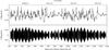 |
Fig. 8 Combined variation of the g2 group of StHα166, reconstructed with the frequencies in Table 2 (bottom panel) compared to the long-term outburst variability of the star (upper panel, see also middle panel of Fig. 1). |
4.4. Outbursts and pulsation of StHα166
A detailed analysis of StHα166 concerning the relation between the outbursts and the pulsational behavior is out of the scope of this work. However, already in the analysis here a relation akin to μ Cen (see Rivinius et al. 1998) between the combined amplitude of g2 and the outbursts is seen (see Fig. 8), i.e., amplitude maxima of g2 co-incide with outbursts. In the first 120 iterations of the LS analysis a total of nine frequencies were found that belong to g2 (Table 2). Independent of the interpretation as real frequencies or just a mathematical representation of the overall evolution of a single, true frequency, the co-added variations of those nine frequencies describe the behavior of A2, just as the co-added low frequencies describe the secular behavior. The amplitude reconstruction is compared to the long-term outburst evolution in Fig. 8. Both the long-term evolution of the reconstructed amplitude, maxima at t ≈ 350 and t ≈ 1150, as well as the short-term structure with intermediate maxima every ≈50 days, and further sub-maxima even more often, agree well with the temporal evolution of the outbursts of StHα166. The nine periods of g2 (Table 2) can be grouped again in three sub-groups seperated by about 0.02 c/d, which is also the frequency value where the by far highest power is found in the LS-analysis of the long-term tends (≈0.02 c/d, or 50 days as mentioned above). This may be the same type of behavior as seen in η Cen (see Paper I), where the frequency difference of two close stellar frequencies is seen with high amplitude not as a beating phenomenon, but as a frequency in its own right with much higher amplitude than the two original frequencies.
4.5. The g1 and g2 groups of HD 186567
The frequency value of g1 = 0.28 c/d of this not very variable Be star of late B subtype is about the difference of two much higher frequencies, g4 and g5. A rotation period of about 3.5 d would be unbelievably long for a Be star, which are thought to be rotating close to the critical limit. If g1 is not a true pulsation mode, in which case it would have to be a retrograde ’g-mode, see Sect. 4.6, it is a combination frequency of g4 and g5. Such frequencies have been found in Be stars (e.g., in η Cen, PaperI, or in ω CMa, Sect. 4.1 of Štefl et al. 2003a), but hitherto known examples are typically much longer, tens of days. Also, in those stars the difference frequencies seem linked to disk feeding, for which no sign was found in HD 186567, except during a few short episodes in the second half of the observational time base.
The frequency group g2 shows a rather puzzling appearance in the wavelet analysis. Dividing the data into three sub-sets and analyzing them individually by LS reveals an ensemble of frequencies that is possibly not entirely identical to each other in frequency and certainly quite variable in amplitude, but far more stable than one would expect from a mere time scale, as are the Štefl frequencies of StHα166 (both shown in Fig. 5). Also that g2 in HD 186567 has a rather sharp border in frequency space (see Fig. 6) is not really what one would expect from aperiodic variablity of a given time scale.
One possibility is certainly that the sub-frequencies of g2 as apparent in Fig. 5 are real, and the pattern seen in the wavelet analysis is the result of a beat pattern in which the variable amplitudes of the individual sub-frequencies destroy the coherent appearance.
To investigate this possibility a total of 40 B stars from the CoRoT database, flagged as β Cep or SPB stars by either Degroote et al. (2009) or Sarro et al. (2013), were analyzed in the same way (the full results will be presented in a future work of this series on the Be stars found in the CoRoT database). Two β Cep stars, CoRoT ID101024938 and CoRoT ID106113525 showed unresolved strips of multi-mode pulsational power like HD 186567. However, their appearance is far more regular, that is power minima and maxima follow a clearly ordered and periodic pattern both in temporal sequence and in frequency position.
Therefore, since the frequencies were found to be stable in Fig. 5, the distinct appearance in Fig. 6 must be due to unstable amplitudes. Looking for possible explanations, the wavelet analysis may also be compared to what Belkacem et al. (2009) have suggested to be the signature of stochastic oscillations forthe β Cepheid V1449 Aql (see their Fig. 2). Stochastically excited oscillations are theoretically predicted to occur across the B star spectral range (see, e.g., Shiode et al. 2013; Mathis et al. 2014; Lee et al. 2014). Judging from Fig. 6of Shiode et al., however, the observed amplitude of 1 mmag seems to be about 1 order of magnitude higher than what is expected. Given the fast rotation of a Be star, the observed frequency being twice as high as the highest one in the co-rotating frame of the star is less of a concern, as will be seen below. For the case of V1449 Aql this explanation is not unequivocally accepted; Aerts et al. (2011) have suggested non-linear resonance arising from the interaction of a large number of other modes, while Degroote (2013) proposes that the dominant radial mode of V1449 Aql produces this signature through chaotic behavior. In any case, the similarity of the signature in the wavelet analysis remains striking, and the positive amplitude correlation between A2 and A3 could well be a clue towards the model of Aerts et al.
4.6. Rotation and frequencies in Be stars
For non-radial pulsations in a rotating star, the observed period is not the one in the co-rotating frame of the star. While in most stars the rotation rates are low enough for the difference to be of only minor importance, this is not so for Be stars. In general, the observed and co-rotating frequencies fobs and fcorot are related to each other via  (2)where Ω is the rotation frequency of the star and m is the azimuthal number of the non-radial pulsation. By convention negative m denote a pulsation that is propagating prograde in the co-rotating frame of the star. Obviously, a prograde mode cannot be observed at frequencies lower than Ω. For retrograde modes the relation between observed and co-rotating frequency can be less obvious. A mathematically negative fobs means the variation appears prograde to the observer, but | fobs | > Ω is well possible. For rapid rotators, as Be stars are, all the above means that the simple classification as p- or g-mode pulsator, based solely on the value of fobs being lower or higher than some division line (often 4 c/d is chosen as delimiter), becomes invalid. For example, a perfectly ordinary g-mode, say fcorot =1 c/d, with ℓ = 2,m = −2, on a perfectly ordinary Be star, say rotating at 1.5 c/d, would be observed at 4 c/d, and hence be classified as a p-mode. For this reason, stars like ALS 10705 or HD 186567 might not actually be hybrid pulsators, as they were classified, but pure g-mode pulsators.
Rotation also poses a certain challenge to the suggestion by Kurtz et al. (2015) that combination frequencies are responsible for non-linear appearance of some light-curves. Combination frequencies are observed frequencies that relate to other observed frequencies via  (3)However, in order to interact in such a way as to produce non-linear effects, as suggested by Kurtz et al., the interaction must be physical in the object, as otherwise the variations would just superimpose linearly, and not produce detectable power in the periodogram at the combination frequency. In other words, the simple combination with integer numbers n must exist also in the co-rotating frame of the star. This only works if the sum of all terms nimi (m again the azimuthal number), becomes zero, which severely limits the potential of combination frequencies to explain frequency groups, at least for rapid rotators.
Frequencies belonging to the g2 group of StHα166, found in the first 120 steps of the LS analysis.
Indeed, while for the slowly rotating γ Dor star KIC 8113425 Kurtz et al. only need four genuine frequencies to explain 39 further frequencies as combinations, the ratio is the opposite for the Be star HD 186567: for 15 frequencies they regard as genuine (all of which are from the g2 group, which is discussed in some detail above), they only find four combination frequencies present in the periodogram.
5. Conclusions
Among the stars observed by the Kepler spacecraft, three have been identified as Be stars in the literature. By good fortune, these three provide good examples covering the full range of Be star behavior: ALS 10705 is inactive without disk; HD 186567 exhibits increasing disk feeding by outbursts, possibly with a decaying previous disk; and StHα166 is a fully active Be star showing strong, ongoing outbursts. The commonalities and differences found are suggested to be a general scheme for the photometric behavior of Be stars as follows:
The stellar power spectrum of a Be star in an inactive phase.
Comparing the results for the Be star ALS 10705, observed in quiescence, to the literature, nothing is found in the LS analysis that is different in principle from the appearance of non-emission B stars. That Be stars have a tendency to be classified as hybrid pulsators, even when well outside the β Cep instability strip, is possibly a consequence of their rapid rotation, rather than due to the true presence of high-order p-modes. In the co-rotating frame of the star all photospheric periods can well reside in the low frequency g-mode regime, depending on their mode properties ℓ and in particular m.
There are correlations between the amplitude variability of individual modes (or mode groups, if understood as a beating phenomenon) which need an explanation. In case of single modes that might be resonant mode-coupling in the stellar interior, in the case of mode groups a mechanism would have to be found; none has to our knowledge been proposed. Similar correlations for SPB and β Cep stars are not known, but that could rather be due to the usage of LS dominating the literature instead of wavelet analysis for such stars.
Any LS analysis over the entire time span of observations should, therefore, only be the first step in analyzing Be star variability; it must be followed by time-resolved ways to analyze the variation, such as wavelet, or LS with a running box-filter in the time domain. In this work the wavelet approach was adopted for its robustness (see discussion in Foster 1996) and the frequency resolution being a function of frequency of the form of R = Δf/f = const., which is well suited for the problem of tracking the behavior of frequency groups over a wide range of frequencies.
A variable amplitude is also seen in the g2 group of HD 186567, without being resolved into beatings even in the full Kepler run. From an observational point of view, amplitude variability on time scales longer than the time base of typical observing runs is the norm in Be stars, not the exception, regardless of whether one interpretes this variability as intrinsic or as due to unresolved beating.
The circumstellar power spectrum of a Be star in an active phase, but without outbursts.
For the first about 1000 days of the Kepler observations, HD 186567 did not show any sign of out bursts, which began around t = 1000 and continued until the end of the observation. However, already before the outbursts started, its power spectrum differed from that of the fully inactive ALS 10705 by the additional presence of broad bumps in the power spectrum. Above, these were associated with the presence of a disk in the circumstellar environment, and as HD 186567 turned to disk feeding by outbursts they increased in strength and moved towards longer frequencies. The same behavior of the bumps can be seen in StHα166 comparing the times of strong and weak disk feeding.
In summary, it seems that the bumps are associated with the plain presence of a disk, and are stronger when the disk is actively fed. In terms of the viscous decretion disk model, in which the evolution of the disk after its formation is fully governed by viscous processes (see Rivinius et al. 2013, for a review), this would mean that the bump strength and position depends on the density and possibly density slope of the innermost parts of the disk.
The circumstellar power spectrum of a Be star in an active phase with outbursts.
When a Be star is having clear outbursts, it shows the broad bumps as discussed above, but stronger, in addition to the purely stellar variations. Whether the bumps are associated to the outbursts themselves, that is the ejection of matter, or the subsequent re-accretion of (part of) the ejected matter cannot be said with the data at hand, both remains possible. It should be noted that such re-accretion is an unavoidable feature of the viscous processes governing the disk.
Whether some part of the purely stellar variations are attenuated, as seems to be the case in some stars observed by CoRoT (e.g., Huat et al. 2009), can also not be said with the Kepler data alone. In any case the frequency spectrum, in terms of well defined groups, seems poorly populated compared to ALS 10705 and HD 186567. The literature shows that the possibility of attenuation in strong outburst phases exists, see also Štefl et al. (2003b) for spectroscopically equivalent behavior of ω CMa, and the absence of the spectroscopically found frequencies of μ Cen in BRITE data (see Paper I).
In addition to the above, the power spectrum increases at a characteristic frequency range, typically in the range 1–2 c/d at a value some 10% lower than that of a strong stellar pulsation mode. This latter, stellar pulsation, could be spectroscopically identified as ℓ = m = 2g-modes in most stars (Rivinius et al. 2003).
For the transient frequencies in outbursts the term Štefl frequencies is used, following Paper I. Štefl frequencies are immediately related to outbursts, that is the transfer of matter (and angular momentum) from the star into the circumstellar disk. Any individual event is short lived, and subsequent events do not repeat at the same frequency or with any phase coherency. However, as a phenomenon they are well defined and have been identified in a number of stars (see discussion in Paper I).
In further works of this series, the above findings will be tested against the databases collected by the MOST (Walker et al. 2003), CoRoT (Auvergne et al. 2009), and BRITE Constellation satellites (Weiss et al. 2014), and possibly the Kepler K2 mission. Data available from MOST, CoRoT, and K2 databases are of similar precision as the Kepler data used here, but provide shorter time bases for analysis. However, the Be stars in these databases are much more numerous, offering the opportunity to get a statistical hold on the above described phenomena. BRITE data, in turn, are less precise, and the typical campaign lengths are similar to MOST, CoRoT, or K2. However, BRITE focuses on stars with V< 5 mag, meaning it observes targets for which potentially a lot of archival data exist and often considerably detailed analysis works have been published. BRITE has the potential to link the variability types found in the Kepler data to other observables from a wide range of techniques, and will allow to make the connection to the actual physical processes much more robust than is possible with Kepler, MOST, K2, or CoRoT data alone. Paper I of this series, presenting the analysis of the BRITE observations of μ Cen and η Cen, serves as an example for the power of such an approach.
v1.32, available at http://www.astro.princeton.edu/~jhartman/vartools.html
Acknowledgments
The authors dedicate this work to Stanislav (Stan) Štefl (1955–2014) in whose honor the Štefl frequencies are named. A. C. C. acknowledges support from CNPq (grant 307594/2015-7) and FAPESP (grant 2015/17967-7). The authors are very grateful to an anonymous referee for comments serving to clarify the results. This paper includes data collected by the Kepler mission. Funding for the Kepler mission is provided by the NASA Science Mission directorate. Some of the data presented in this paper were obtained from the Mikulski Archive for Space Telescopes (MAST). STScI is operated by the Association of Universities for Research in Astronomy, Inc., under NASA contract NAS5-26555. Support for MAST for non-HST data is provided by the NASA Office of Space Science via grant NNX09AF08G and by other grants and contracts. This research used the facilities of the Canadian Astronomy Data Centre operated by the National Research Council of Canada with the support of the Canadian Space Agency. Partly based on observations obtained at the Canada-France-Hawaii Telescope (CFHT) which is operated by the National Research Council of Canada, the Institut National des Sciences de l’Univers of the Centre National de la Recherche Scientique of France, and the University of Hawaii. This research has made use of NASA’s Astrophysics Data System Service, as well as of the SIMBAD database, operated at CDS, Strasbourg, France.
References
- Aerts, C., Briquet, M., Degroote, P., Thoul, A., & van Hoolst, T. 2011, A&A, 534, A98 [NASA ADS] [CrossRef] [EDP Sciences] [Google Scholar]
- Auvergne, M., Bodin, P., Boisnard, L., et al. 2009, A&A, 506, 411 [NASA ADS] [CrossRef] [EDP Sciences] [Google Scholar]
- Baade, D., Rivinius, T., Pigulski, A., et al. 2016, A&A, 588, A56, (Paper I) [NASA ADS] [CrossRef] [EDP Sciences] [Google Scholar]
- Balona, L. A. 2009, in Stellar pulsation: Challenges for theory and observation, eds. J. A. Guzik, & P. A. Bradley, ATP Conf. Ser., 1170, 339 [Google Scholar]
- Balona, L. A., Baran, A. S., Daszyńska-Daszkiewicz, J., & De Cat, P. D. 2015, MNRAS, 451, 1445 [NASA ADS] [CrossRef] [Google Scholar]
- Balona, L. A., Pigulski, A., Cat, P. D., et al. 2011, MNRAS, 413, 2403 [NASA ADS] [CrossRef] [Google Scholar]
- Belkacem, K., Samadi, R., Goupil, M.-J., et al. 2009, Science, 324, 1540 [NASA ADS] [CrossRef] [Google Scholar]
- Cameron, C., Saio, H., Kuschnig, R., et al. 2008, ApJ, 685, 489 [NASA ADS] [CrossRef] [Google Scholar]
- Degroote, P. 2013, MNRAS, 431, 2554 [NASA ADS] [CrossRef] [Google Scholar]
- Degroote, P., Aerts, C., Ollivier, M., et al. 2009, A&A, 506, 471 [NASA ADS] [CrossRef] [EDP Sciences] [Google Scholar]
- Downes, R. A., & Keyes, C. D. 1988, AJ, 96, 777 [NASA ADS] [CrossRef] [Google Scholar]
- Draper, Z. H., Wisniewski, J. P., Bjorkman, K. S., et al. 2014, ApJ, 786, 120 [NASA ADS] [CrossRef] [Google Scholar]
- Dziembowski, W. A. 1982, Acta Astron., 32, 147 [NASA ADS] [Google Scholar]
- Dziembowski, W. A., Daszyńska-Daszkiewicz, J., & Pamyatnykh, A. A. 2007, Commun. Asteroseismol., 150, 213 [NASA ADS] [CrossRef] [Google Scholar]
- Foster, G. 1996, AJ, 112, 1709 [NASA ADS] [CrossRef] [Google Scholar]
- Hartman, J. D., Gaudi, B. S., Holman, M. J., et al. 2008, ApJ, 675, 1254 [NASA ADS] [CrossRef] [Google Scholar]
- Haubois, X., Carciofi, A. C., Rivinius, T., Okazaki, A. T., & Bjorkman, J. E. 2012, ApJ, 756, 156 [NASA ADS] [CrossRef] [Google Scholar]
- Huat, A.-L., Hubert, A.-M., Baudin, F., et al. 2009, A&A, 506, 95 [NASA ADS] [CrossRef] [EDP Sciences] [Google Scholar]
- Huber, D., Silva Aguirre, V., Matthews, J. M., et al. 2014, ApJS, 211, 2 [NASA ADS] [CrossRef] [Google Scholar]
- Koch, D. G., Borucki, W. J., Basri, G., et al. 2010, ApJ, 713, L79 [NASA ADS] [CrossRef] [Google Scholar]
- Kohoutek, L., & Wehmeyer, R. 1999, A&AS, 134, 255 [NASA ADS] [CrossRef] [EDP Sciences] [Google Scholar]
- Kurtz, D. W., Shibahashi, H., Murphy, S. J., Bedding, T. R., & Bowman, D. M. 2015, MNRAS, 450, 3015 [NASA ADS] [CrossRef] [Google Scholar]
- Lee, U., Neiner, C., & Mathis, S. 2014, MNRAS, 443, 1515 [NASA ADS] [CrossRef] [Google Scholar]
- Mathis, S., Neiner, C., & Tran Minh, N. 2014, A&A, 565, A47 [NASA ADS] [CrossRef] [EDP Sciences] [Google Scholar]
- McNamara, B. J., Jackiewicz, J., & McKeever, J. 2012, AJ, 143, 101 [NASA ADS] [CrossRef] [Google Scholar]
- Nielsen, M. B., Gizon, L., Schunker, H., & Karoff, C. 2013, A&A, 557, L10 [NASA ADS] [CrossRef] [EDP Sciences] [Google Scholar]
- Pigulski, A., Pojmański, G., Pilecki, B., & Szczygieł, D. M. 2009, Acta Astron., 59, 33 [NASA ADS] [Google Scholar]
- Press, W. H., Teukolsky, S. A., Vetterling, W. T., & Flannery, B. P. 1992, Numerical recipes in C. The art of scientific computing, 2nd edn. (Cambridge University Press) [Google Scholar]
- Reinhold, T., Reiners, A., & Basri, G. 2013, A&A, 560, A4 [NASA ADS] [CrossRef] [EDP Sciences] [Google Scholar]
- Rivinius, T., Baade, D., Štefl, S., et al. 1998, in Cyclical Variability in Stellar Winds, Proc. ESO Workshop, eds. L. Kaper, & A. W. Fullerton, 207 [Google Scholar]
- Rivinius, T., Baade, D., & Štefl, S. 2003, A&A, 411, 229 [NASA ADS] [CrossRef] [EDP Sciences] [Google Scholar]
- Rivinius, T., Carciofi, A. C., & Martayan, C. 2013, A&ARv, 21, 69 [Google Scholar]
- Sarro, L. M., Debosscher, J., Neiner, C., et al. 2013, A&A, 550, A120 [NASA ADS] [CrossRef] [EDP Sciences] [Google Scholar]
- Shiode, J. H., Quataert, E., Cantiello, M., & Bildsten, L. 2013, MNRAS, 430, 1736 [NASA ADS] [CrossRef] [Google Scholar]
- Štefl, S., Baade, D., Rivinius, T., et al. 1998, in A Half Century of Stellar Pulsation Interpretation, eds. P. A. Bradley, & J. A. Guzik, ASP Conf. Ser., 135, 348 [Google Scholar]
- Štefl, S., Baade, D., Rivinius, T., et al. 2003a, A&A, 402, 253 [NASA ADS] [CrossRef] [EDP Sciences] [Google Scholar]
- Štefl, S., Baade, D., Rivinius, T., et al. 2003b, A&A, 411, 167 [NASA ADS] [CrossRef] [EDP Sciences] [Google Scholar]
- Stephenson, C. B. 1986, ApJ, 300, 779 [NASA ADS] [CrossRef] [Google Scholar]
- Walker, G., Matthews, J., Kuschnig, R., et al. 2003, PASP, 115, 1023 [NASA ADS] [CrossRef] [Google Scholar]
- Walker, G. A. H., Kuschnig, R., Matthews, J. M., et al. 2005, ApJ, 635, L77 [NASA ADS] [CrossRef] [Google Scholar]
- Weiss, W. W., Rucinski, S. M., Moffat, A. F. J., et al. 2014, PASP, 126, 573 [NASA ADS] [CrossRef] [Google Scholar]
- Zechmeister, M., & Kürster, M. 2009, A&A, 496, 577 [NASA ADS] [CrossRef] [EDP Sciences] [Google Scholar]
All Tables
Comparison of frequency groups found in the wavelet vs. the dominant frequency of each group found in the LS analysis of ALS 10705.
Frequencies belonging to the g2 group of StHα166, found in the first 120 steps of the LS analysis.
All Figures
|
Fig. 1 Long-term part of the variability removed by high-pass filtering in black, original data gray in background. For this plot, linear trends have been removed beforehand. Shown are, from top to bottom, ALS 10705, StHα166, and HD 186567. There is a difference in vertical scale, and hence amplitude of the variations. |
| In the text | |
|
Fig. 2 Time series analysis of ALS 10705. From top to bottom the LS periodogram, the time averaged result of the wavelet analysis, both shown in logarithmic scale, and the full 2D result of the wavelet analysis, where the intensity is displayed in logarithmic scale, too. The frequency groups discussed in the text are identified above the lowermost panel. |
| In the text | |
|
Fig. 3 Amplitude variation with time for g1, g8, g4 and g7 (top to bottom) of ALS 10705. The individual points were computed by co-adding the fits to all frequencies found by LS belonging to each group, and then the absolute value was plotted. The upper envelope of each group, therefore, represents the amplitude variations seen in the lower panel of Fig. 2 and illustrates the various correlations described in the text. |
| In the text | |
|
Fig. 4 Like Fig. 2, but for StHα166. In the middle panel, instead of the overall wavelet power spectrum, the average power spectrum during more variable phases (t< 700 and 900 <t< 1500) is shown in as a solid line, during less variable (700 <t< 900 and t> 1500) as a dashed one. The label Š denotes the circumstellar Štefl frequencies (see Sect. 4.2). |
| In the text | |
|
Fig. 5 LS power spectra of the data divided into three sub-runs; from top to bottom the independent analysis for quarters 12–17, 6–11, and 0–5 is shown. Left: StHα166 in the region of the Štefl frequencies g1 around 0.95 /¸d; some part of g2 is seen above 1 c/d. Right: the same for for HD 186567 in the region of g2. |
| In the text | |
|
Fig. 6 Like Fig. 4, but for HD 186567. All data before t = 1000 are averaged into the less variable wavelet power spectrum (dashed), data after into the more variable one (solid). The label Š denotes the possible circumstellar Štefl frequency (see Sect. 4.2), seen better in the average power spectra rather than in the 2D representation. |
| In the text | |
|
Fig. 7 Amplitude variation with time for HD 186567. Curves were created by averaging the lowermost panel of Fig. 6 over the respective frequency regions. Top panel: A2 solid and A3 as a dashed line. Bottom panel: A1 dotted A4 dashed, and A5 as a solid line. |
| In the text | |
|
Fig. 8 Combined variation of the g2 group of StHα166, reconstructed with the frequencies in Table 2 (bottom panel) compared to the long-term outburst variability of the star (upper panel, see also middle panel of Fig. 1). |
| In the text | |
Current usage metrics show cumulative count of Article Views (full-text article views including HTML views, PDF and ePub downloads, according to the available data) and Abstracts Views on Vision4Press platform.
Data correspond to usage on the plateform after 2015. The current usage metrics is available 48-96 hours after online publication and is updated daily on week days.
Initial download of the metrics may take a while.