© ESO, 2016

1. Introduction

The δ Scuti stars are a class of pulsating stars falling in the Hertzsprung-Russel diagram where the main sequence overlaps the lower extension of the Cepheid instability strip (Breger 2000; Aerts et al. 2010). They are in the core hydrogen-burning or shell-hydrogen-burning stage (Aerts et al. 2010), with masses from 1.5 M_⊙ to 2.5 M_⊙ (Aerts et al. 2010) and pulsation periods from 0.5 to 6 hours (Breger 2000). Their pulsations are driven by the κ mechanism (Baker & Kippenhahn 1962, 1965; Zhevakin 1963; Li & Stix 1994) in the second partial ionization zone of helium. Some of δ Scuti stars show multi-period pulsations, such as 4 Cvn (Breger et al. 1999), FG Vir (Breger et al. 2005), and HD 50870 (Mantegazza et al. 2012), and are therefore good candidates for asteroseismological studies.

HD 50844 was discovered to be a δ Scuti variable star by Poretti et al. (2005) during their preparatory work for the CoRoT mission. The basic physical parameters of HD 50844 were also obtained by Poretti et al. (2005) from Str$\begin{array}{c}{\mathrm{¨}}_{}\\ \mathrm{o}\end{array}$mgren photometry. They are listed as follows: T_eff = 7500 ± 200 K, log g = 3.6 ± 0.2, and [Fe/H] = −0.4± 0.2. High-resolution spectroscopic observations obtained with the FEROS instrument mounted on the 2.2-m ESO/MPI telescope at La Silla resulted in the value of υsini = 58 ± 2 km s^-1 and the inclination angle i = 82 ± 4 deg (Poretti et al. 2009).

HD 50844 was observed from 2 February 2007 to 31 March 2007 (Δt = 57.61 d) by CoRoT during the initial run (IR01). Detailed frequency analysis of the observed timeseries by Poretti et al. (2009) revealed very dense frequency signals in the range of 0–30 d^-1. In particular, they identified the frequency 6.92 d^-1 with the largest amplitude as the fundamental radial mode by combining spectroscopic and photometric data. Meanwhile, very high-degree oscillation modes (up to l = 14) were identified by Poretti et al. (2009) with the software FAMIAS (Zima 2008) to fit the line profile variations (Mantegazza 2000). Based on an independent analysis, Balona (2014) arrived at the conclusion that a normal mode density may exist for the CoRoT timeseries of HD 50844. He extracts a total of 59 significant oscillation modes from the CoRoT timeseries.

Asteroseismology is a powerful tool to investigate the internal structure of pulsating stars that show rich pulsation modes in observations, such as 44 Tau (Civelek et al. 2001; Kırbıyık et al. 2003; Garrido et al. 2007; Lenz et al. 2008, 2010) and α Oph (Zhao et al. 2009; Deupree et al. 2012). Mode identifications are very important for asteroseismic studies of δ Scuti stars. Any eigenmode of stellar nonradial oscillations can be characterized by its radial order k, spherical harmonic degree l, and azimuthal number m (Christensen-Dalsgaard 2003). For δ Scuti stars, there are usually only a few observed modes to be identified, such as FG Vir (Daszy$\begin{array}{c}{\mathrm{´}}_{}\\ \mathrm{n}\end{array}$ska-Daszkiewicz et al. 2005; Zima et al. 2006) and 4 Cvn (Castanheira et al. 2008; Schmid et al. 2014). Observed frequencies of a pulsating star could be compared with the results of theoretical models only if their values (l, m) have been determined in advance.

For a rotating star, a non-radial oscillation mode will split into 2l + 1 different components. According to the asymptotic theory of stellar oscillations, the 2l + 1 components of one mode of (k, l) are separated by almost the same spacing for a slowly rotating star. In our work, we try to identify the observed frequencies obtained by Balona (2014), based on the rotational splitting law of g-mode. Then we compute a grid of theoretical models to examine whether the computed stellar models can provide a reasonable fit to the observed frequencies. In Sect. 2, we analyse the rotational splitting of the observational data. In Sect. 3, we describe our stellar models, including input physics in Sect. 3.1 and details of the grid of stellar models in Sect. 3.2. Our fitting results are analysed in Sect. 4. Finally, we summarize our results in Sect. 5.

2. Analysis of rotational splitting

As already pointed out by Poretti et al. (2005), HD 50844 is in the post-main-sequence evolution stage with a contracting helium core and an expanding envelope. The steep gradient of chemical abundance in the hydrogen-burning shell will result in a large Brunt-V$\begin{array}{c}{\mathrm{¨}}_{}\\ \mathrm{a}\end{array}$is$\begin{array}{c}{\mathrm{¨}}_{}\\ \mathrm{a}\end{array}$l$\begin{array}{c}{\mathrm{¨}}_{}\\ \mathrm{a}\end{array}$ frequency N there. As a result, there are two propagation zones inside the star: one for g modes in the helium core and the other for p modes in the stellar envelope. As already pointed out by Poretti et al. (2009), most of the observed pulsation modes for HD 50844 should be gravity and mixed modes. The mixed modes are dominated by two characteristics. They have pronounced g-mode character in the helium core and p-mode character in the stellar envelope. In our work, we pay more attention to those modes that have frequencies near or higher than that of the fundamental radial mode (ν> 75μ Hz). We list 40 frequencies obtained by Balona (2014) in Table 1. Errors of the observed frequencies obtained by Balona (2014) are too small, i.e., less than 0.0015 μHz. These are not listed in Table 1.

The approximate expression for rotational splitting (δν_k,l) and rotational period (P_rot) for g-mode was derived by Dziembowski & Goode (1992) as 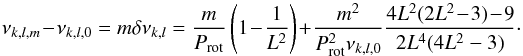${\mathit{\nu }}_{\mathit{k,l,m}}\mathrm{-}{\mathit{\nu }}_{\mathit{k,l,}\mathrm{0}}\mathrm{=}\mathit{m\delta }{\mathit{\nu }}_{\mathit{k,l}}\mathrm{=}\frac{\mathit{m}}{{\mathit{P}}_{\mathrm{rot}}}\left(\mathrm{1}\mathrm{-}\frac{\mathrm{1}}{{\mathit{L}}^{\mathrm{2}}}\right)\mathrm{+}\frac{{\mathit{m}}^{\mathrm{2}}}{{\mathit{P}}_{\mathrm{rot}}^{\mathrm{2}}{\mathit{\nu }}_{\mathit{k,l,}\mathrm{0}}}\frac{\mathrm{4}{\mathit{L}}^{\mathrm{2}}\mathrm{(}\mathrm{2}{\mathit{L}}^{\mathrm{2}}\mathrm{-}\mathrm{3}\mathrm{)}\mathrm{-}\mathrm{9}}{\mathrm{2}{\mathit{L}}^{\mathrm{4}}\mathrm{(}\mathrm{4}{\mathit{L}}^{\mathrm{2}}\mathrm{-}\mathrm{3}\mathrm{)}}\mathrm{·}$(1)In Eq. (1), L² = l(l + 1), and m ranges form −l to l, resulting in 2l + 1 different values. Considering υsini = 58 ± 2 km s^-1 of HD 50844 (Poretti et al. 2009), the second term on the right-hand side of Eq. (1) is very small (e.g., less than 1.6% of the value of the first term for $\frac{\mathrm{1}}{{\mathit{P}}_{\mathrm{rot}}}$ = 5 μHz and ν_k,l,0 = 100 μHz). Therefore, only the first-order effect is considered in our work.

According to Eq. (1), modes with l = 1 constitute a triplet. Modes with l = 2 constitute a quintuplet, and modes with l = 3 constitute a septuplet. Meanwhile, the rotational splitting of l = 1 modes and those of l = 2 modes and l = 3 modes are in some certain proportion, i.e., δν_{k,l = 1}:δν_{k,l = 2}:$\mathit{\delta }{\mathit{\nu }}_{\mathit{k,l}\mathrm{=}\mathrm{3}}\mathrm{=}\frac{\mathrm{3}}{\mathrm{5}}$:1:$\frac{\mathrm{11}}{\mathrm{10}}$ (Winget et al. 1991). Furthermore, the values of rotational splitting are very close for modes with l ≥ 3, e.g., the differences of rotational splittings between modes with l = 4 and those with l = 3 are about $\frac{\mathrm{0.033}}{{\mathit{P}}_{\mathrm{rot}}}$. If one complete nontuplet is identified, these modes can be identified as modes with l = 4. But beyond that, it is difficult to distinguish multiplets of l = 4 and higher values from those of l = 3. High spherical harmonic degree modes are detected in spectroscopy of several δ Scuti stars, such as HD 101158 (Mantegazza 1997) and BV Cir (Mantegazza et al. 2001). There is no complete nontuplet to be identified for HD 50844, thus modes with l ≥ 4 are not considered in our work.

Based on the above considerations, there are two properties of the frequency splitting because of rotation. Firstly, the 2l + 1 splitting frequencies of one mode are separated by a nearly equal split. Secondly, rotational splittings derived from modes with different spherical harmonic degree l are in specific proportion. Frequency differences ranging from 1 μHz to 20 μHz are searched for the observed frequencies. Possible multiplets due to rotational splitting are listed in Table 2.

In Table 2, we can see that (f₂₁, f₂₂, f₂₃) and (f₂₇, f₂₉, f₃₃) constitute two multiplets with an averaged frequency difference δν₁ of 2.434 μHz, and (f₉, f₁₁, f₁₄) constitute another multiplet with an averaged frequency difference δν₂ of 8.017 μHz. It is worth noting that the ratio of δν₁ and δν₂/2 is 0.607, which agrees well with the property of g-mode rotational splitting (Winget et al. 1991). Therefore, (f₂₁, f₂₂, f₂₃) and (f₂₇, f₂₉, f₃₃) are identified as two complete triplets, which are denoted as Multiplet 1 and Multiplet 2 in Table 2. Poretti et al. (2009) performed mode identifications with the FAMIAS method. They identified f₂₁ as (l = 3, m = 3), f₂₃ as (l = 3, m = 2), and f₃₃ as (l = 3, m = 1). Besides, (f₉, f₁₁, f₁₄) is identified as modes with l = 2 on the basis of the ratio of δν₁ and δν₂/2. Values of azimuthal number m for f₉, f₁₁, and f₁₄ are then identified as being m = (−2,0, + 2). Poretti et al. (2009) identified f₉ as a low l mode. Moreover, the value of δν_{k,l = 1} is estimated to be 2.434 μHz, δν_{k,l = 2} to be 4.009 μHz, and δν_{k,l = 3} to be 4.462 μHz.

Frequencies of f₂₄ and f₂₅ may constitute Multiplet 3 with a frequency difference of 2.431 μHz, which is approximate to δν_{k,l = 1}. We may identify their spherical harmonic degree as l = 1. When identifying their azimuthal number m, there are two possibilities, i.e., corresponding to modes of m = (−1,0) or m = (0, + 1). Poretti et al. (2009) identified f₂₄ as (l = 5, m = 3).

Frequencies of f₁ and f₅ may constitute Multiplet 5 with a frequency difference of 8.072 μHz, which is about twice that of δν_{k,l = 2}. We can identify their spherical harmonic degree as l = 2. When identifying their azimuthal number m, there are three possibilities, i.e., corresponding to modes of m = (−2,0), m = (0, + 2), or m = (−1, +1).

Besides, the frequency difference between f₁₅ and f₁₈ is 3.939 μHz and the frequency difference between f₃₅ and f₃₆ is 3.983 μHz. Both of them are approximate to δν_{k,l = 2}. We may identify their spherical harmonic degree as l = 2. There are four possible identifications for their azimuthal number m, i.e., corresponding to modes of m = (−2, −1), m = (−1,0), m = (0, +1), or m = (+1, 2). Poretti et al. (2009) identify f₁₅ as (l = 8, m = 5) and f₃₅ as (l = 12, m = 10).

In Table 2 we can see that (f₂, f₇), (f₁₂, f₂₀), and (f₃₈, f₃₉) may constitute three independent multiplets. The frequency difference between f₂ and f₇ is 12.228 μHz. The frequency difference between f₁₂ and f₂₀ is 11.825 μHz, and the frequency difference between f₃₈ and f₃₉ is 11.890 μHz. All of these frequency differences are about three times that of δν_{k,l = 2}. We may identify their spherical harmonic degree as l = 2. When identifying their azimuthal number m, there are two possibilities, i.e., corresponding to modes of m = (−2, + 1) or m = (−1, + 2). Poretti et al. (2009) identified f₁₂ as (l = 3, m = 1), and f₃₉ as (l = 14, m = 12).

Three frequencies of f₃, f₆, and f₈ may constitute Multiplet 11. The frequency difference 8.985 μHz between f₃ and f₆ is about twice that of δν_{k,l = 3}, and the frequency difference 13.412 μHz between f₆ and f₈ is about three times that of δν_{k,l = 3}. Their spherical harmonic degree l can be determined as being l = 3. There are two possible identifications for their azimuthal number m, i.e., corresponding to modes of m = (−3,−1, +2) or m = (−2,0, + 3).

Another three frequencies of f₁₀, f₁₇, and f₁₉ may constitute Multiplet 12. The frequency difference 17.253 μHz between f₁₀ and f₁₇ is about four times that of δν_{k,l = 3}, and the frequency difference 4.302 μHz between f₁₇ and f₁₉ is approximate to δν_{k,l = 3}. We may identify their spherical harmonic degree as l = 3. When identifying their azimuthal number m, there are two possibilities, i.e., corresponding to modes of m = (−3, + 1, + 2) or m = (−2, + 2, + 3). Poretti et al. (2009) identify f₁₀ as (l = 5, m = 0), and f₁₇ as (l = 11, m = 7).

Four frequencies of f₂₆, f₂₈, f₃₄, and f₃₇ may constitute Multiplet 13. It can be noticed in Table 2 that f₂₆, f₂₈ and f₃₄ have a frequency difference of about δν_{k,l = 3} in either pair. The frequency difference 13.331 μHz between f₃₄ and f₃₇ is about three times of δν_{k,l = 3}. We may identify their spherical harmonic degree as l = 3. There are two possible identifications for their azimuthal number m, i.e., corresponding to modes of m = (−3,−2,−1, +2) or m = (−2,−1,0, + 3).

In Table 2, we can see that there are slight differences for the rotational splittings in different multiplets. This may be because of the deviations from the asymptotic formula (e.g., Multiplet 5 and Mutiplet 6). There are also slight differences in the same multiplet (e.g., in Multiplet 2). The present frequency resolution 0.2 μHz may be the main reason for this difference. Besides, there are only two components in Multiplet 3, 5, 6, 7, 8, 9 and 10. Different physical origins like the large separation led by the so-called island modes (García Hernández et al. 2013; Lignières et al. 2006) are also possible due to the assumptions we adopted in our approach.

There are six unidentified frequencies (f₁₃, f₁₆, f₃₀, f₃₁, f₃₂, and f₄₀) for absence of frequency splitting. It can be noticed in Table 1 that f₄₀ is far from other observed frequencies, so that it could not be identified on basis of rotational splitting law. Besides, frequency difference between f₁₃ and f₁₅ is 4.460 μHz, which agrees with δν_{k,l = 3}. In Table 2, we also see that frequency difference between f₁₅ and f₁₈ is 3.939 μHz, which agrees with δν_{k,l = 2}. There are two possible identifications for f₁₅, i.e., as a mode with l = 3 or l = 2. There are six possibilities for the former case, i.e., corresponding to modes of m = (−3,−2), (− 2,−1), (− 1,0), (0, + 1), (+ 1, + 2), or (+ 2, + 3). There are four possibilities for the latter case, as listed in Table 2. The frequency difference between f₁₆ and f₂₁ is 13.184 μHz, which is about three times that of ν_{k,l = 3}. Table 2 shows that f₂₁ is identified as one component of a complete triplet (Multiplet 1). In Multiplet 1, the frequency difference between f₂₁ and f₂₂ agrees well with the difference between f₂₂ and f₂₃. Besides, these large differences in amplitude for f₂₁, f₂₂, and f₂₃ agree well with the inclination angle i = 82 ± 4 deg (Poretti et al. 2009) according to the relation derived by Gizon & Solanki (2003). Furthermore, spherical harmonic degree l represents the number of nodal lines on the spherical surface. For higher spherical harmonic degree l, the sphere will be divided into more zones. Owing to the geometrical cancellation, modes with low degree l are easier observed. Four frequencies of f₃₀, f₃₁,f₃₂, and f₃₃ are too close to each other. In Table 2, we see that f₃₃ has already been identified as one component of a triplet (Multiplet 2). Frequency spacing between theoretical pulsation modes with l = 1 is very large, thus f₃₀, f₃₁, and f₃₂ could not be identified as modes with l = 1. Besides, only one component is observed. It is difficult to identify their spherical harmonic degree l. In the following theoretical calculation, we compare them with modes with l = 0, 2, and 3.

Based on above analyses, our mode identifications differ from those of Poretti et al. (2009). Poretti et al. (2009) identify the observed frequencies with the FAMIAS method to fit the line profile variations. There is still uncertainty on the uniqueness of the solution for the multiparameter-fitting method of the line profile variations. Our mode identifications are on the basis of the property of g-mode rotational splitting. For the δ Scuti star HD 50844, rotational splittings for modes with l ≥ 3 are very close according to Eq. (1). Distinguishing multiplets of l = 4 or higher spherical harmonic degree l from those of l = 3 is very difficult. In spectroscopy, the behaviour of amplitudes and phases across the line profiles supplies information on both the spherical harmonic degree l and azimuthal number m. For instance phase diagrams of six detected modes of BV Cir clearly show that they are prograde modes with a high azimuthal number −14 ≤ m ≤ −12 (Mantegazza et al. 2001).

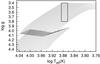Fig. 1 Evolutionary tracks. The rectangle is the 1σ error box for the observational constraints.

3. Stellar models

3.1. Input physics

In this study, we use the so-called package pulse from version 6596 of the Modules for Experiments in Stellar Astrophysics (MESA; Paxton et al. 2011, 2013) to compute stellar evolutionary models and to calculate their pulsation frequencies (Christensen-Dalsgaard 2008). Our theoretical models for HD 50844 are constructed from the ZAMS to the post-main-sequence stage, fully covering the observed ranges of gravitational acceleration and effective temperature. The OPAL equation-of-state tables (Rogers & Nayfonov 2002 ) are used. The OPAL opacity tables from Iglesias & Rogers (1996) are used in the high temperature region and opacity tables from Ferguson et al. (2005) are used in the low temperature region. The T−τ relation of Eddington grey atmosphere is adopted in the atmosphere integration. The mixing-length theory (B$\begin{array}{c}{\mathrm{¨}}_{}\\ \mathrm{o}\end{array}$hm-Vitense 1958) is adopted to treat convection. The effects of convective overshooting and element diffusion are not considered in our calculations.

3.2. Details of model grids

The calibrated value of α = 1.77 for the sun is adopted in our stellar evolutionary models. The evolutionary track of a star on the HR diagram is determined by the stellar mass M and the initial chemical composition (X,Y,Z). In our calculations, we set the initial helium fraction Y = 0.275 as a constant. Then we choose the range of mass fraction of heavy-elements Z from 0.005 to 0.018, to cover the observational value of [Fe/H] = −0.40 ± 0.20 (Poretti et al. 2005).

A grid of stellar models are computed with MESA, M ranging from 1.5 M_⊙ to 2.2 M_⊙ with a step of 0.01 M_⊙, and Z ranging from 0.005 to 0.018 with a step of 0.001. Figure 1 shows the grid of evolutionary tracks with various sets of M and Z. The error box corresponds to the effective temperature range of 7300 K <T_eff< 7700 K and to the gravitational acceleration range of 3.40 < log g< 3.80. For each stellar model falling in the error box, we calculate its frequencies of pulsation modes with l = 0, 1, 2, and 3, and fit them to those observational frequencies according to 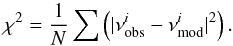${\mathit{\chi }}^{\mathrm{2}}\mathrm{=}\frac{\mathrm{1}}{\mathit{N}}\begin{array}{c}\sum \end{array}\mathrm{\left(}\mathrm{\right|}{\mathit{\nu }}_{\mathrm{obs}}^{\mathit{i}}\mathrm{-}{\mathit{\nu }}_{\mathrm{mod}}^{\mathit{i}}{\mathrm{|}}^{\mathrm{2}}\mathrm{)}\mathit{.}$(2)In Eq. (2), ${\mathit{\nu }}_{\mathrm{obs}}^{\mathit{i}}$ is observational frequency, ${\mathit{\nu }}_{\mathrm{mod}}^{\mathit{i}}$ is the calculated pulsation frequency, and N is the total number of observational frequencies. Based on numerical simulations, most of the uncertainties of the calculated pulsation frequencies are less than 0.03 μHz, except that a few of them reach up to 0.06 μHz.

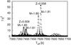Fig. 2 1 /χ2 as a function of the effective temperature Teff. The filled circle denotes the best-fitting model in Sect. 4.1.

4. Analysis of results

4.1. Best-fitting model

In Sect. 2, we give our possible mode identifications for the observed frequencies obtained by Balona (2014) based on the rotational splitting law. When doing model fittings, we try to use the calculated frequencies of each model to fit four identified modes, including two modes with l = 1 (f₂₂ and f₂₉), one mode with l = 2 (f₁₁), and the fundamental radial mode (f₄). Poretti et al. (2009) suggest that f₄ might be one mode with l = 0, based on the mode identifications with the FAMIAS method. Besides, Poretti et al.(2009) detect f₄ in the variations of equivalent width and radial velocity and identified f₄ as the mode with l = 0. Moreover, the photometric identifications made by Poretti et al. (2009) on the basis of the colour information of the multi-colour photometric data show f₄ as the fundamental radial mode. This is in accordance with the property that f₄ has the highest amplitude in the variations of both equivalent width and radial velocity. In our work, we use the identification of f₄ as the fundamental radial mode.

Figure 2 shows the change of 1 /χ² as a function of the effective temperature T_eff for all considered models. In Fig. 2, each curve corresponds to one evolutionary track. In Fig. 2, we note that the value of 1 /χ² is very large in a very small parameter space, i.e., M = 1.80–1.81M_⊙ and Z = 0.008–0.009. Their physical parameters are very close. The physical parameters of HD 50844 are obtained based on these models. These are listed in Table 3. We select the theoretical model with the minimum value of χ² corresponding to (M = 1.81,Z = 0.008) as our best-fitting model, which is indicated with the filled cycle in Fig. 2.

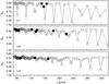Fig. 3 Plot of βk,l to theoretical frequency ν of our best-fitting model. The filled circles denote modes corresponding to the m = 0 mode in Table 5, and the two filled squares denote modes corresponding to the m = 0 modes for Multiplet 8.

The theoretical frequencies of our best-fitting model are listed in Table 4, where n_p is the number of radial nodes in the p-mode propagation region, and n_g the number of radial nodes in the g-mode propagation region. In particular, β_k,l is a parameter measuring the size of rotational splitting for a rigid body in the general formula of rotational splitting derived by Christensen-Dalsgaard (2003): ${\mathit{\beta }}_{\mathit{k,l}}\mathrm{=}\frac{{\mathrm{\int }}_{\mathrm{0}}^{\mathit{R}}\mathrm{(}{\mathit{\xi }}_{\mathit{r}}^{\mathrm{2}}\mathrm{+}\mathit{l}\mathrm{(}\mathit{l}\mathrm{+}\mathrm{1}\mathrm{)}{\mathit{\xi }}_{\mathrm{h}}^{\mathrm{2}}\mathrm{-}\mathrm{2}{\mathit{\xi }}_{\mathit{r}}{\mathit{\xi }}_{\mathrm{h}}\mathrm{-}{\mathit{\xi }}_{\mathrm{h}}^{\mathrm{2}}\mathrm{)}{\mathit{r}}^{\mathrm{2}}\mathit{\rho }\mathrm{d}\mathit{r}}{{\mathrm{\int }}_{\mathrm{0}}^{\mathit{R}}\mathrm{(}{\mathit{\xi }}_{\mathit{r}}^{\mathrm{2}}\mathrm{+}\mathit{l}\mathrm{(}\mathit{l}\mathrm{+}\mathrm{1}\mathrm{\left)}{\mathit{\xi }}_{\mathrm{h}}^{\mathrm{2}}\mathrm{\right)}{\mathit{r}}^{\mathrm{2}}\mathit{\rho }\mathrm{d}\mathit{r}}\mathrm{·}$(3)In Eq. (3), ξ_r is the radial displacement, ξ_h the horizontal displacement, and ρ the local density. Therefore, the effect of rotation is basically determined by the value of β_k,l. For high-order g modes, the terms containing ξ_r can be neglected, thus: ${\mathit{\beta }}_{\mathit{k,l}}\backsimeq \mathrm{1}\mathrm{-}\frac{\mathrm{1}}{\mathit{l}\mathrm{(}\mathit{l}\mathrm{+}\mathrm{1}\mathrm{)}}\mathit{,}$(4)which is in agreement with Eq. (1).

Figure 3 shows the plot of β_k,l versus the theoretical frequency ν for the best-fitting model. It can be seen that most of values of β_k,l in Fig. 3 agree well with the value of 0.5 for l = 1 modes, 0.833 for l = 2 modes, or 0.917 for l = 3 modes derived from Eq. (1). These results indicate that the corresponding modes have pronounced g-mode characteristics. On the other hand, β_k,l of several l = 1, l = 2, and l = 3 modes deviate considerably from the values derived from Eq. (1), indicating that they also possess significant p-mode characteristics.

Table 5 lists the results of comparisons of frequencies for those modes in Table 2, where m ≠ 0 modes in columns named by ν_mod are derived from m = 0 modes, based on P_rot and β_k,l. The filled circles in Fig. 3 denote corresponding m = 0 modes in Table 5. It can be seen clearly in Fig. 3 that values of β_k,l for m = 0 modes corresponding to f₂₂, f₂₉, f₁₁, f₁, f₁₅, and f₃₄ agree well with those derived from Eq. (1). In Multiplet 7, 8, 9, 11, and 2, m = 0 components are not observed. Values of β_k,l for corresponding m = 0 components in Multiplet 7, 9, 11, and 12 are also in good agreement with those derived form Eq. (1). The mode corresponding to f₂₅ in Multiplet 3 and corresponding m = 0 component in Multiplet 10 have slightly larger values of β_k,l than those derived from Eq. (1). It can be noticed in Table 5 that there are two possible identifications for Multiplet 8, i.e., corresponding to modes of m = (−1, + 2) derived from 80.189 μHz (2, 0, −78, 0), or m = (−2, + 1) from 84.368 μHz (2, 0, −74, 0). The filled squares in Fig. 3 denote these two possible m = 0 modes in Multiplet 8. It can be seen in Fig. 3 that the values of β_k,l for both of the two choices are in good agreement with Eq. (1). These results confirm our approach of using Eq. (1) to search for rotational splitting in Sect. 2.

Based on the best-fitting model, possible identifications for f₁₃, f₁₆, f₃₀, f₃₁, f₃₂, and f₄₀ are listed in Table 6. In Table 6, we note that f₃₀, f₃₁, f₃₂, and f₄₀ may be identified as four modes with l = 3. et al. (2009) identify f₃₀ as (l = 4,m = 2) and f₃₁ as (l = 4,m = 3). Considering uncertainties of spectroscopic observations obtained by (Poretti et al. 2009), the spherical harmonic degree l of our suggestions agree with those of Poretti et al. (2009). For f₁₆, there are three possible identifications, i.e., corresponding to modes of (l,m) =(2,−2), (3, + 2), or (3,0). Besides, there are two possible identifications for f₁₅ based on the analyses in Sect. 2. If f₁₅ and f₁₃ are identified as two components of one incomplete septuplet, (130.081,134.465) derived from 138.850 μHz (3,2,−62,0) or (130.035,134.392) derived from 143.104 μHz (3,2,−60,0) may be two possibilities. If f₁₅ and f₁₈ are identified as two components of one incomplete quintuplet, the results of comparisons are listed in Table 5. Poretti et al. (2009) identified f₁₅ as a mode with (l = 8, m = 5). The spherical harmonic degree l for both of the two cases (l = 3 or 2) are lower than the value of Poretti et al. (2009).

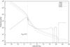Fig. 4 N denotes Brunt−V$\begin{array}{c}{\mathrm{¨}}_{}\\ \mathrm{a}\end{array}$is$\begin{array}{c}{\mathrm{¨}}_{}\\ \mathrm{a}\end{array}$l$\begin{array}{c}{\mathrm{¨}}_{}\\ \mathrm{a}\end{array}$ frequency and Ll (l = 1,2,3) denote Lamb frequency. M∗ denotes the total mass of the star. The vertical line denotes the boundary of the helium core.

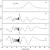Fig. 5 Scaled eigenfunctions of modes corresponding to f4, f11, f22, and f29. ${\mathit{X}}_{\mathit{q}}\mathrm{=}\sqrt{\mathit{q}\mathrm{(}\mathrm{1}\mathrm{-}\mathit{q}\mathrm{)}}$ and q = Mr/M∗. Panel a) is for the fundamental radial mode 79.937 μHz (l = 0,np = 0,ng = 0). Panel b) is for the mode 151.060 μHz (l = 1,np = 3,ng = −23). Panel c) is for the mode 164.999 μHz (l = 1,np = 4,ng = −21). Panel d) is for the mode 123.113 μHz (l = 2,np = 2,ng = −50). Vertical line denotes the boundary of the helium core.

4.2. Discussions

An important question to address is why physical parameters of HD 50844 are well limited in a small region based on four identified pulsation modes. We have found a possible reason to explain this result.

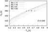Fig. 6 Plot of sound radius Th to period spacing Π0 with the same initial metallicity Z = 0.008 and different stellar mass M. The filled circle represents our best-fitting model. The filled triangles represent models that have a minimum value of χ2 on corresponding evolutionary tracks.

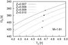Fig. 7 Plot of sound radius Th to period spacing Π0 with the same stellar mass M = 1.81 and different initial metallicity Z. The filled circle represents our best-fitting model. The filled triangles represent models which have a minimum value of χ2 on corresponding evolutionary tracks.

First of all, we note that the four identified modes consist of two l = 1 modes (f₂₂ and f₂₉), one l = 2 mode (f₁₁), and the fundamental radial mode (f₄). Table 4 shows that most of the pulsation modes are mixed modes. Figure 4 shows the propagation diagram for the best-fitting model. According to the parameter settings of MESA (Paxton et al. 2011, 2013), the boundary of helium core is set to the position where the hydrogen fraction X_cb = 0.01. The vertical lines in Figs. 4 and 5 denote the position of the boundary of the helium core. The inner zone is the helium core, the outer zone is the stellar envelope. In Fig. 4, we see that the Brunt-V$\begin{array}{c}{\mathrm{¨}}_{}\\ \mathrm{a}\end{array}$is$\begin{array}{c}{\mathrm{¨}}_{}\\ \mathrm{a}\end{array}$l$\begin{array}{c}{\mathrm{¨}}_{}\\ \mathrm{a}\end{array}$ frequency N has a peak in the helium core, which corresponds to the hydrogen-burning shell. Figure 5 shows distributions of the radial displacement for the fundamental radial mode and the three nonradial modes that we have considered. In Fig. 5, we clearly see that the fundamental radial mode propagates mainly in the stellar envelope, and represents the property of the stellar envelope. However, the three nonradial modes propagate like g modes in the helium core while like p modes in the stellar envelope. This fact confirms that they are mixed modes and can therefore represent the property of the helium core. To fit those four modes at the same time, both the stellar envelope and the helium core must be matched to the considered star.

The acoustic radius T_h is defined as T_h = ${{}^{\mathrm{\int }}}_{\mathrm{0}}^{\mathit{R}}{\mathit{c}}_{\mathrm{s}}^{-1}\mathrm{d}\mathit{r}$ (Aerts et al. 2010), where c_s is the adiabatic sound speed. Therefore, the acoustic radius T_h is mainly determined by the distribution of c_s inside the star. The sound speed c_s is much smaller in the stellar envelope than in the helium core, thus T_h can be used to reflect the property of the stellar envelope.

According to the asymptotic theory of g modes, there is an equation for the period separation (Unno et al. 1979; Tassoul 1980) 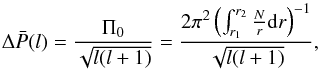$\mathrm{\Delta }\mathit{P̅}\mathrm{\left(}\mathit{l}\mathrm{\right)}\mathrm{=}\frac{{\mathrm{\Pi }}_{\mathrm{0}}}{\sqrt{\mathit{l}\mathrm{(}\mathit{l}\mathrm{+}\mathrm{1}\mathrm{)}}}\mathrm{=}\frac{\mathrm{2}{\mathit{\pi }}^{\mathrm{2}}{\left({\mathrm{\int }}_{{\mathit{r}}_{\mathrm{1}}}^{{\mathit{r}}_{\mathrm{2}}}\frac{\mathit{N}}{\mathit{r}}\mathrm{d}\mathit{r}\right)}^{-1}}{\sqrt{\mathit{l}\mathrm{(}\mathit{l}\mathrm{+}\mathrm{1}\mathrm{)}}}\mathit{,}$(5)where r₁ is the inner boundary of the region where gravity waves propagate, r₂ is the outer boundary, and N is the Brunt-V$\begin{array}{c}{\mathrm{¨}}_{}\\ \mathrm{a}\end{array}$is$\begin{array}{c}{\mathrm{¨}}_{}\\ \mathrm{a}\end{array}$l$\begin{array}{c}{\mathrm{¨}}_{}\\ \mathrm{a}\end{array}$ frequency. In Eq. (5), ${\mathrm{\Pi }}_{\mathrm{0}}\mathrm{=}\mathrm{2}{\mathit{\pi }}^{\mathrm{2}}\mathrm{(}{{}^{\mathrm{\int }}\mathit{r}_{\mathrm{1}}}_{{\mathit{r}}_{\mathrm{2}}}^{}\mathit{N}\mathit{/}\mathit{r}\mathrm{d}\mathit{r}{\mathrm{)}}^{-1}$, which is mainly determined by the distribution of Brunt-V$\begin{array}{c}{\mathrm{¨}}_{}\\ \mathrm{a}\end{array}$is$\begin{array}{c}{\mathrm{¨}}_{}\\ \mathrm{a}\end{array}$l$\begin{array}{c}{\mathrm{¨}}_{}\\ \mathrm{a}\end{array}$ frequency N in the helium core. Therefore, Π₀ can be used to reflect the property of the helium core.

Figure 6 shows the distribution of the period spacing Π₀ versus the acoustic radius T_h for theoretical models with the same initial metallicity Z but different stellar mass M. Figure 7 shows the same plot for theoretical models with the same stellar mass M, but different initial metallicity Z. The filled circle corresponds to our best-fitting model, while the filled triangles correspond to stellar models having minimum values of χ² on the corresponding evolutionary tracks, respectively. In Fig. 6, we note that the acoustic radius T_h of the stellar models marked by the filled triangles obviously deviate from the value of our best-fitting model, which indicates that the stellar envelopes of these models cannot match the actual structure of the considered star. In contrast, the period spacing Π₀ of the stellar models indicated by the filled triangles in Fig. 7 obviously deviate from the value of our best-fitting model, which indicates that the helium cores of these models cannot match the actual structure of the considered star. Based on the above arguments, further more the size of the helium core of the δ Scuti star HD 50844 is determined for the first time. The corresponding physical parameters are listed in Table 3.

Gizon & Solanki (2003) investigated in details the relation between the stellar oscillation amplitude and the inclination angle i of stellar rotation axes. In Table 1, we can see that the m = 0 component f₂₂ of Multiplet 1 has an amplitude that is about nine times smaller than the m = −1 components f₂₁ and about seven times smaller than the m = + 1 components f₂₃. Such large differences correspond to an inclination angle i ≈ 76° according to the relation given by Gizon & Solanki (2003). This fact is roughly in agreement with the value of 82° (Poretti et al. 2009). The m = 0 component in Multiplet 4 has the least amplitude, and the m = 0 component in Multiplet 2 also has a smaller amplitude.

The rotational period P_rot is determined as being 2.44$\begin{array}{c}\mathrm{+}\mathrm{0.13}\\ -0.08\end{array}$ days according to Eq. (1). In Table 3, we note that the theoretical radius of HD 50844 is R = 3.300 ± 0.023 R_⊙. As such, the rotational velocity at the equator is derived as υ_rot = 68.33$\begin{array}{c}\mathrm{+}\mathrm{2.34}\\ -3.70\end{array}$ km s^-1 according to υ_rot = 2πR/P_rot. Assuming the inclination angle i = 82 ± 4 deg (Poretti et al. 2009), υ_rotsini is estimated to be 66.86 ± 3.64 km s^-1, which is higher than the value of υsini = 58 ± 2 km s^-1 (Poretti et al. 2009). In Sect. 4.1, we demonstrated that most of the considered frequencies are mixed modes. They have pronounced g-mode characteristics. The corresponding rotational velocity derived from rotational splitting of these modes mainly reflects the rotational properties of the helium core. The δ Scuti star HD 50844 is a slightly evolved star. As the star evolves into the post-main-sequence stage, the core shrinks and the envelope expands. Based on the conservation of angular momentum, rotational angular velocity of the core should be larger than that of the envelope. The spectroscopic value of υsini (Poretti et al. 2009) mainly reflects the property of the envelope. This may be the reason why our rotational velocity is higher than that of Poretti et al. (2009).

5. Summary

In our work, we have analysed the observed frequencies given by Balona (2014) for possible rotational splitting, and carried out numerical model fittings for the δ Scuti star HD 50844. We summarize our results as follows:

We identify two complete triplets (f₂₁, f₂₂, f₂₃) and (f₂₇, f₂₉, f₃₃) as modes with l = 1, and one incomplete quintuplet (f₉, f₁₁, f₁₄) as modes with l = 2, as well as one more incomplete triplet (f₂₄, f₂₅) as modes with l = 1 and six more incomplete quintuplets (f₁, f₅), (f₁₅, f₁₈), (f₃₅, f₃₆), (f₂, f₇), (f₁₂, f₂₀), and (f₃₈, f₃₉) as modes with l = 2. Besides, three incomplete septuplets (f₃,f₆,f₈), (f₁₀,f₁₇,f₁₉), and (f₂₆,f₂₈,f₃₄,f₃₇) are identified as modes with l = 3. Based on frequency differences of the above multiplets, the corresponding rotational period of HD 50844 is found to be 2.44$\begin{array}{c}\mathrm{+}\mathrm{0.13}\\ -0.08\end{array}$ days.

Based on our model calculations, we compare theoretical pulsation modes with four identified observational modes, including three nonradial modes (f₁₁, f₂₂, f₂₉) and the fundamental radial mode (f₄). The physical parameters of HD 50844 are well limited in a small region. Based on the fitting results, we suggest the theoretical model with M = 1.81M_⊙, Z = 0.008 as the best-fitting model.

Based on our best-fitting model, we find that the values of β_k,l for most of the calculated modes are in good agreement with the asymptotic values for g-modes. Some modes may have values of β_k,l that are considerably higher than the asymptotic values. However, the values of β_k,l for the m = 0 modes in those identified triplets, quintuplets, or septuplets are in good agreement with the asymptotic values of g-modes, which confirms that our approach for searching for rotational splitting based on the rule of g-modes is self-consistent.

Based on comparisons of all observed frequencies with their theoretical counterparts, we find that most of the considered frequencies may belong to mixed modes. The radial fundamental mode f₄ reflects the property of the stellar envelope, while the three nonradial modes f₁₁, f₂₂, and f₂₉ reflect the property of the helium core. These features require that both the stellar envelope and the helium core must be matched to the actual structure to fit these four oscillation modes. Finally, the mass of helium core of HD 50844 is estimated to be 0.173 ± 0.004 M_⊙.

Acknowledgments

We are sincerely grateful to an anonymous referee for instructive advice and productive suggestions that greatly helped us to improve the manuscript. This work is funded by the NSFC of China (Grant No. 11333006, 11521303, and 11403094) and by the foundation of Chinese Academy of Sciences (Grant No. XDB09010202 and Light of West China Program). We gratefully acknowledge the computing time granted by the Yunnan Observatories, and provided on the facilities at the Yunnan Observatories Supercomputing Platform. We are also very grateful to J.-J. Guo, G.-F. Lin, Q.-S. Zhang, Y.-H. Chen, and J. Su for their kind discussions and suggestions.

References

All Tables

All Figures

	Fig. 1 Evolutionary tracks. The rectangle is the 1σ error box for the observational constraints.
In the text

	Fig. 2 1 /χ2 as a function of the effective temperature Teff. The filled circle denotes the best-fitting model in Sect. 4.1.
In the text

	Fig. 3 Plot of βk,l to theoretical frequency ν of our best-fitting model. The filled circles denote modes corresponding to the m = 0 mode in Table 5, and the two filled squares denote modes corresponding to the m = 0 modes for Multiplet 8.
In the text

	Fig. 4 N denotes Brunt−V$\begin{array}{c}{\mathrm{¨}}_{}\\ \mathrm{a}\end{array}$is$\begin{array}{c}{\mathrm{¨}}_{}\\ \mathrm{a}\end{array}$l$\begin{array}{c}{\mathrm{¨}}_{}\\ \mathrm{a}\end{array}$ frequency and Ll (l = 1,2,3) denote Lamb frequency. M∗ denotes the total mass of the star. The vertical line denotes the boundary of the helium core.
In the text

Fig. 5 Scaled eigenfunctions of modes corresponding to f4, f11, f22, and f29. ${\mathit{X}}_{\mathit{q}}\mathrm{=}\sqrt{\mathit{q}\mathrm{(}\mathrm{1}\mathrm{-}\mathit{q}\mathrm{)}}$ and q = Mr/M∗. Panel a) is for the fundamental radial mode 79.937 μHz (l = 0,np = 0,ng = 0). Panel b) is for the mode 151.060 μHz (l = 1,np = 3,ng = −23). Panel c) is for the mode 164.999 μHz (l = 1,np = 4,ng = −21). Panel d) is for the mode 123.113 μHz (l = 2,np = 2,ng = −50). Vertical line denotes the boundary of the helium core.

In the text

	Fig. 6 Plot of sound radius Th to period spacing Π0 with the same initial metallicity Z = 0.008 and different stellar mass M. The filled circle represents our best-fitting model. The filled triangles represent models that have a minimum value of χ2 on corresponding evolutionary tracks.
In the text

	Fig. 7 Plot of sound radius Th to period spacing Π0 with the same stellar mass M = 1.81 and different initial metallicity Z. The filled circle represents our best-fitting model. The filled triangles represent models which have a minimum value of χ2 on corresponding evolutionary tracks.
In the text

References

- Aerts, C., Christensen-Dalsgaard, J., & Kurtz, D. W. 2010, Asteroseismology, 1st edn. (Springer), 866 [Google Scholar]
- Baker, N., & Kippenhahn, R. 1962, Z. Astrophys., 54, 114 [NASA ADS] [Google Scholar]
- Baker, N., & Kippenhahn, R. 1965, ApJ, 142, 868 [NASA ADS] [CrossRef] [Google Scholar]
- Balona, L. A. 2014, MNRAS, 439, 3453 [NASA ADS] [CrossRef] [Google Scholar]
- Breger, M., Handler, G., Garrido, R., et al. 1999, A&A, 349, 225 [NASA ADS] [Google Scholar]
- Breger, M., Lenz, P., Antoci, V., et al. 2005, A&A, 435, 955 [NASA ADS] [CrossRef] [EDP Sciences] [Google Scholar]
- Breger, M. 2000, ASP Conf. Ser., 210, 3 [Google Scholar]
- Böhm-Vitense, E. 1958, Z. Astrophys., 46, 108 [Google Scholar]
- Castanheira, B. G., Breger, M., Beck, P. G., et al. 2008, Commun. Asteroseismol., 157, 124 [NASA ADS] [Google Scholar]
- Christensen-Dalsgaard, J. 2003, Lecture notes on Stellar Oscillations, 5th edn. (Institut for Fysik og Astronomi, Aarhus Universitet) [Google Scholar]
- Christensen-Dalsgaard, J. 2008, Ap&SS, 316, 113 [NASA ADS] [CrossRef] [Google Scholar]
- Civelek, R., Kızıloǧlu, N., & Kırbıyık, H. 2001, AJ, 122, 2042 [NASA ADS] [CrossRef] [Google Scholar]
- Daszyńska-Daszkiewicz, J., Dziembowski, W. A., Pamyantykh, A. A., et al. 2005, A&A, 438, 653 [NASA ADS] [CrossRef] [EDP Sciences] [Google Scholar]
- Deupree, R. G., Castañeda, D., Peña, F., & Short, C. I. 2012, APJ, 753, 20 [NASA ADS] [CrossRef] [Google Scholar]
- Dziembowski, W. A., & Goode, P. R. 1992, APJ, 394, 670 [Google Scholar]
- Ferguson, J. W., Alexander, D. R., Allard, F., et al. 2005, ApJ, 623, 585 [NASA ADS] [CrossRef] [Google Scholar]
- García Hernández, A., Moya, A., Michel, E., et al. 2013, A&A, 559, A63 [NASA ADS] [CrossRef] [EDP Sciences] [Google Scholar]
- Garrido, R., Suarez, J. C., Grigahcene, A., et al. 2007, Commun. Asteroseismol., 150, 77 [Google Scholar]
- Gizon, L., & Solanki, S. K. 2003, APJ, 589, 1009 [CrossRef] [Google Scholar]
- Iglesias, C. A., & Rogers, F. J. 1996, ApJ, 464, 943 [NASA ADS] [CrossRef] [Google Scholar]
- Kırbıyık, H., Civelek, R., & Kızıloǧlu, N. 2003, Ap&SS, 288, 305 [NASA ADS] [CrossRef] [Google Scholar]
- Lenz, P., Pamyatnykh, A. A., Breger, M., & Antoci, V. 2008, A&A, 478, 855 [NASA ADS] [CrossRef] [EDP Sciences] [Google Scholar]
- Lenz, P., Pamyatnykh, A. A., Zdravkov, T., & Breger, M. 2010, A&A, 509, A90 [NASA ADS] [CrossRef] [EDP Sciences] [Google Scholar]
- Li, Y., & Stix, M. 1994, A&A, 286, 815 [NASA ADS] [Google Scholar]
- Lignières, F., Rieutord, M., & Reese, D. 2006, A&A, 455, 607 [NASA ADS] [CrossRef] [EDP Sciences] [Google Scholar]
- Mantegazza, L. 1997, A&A, 323, 844 [NASA ADS] [Google Scholar]
- Mantegazza, L. 2000, ASP Conf. Ser., 210, 138 [Google Scholar]
- Mantegazza, L., Poretti, E., & Zerbi, F. M. 2001, A&A, 366, 547 [NASA ADS] [CrossRef] [EDP Sciences] [Google Scholar]
- Mantegazza, L., Poretti, E., Michel, E., et al. 2012, A&A, 542, A24 [NASA ADS] [CrossRef] [EDP Sciences] [Google Scholar]
- Paxton, B., Bildsten, L., Dotter, A., et al. 2011, ApJS, 192, 3 [Google Scholar]
- Paxton, B., Cantiello, M., Arras, P., et al. 2013, ApJS, 208, 4 [NASA ADS] [CrossRef] [Google Scholar]
- Poretti, E., Alonso, R., Amado, P. J., et al. 2005, AJ, 129, 2461 [NASA ADS] [CrossRef] [Google Scholar]
- Poretti, E., Michel, E., Garrido, R., et al. 2009, A&A, 506, 85 [NASA ADS] [CrossRef] [EDP Sciences] [Google Scholar]
- Rogers, F. J., & Nayfonov, A. 2002, ApJ, 576, 1064 [Google Scholar]
- Schmid, V. S., Themeβl, N., Breger, M., et al. 2014, A&A, 570, A33 [NASA ADS] [CrossRef] [EDP Sciences] [Google Scholar]
- Tassoul, M. 1980, ApJS, 43, 469 [NASA ADS] [CrossRef] [Google Scholar]
- Unno, W., Osaki, Y., Ando, H., & Shibahashi, H. 1979, Nonraidal oscillations of stars (University of Tokyo Press) [Google Scholar]
- Winget, D. E., Nather, R. E., Clemens, J. C., et al. 1991, ApJ, 378, 326 [NASA ADS] [CrossRef] [Google Scholar]
- Zhao, M., Monnier, J. D., Pedretti, E., et al. 2009, ApJ, 701, 209 [NASA ADS] [CrossRef] [Google Scholar]
- Zhevakin, S. A. 1963, ARA&A, 1, 367 [NASA ADS] [CrossRef] [Google Scholar]
- Zima, W. 2008, Commun. Asteroseismol., 155, 17 [Google Scholar]
- Zima, W., Wright, D., Bentley, J., et al. 2006, A&A, 455, 235 [NASA ADS] [CrossRef] [EDP Sciences] [Google Scholar]
All Tables
Possible mode identifications for the rest of the observed frequencies based on our best-fitting model.