| Issue |
A&A
Volume 593, September 2016
|
|
|---|---|---|
| Article Number | A89 | |
| Number of page(s) | 12 | |
| Section | Extragalactic astronomy | |
| DOI | https://doi.org/10.1051/0004-6361/201527393 | |
| Published online | 28 September 2016 | |
Magnetic fields during galaxy mergers
1 Max-Planck-Institute for Solar System Research, Justus-von-Liebig-Weg 3, 37077 Göttingen, Germany
e-mail: This email address is being protected from spambots. You need JavaScript enabled to view it.
2 Departamento de Astronomía, Facultad Ciencias Físicas y Matemáticas, Universidad de Concepción, Av. Esteban Iturra s/n Barrio Universitario, Casilla 160-C, Concepción, Chile
e-mail: This email address is being protected from spambots. You need JavaScript enabled to view it.
Received: 17 September 2015
Accepted: 30 June 2016
Abstract
Galaxy mergers are expected to play a central role for the evolution of galaxies and may have a strong effect on their magnetic fields. We present the first grid-based 3D magnetohydrodynamical simulations investigating the evolution of magnetic fields during merger events. For this purpose, we employed a simplified model considering the merger event of magnetized gaseous disks in the absence of stellar feedback and without a stellar or dark matter component. We show that our model naturally leads to the production of two peaks in the evolution of the average magnetic field strength within 5 kpc, within 25 kpc, and on scales in between 5 and 25 kpc. The latter is consistent with the peak in the magnetic field strength previously reported in a merger sequence of observed galaxies. We show that the peak on the galactic scale and in the outer regions is most likely due to geometrical effects, as the core of one galaxy enters the outskirts of the other one. In addition, the magnetic field within the central ~5 kpc is physically enhanced, which reflects the enhancement in density that is due to efficient angular momentum transport. We conclude that high-resolution observations of the central regions will be particularly relevant for probing the evolution of magnetic field structures during merger events.
Key words: Galaxy: evolution / galaxies: interactions / galaxies: magnetic fields / methods: numerical
© ESO, 2016
1. Introduction
Galaxy mergers are central for the evolution of galaxies and have a strong influence on many of their properties. In a pioneering study to investigate the impact of mergers, Toomre (1977) has proposed a merging sequence of 11 peculiar galaxies spanning a range of pre- and post-mergers that became known as the Toomre sequence. This sequence suggested that the final product of mergers resembles an elliptical galaxy. This behavior was confirmed by numerical simulations following the N-body dynamics of the stellar population, finding the characteristic formation of r1/4 profiles observed in elliptical galaxies (Barnes 1988, 1992; Hernquist 1992, 1993; Privon et al. 2013). Observational studies have provided evidence for this scenario, reporting a characteristic r1/4 profile in merger remnants (Joseph & Wright 1985) and finding low surface brightness loops and shells in elliptical galaxies, which are likely the remnants from previous mergers (Malin & Carter 1980; Schweizer & Seitzer 1988). Forbes et al. (1998) have shown that late-stage disk-disk mergers and ellipticals with young stellar populations deviate from the fundamental plane of elliptical galaxies as a result of a centrally located starburst induced by the merger event.
Gravitational instabilities acting during the merger event may channel significant gas flows toward the center of the galaxy, enhancing the activity of star formation or of a central supermassive black hole (Mihos & Hernquist 1996). High molecular gas fractions have been observed in IRAS starburst galaxies, which are considered as gas-rich systems close to the final stages of merging (Sanders & Mirabel 1996; Planesas et al. 1997; Kennicutt 1998). The enhanced star-formation activity has been confirmed both in the far-infrared (Kennicutt 1998) and in the radio (Hummel 1981; Hummel et al. 1990) and the optical (Keel et al. 1985). Near-infrared observations with the Hubble Space Telescope show a distinct trend for the nuclei to become more luminous in more advanced merging stages (Rossa et al. 2007). Similarly, the fraction of interacting systems in IRAS-selected samples increases with far-infrared luminosity (Lawrence et al. 1989; Gallimore & Keel 1993).
Gao & Solomon (1999) have used the projected separation between the nuclei of merging galaxies as an estimator for the interaction stage, finding clear evidence for increasing star formation efficiencies, which is defined by the ratio of far-infrared luminosity to molecular hydrogen mass, with decreasing spatial separation. The latter potentially indicates more efficient star formation in higher-density gas. The increase of star formation activity during the merger event is also reflected in X-ray observations (Read & Ponman 1998; Brassington et al. 2007) and in the UV (Smith et al. 2010). Hibbard & van Gorkom (1996) investigated the cold gas properties from a small sample of pre- and post-mergers, finding strong differences in the HI distribution in pre- and post-mergers, with increasing fractions of HI outside the optical bodies toward the later stages. They proposed that the latter is due to the ejection of cold gas in tidal features.
Georgakakis et al. (2000) investigated a sample of 53 interacting galaxy pairs by combining radio observations with optical data by Keel & Wu (1995), far-infrared data by Gao & Solomon (1999), and 60μm data from the sample of Surace et al. (1993) based on the IRAS Bright Galaxy Sample (Soifer et al. 1987). They defined the interaction parameter in terms of the effective age before or after the merger, confirming a significant increase of the star formation efficiency during the merger event. The latter is reflected in a correlation between the star formation efficiency and the H2 surface density. The amount of molecular gas is found to increase during the merger as well, and to fall off after the merger. Beyond the statistical samples, some interacting galaxy pairs have been studied in particular detail. For instance, the Antennae galaxies (NGC 4038/39) have been explored with Chandra in the X-rays (Fabbiano et al. 2001), with Herschel-PACS, revealing obscured star formation (Klaas et al. 2010), and with the Submillimeter Array pursuing high-resolution CO observations (Ueda et al. 2012). The change of the gas distribution due to the merger event may also be relevant for the cosmological growth of black holes (Mayer et al. 2010; Treister et al. 2012; Ferrara et al. 2013; Capelo et al. 2015).
In addition to star formation and the molecular gas, magnetic fields are a relevant component of galaxies that can influence the star formation rate (e.g., Banerjee et al. 2009; Vázquez-Semadeni et al. 2011; Federrath & Klessen 2012). The structure of the galactic magnetic field has been studied in detail in nearby galaxies (e.g., Beck et al. 1999, 2005; Fletcher et al. 2011; Tabatabaei et al. 2013; Heesen et al. 2014). More recently, the presence of magnetic fields was also confirmed in nearby dwarf galaxies (Chyży et al. 2000, 2011; Kepley et al. 2010, 2011; Heesen et al. 2011). The far-infrared − radio correlation suggests that the presence of magnetic fields is strongly correlated with star formation activity, where the magnetic field strength B scales approximately as the star formation surface density ΣSFR to the one third (de Jong et al. 1985; Helou et al. 1985; Niklas & Beck 1997; Yun et al. 2001; Basu et al. 2012; Schleicher & Beck 2013), and this has also been confirmed at high redshift (Murphy 2009; Jarvis et al. 2010; Ivison & et. al. 2010; Bourne et al. 2011; Casey et al. 2012). Prospects for probing the far-infrared − radio correlation at high redshift and in nearby dwarf galaxies at low star formation rates have been formulated by Schleicher & Beck (2016) and Schober et al. (2016).
While radio data have been available for interacting galaxy pairs early on (e.g., Condon 1983; Condon et al. 1993, 2002), the first detailed analysis of the magnetic field structure in an interacting galaxy pair has been pursued by Chyży & Beck (2004) for the Antennae galaxies. With ~20μG, the mean total magnetic field strength is significantly greater than in isolated spirals and might be enhanced through interaction-induced star formation. The field regularity appears to be lower than in isolated galaxies, reflecting additional distortions or feedback related to star formation. The observed structures are roughly consistent with magnetohydrodynamical (MHD) simulations by Kotarba et al. (2010) based on a smoothed particle hydrodynamics (SPH) aproach. The galaxy pair NGC 2207/IC 2163 has been observed in the optical by Elmegreen et al. (1995b) and was modeled with N-body simulations by Elmegreen et al. (1995a), which were able to reproduce the main dynamical features. The radio emission at 4.86 GHz covers the optical extent of the system, but includes a hole in the central part of NGC 2207 (Condon 1983). For the Taffy (UGC 12914/15), a galaxy pair with a nearly head-on encounter, a significant amount of data is available, including radio and HI (Condon et al. 1993) as well as CO and the dust continuum (Gao et al. 2003; Zhu et al. 2007). A similar pair of post-collision spiral galaxies, UGC 813/16, was detected at 1.40 GHz and forms the so-called Taffy2 (Condon et al. 2002).
The first more systematic study of magnetic fields in a complete merging sequence has been pursued by Drzazga et al. (2011). For this purpose, they compiled a sample of data from the Very Large Array (VLA) based on the merging sequence of Toomre (1977) and Brassington et al. (2007) and other interacting systems, leading to a total of 24 interacting galaxy pairs, including pre- and post-merger stages. While they did not consider them a complete sample of colliding galaxies, these pairs represent the different stages of tidal interaction and merging. For this sample, a correlation of the average magnetic field strength in the whole galaxy and in the central region is found with the star formation surface density ΣSFR. The central magnetic field strength scales as  , consistent with the scaling relations in spiral galaxies (Niklas & Beck 1997), and Drzazga et al. (2011) reported that their sample lies on the far-infrared − radio correlation for spiral galaxies.
The evolution of magnetic fields during merger events is also interesting from a theoretical point of view because the merger process leads to the production of turbulence, which can enhance the small-scale magnetic fields through the small-scale dynamo (e.g., Schekochihin et al. 2002; Cho et al. 2009; Federrath et al. 2011; Schober et al. 2012, 2015; Schleicher et al. 2013; Bhat & Subramanian 2014) and also affect the formation of a large-scale field through dynamo processes (Ruediger & Kichatinov 1993; Brandenburg & Subramanian 2005; Gressel et al. 2013; Park et al. 2013). The number of numerical simulations exploring such merger scenarios is still limited, however. Beyond the MHD-SPH simulations of the Antennae galaxies pursued by Kotarba et al. (2010), the effect of multiple mergers has been explored with the same approach by Kotarba et al. (2011). Magnetic field amplification during minor galaxy mergers has been investigated with a similar approach by Geng et al. (2012). Grid-based simulations of merging systems have been pursued in a 2D-approximation by Moss et al. (2014). However, as turbulence is essentially a 3D phenomenon, it is desireable to explore the evolution of magnetic fields during merger events with three-dimensional grid-based techniques.
In this paper we present a toy model to explore 3D effects during the merger of magnetized gaseous disks. While this model still neglects the effect of the dark matter on the merger events, it shows that geometric projection events can be rather important when interpreting large-scale averages in observations of magnetic fields. We show through a parameter study that the occurrence of characteristic peaks that are due to projection effects is rather insensitive to the details of the orbit. Our simulation setup is presented in Sect. 2 and the main results are given in Sect. 3. We show that our simulations can already reproduce some of the main features in the merger sequence by Drzazga et al. (2011). Our results and their implications for the interpretation of observational data are discussed in Sect. 4.
2. Simulation setup
Our simulations were pursued with the publicly available MHD adaptive mesh-refinement (AMR) code Enzo1 (O’Shea et al. 2004; Bryan et al. 2014). To solve the MHD equations, we employed the monotonic upstream-centered scheme for conservation laws (MUSCLE; van Leer 1979) with the divergence-cleaning scheme developed by Dedner et al. (2002). The latter was implemented in the Enzo code by Wang & Abel (2009). In this approach, the divergence of B is kept small through an additional damping term. The latter is slightly less accurate than the constrained transport approach employed by Collins et al. (2010), but computationally more efficient, which is highly beneficial for the merger simulations pursued here.
In our numerical setup, we consider the collision of two magnetized gaseous disks as a toy model to investigate the evolution of magnetic fields during merger events. In particular, we neglect here the potential effect of a dark matter halo and the stellar component. While the latter provides an external potential that might be able to stabilize the disk, we expect that the qualitative evolution of the magnetic fields will not strongly depend on their effects. Similarly, the additional presence of a dark matter halo would stabilize the galaxy against tidal effects and increase both the gravitational and the inertial mass, while the dynamical friction due to the dark matter is most likely reduced compared to the baryons. The initial conditions of the disks are based on the isolated disk models by Wang et al. (2010) and Braun et al. (2014).
2.1. Gas distribution
We considered an exponential gaseous disk where the surface density is given as (1)with R the characteristic length scale of the disk and Σ0 the surface density in the center. For the vertical density profile, we considered a distribution
 (2)where H(r) is the scale height of the disk at radius r. In the following, we adopt the abbreviation ρ0(r) = ρ(r,z = 0). Assuming that the self-gravity of the disk is balanced by gas pressure, the scale height is given as
 (3)where G is the gravitational constant, cs(r) the local sound speed, and ϵmag denotes the ratio of magnetic to thermal pressure, which is assumed to be constant in the initial condition. In the following we assume a constant gas temperature in the initial condition and thus also a constant sound speed cs. Through an integration of Eq. (1), the total mass in the disk is given as
  (4)For a given mass of the disk, the normalization constant Σ0 thus follows as
 (5)For the disk density profile in Eq. (2), we have the following identity:
  (6)Comparing Eqs. (1) and (6) and inserting the expression (5), we can show that
 (7)As a result, the density distribution is given as
 (8)While the above considerations assume a balance between gravity and thermal pressure, the approach given by Wang et al. (2010) can be extended for additional nonthermal pressure components, including magnetic pressure. For this purpose, we adopted the following system of equations:
![Mathematical equation: \begin{eqnarray} \frac{{\rm d}^2\Phi}{{\rm d}z^2}&=&4\pi G\rho(r,z),\\ \rho(r,z)&=&\rho_0(r)\mathrm{exp}\left( \Phi_z(r,z)\left[ \left( \frac{{\rm d}\rho}{{\rm d}z} \right)^{-1}\frac{{\rm d}p}{{\rm d}z} \right]^{-1} \right),\\ \rho_0(r)&=&\frac{\Sigma_0 \mathrm{exp}\left( -\frac{r}{R} \right)}{2\int_0^\infty \mathrm{exp}\left( \Phi_z(r,z)\left[ \left( \frac{{\rm d}\rho}{{\rm d}z} \right)^{-1} \frac{{\rm d}p}{{\rm d}z} \right]^{-1} \right){\rm d}z}, \end{eqnarray}](/articles/aa/full_html/2016/09/aa27393-15/aa27393-15-eq36.png) with Φz = Φ(r,z) − Φ(r,0). This system of equations is solved through an iterative approach, starting with an initial guess for ρ0(r) based on the solution neglecting the magnetic pressure. The method typically converges within a few iterations.
with Φz = Φ(r,z) − Φ(r,0). This system of equations is solved through an iterative approach, starting with an initial guess for ρ0(r) based on the solution neglecting the magnetic pressure. The method typically converges within a few iterations.
2.2. Velocity field
For galactic disks in which the surface density Σ(r) follows an exponential profile, an analytical solution describes the case where the gravitational force is completely balanced by rotation (Freeman 1970):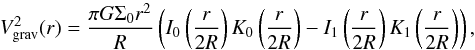 (12)where Ii and Ki are the modified Bessel functions of order i. In a realistic disk, the gravitational force is not only balanced by the centrifugal force, however, but also by thermal and magnetic pressure. To take this into account, the rotational velocity is corrected for the contribution of thermal and magnetic pressure by (Wang et al. 2010)
2.3. Magnetic field
For simplicity, we assumed here that the magnetic field is initially toroidal and that the magnetic pressure B2/ (8π) corresponds to a fixed fraction ϵmag of the thermal pressure  . We then have
 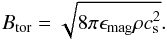 (15)In the initial condition, the ratio of the magnetic to thermal pressure will in particular influence the scale height of the disk, the gas distribution, and the rotational velocity.
 |
Fig. 1 Density slice in the x − y plane at different times showing the global evolution in the simulation box (run A), including the merger stage at about 4 Gyr and the post-merger configuration after 5 Gyr. |
2.4. Simulation box
Overall, we considered a cubic simulation box of size 500 kpc with periodic boundary conditions, containing two idealized disks of equal mass 0.5 × 10¹¹M⊙ that are aligned with the x − y plane. They have a scale radius of 10 kpc and a separation of 150 kpc, aligned with the y-axis. For the intergalactic medium, we adopted a mean density of ~7 × 10-30 g cm-3. The gas in the disks and in the intergalactic medium was assumed to be isothermal at a temperature of 5 × 10⁴ K. We adopted a ratio of magnetic to thermal pressure of ϵmag = 0.5. The magnetic field in the intergalactic medium was randomly orientated, with an rms value of 10-25 G. The medium outside the galaxies was thus strongly dominated by the thermal pressure. Potential divergences of the magnetic field were thus of low magnitude and taken care of by divergence cleaning.
The relative velocity of the galaxies is initially aligned with the x-direction and corresponds to 20 km s-1 (each galaxy moving with half of that velocity in opposite directions). The velocity was chosen here for practical purposes because higher initial velocities require a considerably larger simulation box.
To resolve the initial structures and their subsequent evolution, we employed the adaptive mesh-refinement technique, with a top grid resolution of 323 and six additional refinement levels, each increasing the resolution by a factor of 2. The latter corresponds to an effective resolution of 0.24 pc in the simulation. A new refinement level was introduced in the initial condition and during the dynamical evolution whenever the Jeans length was resolved by fewer than 32 cells, so that the internal disk structure was well resolved. The simulation was evolved for 10 Gyr to follow the dynamical evolution.
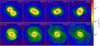 |
Fig. 2 Gas density projections between 3.25 Gyr and 5.6 Gyr, showing the evolution on scales of 250 kpc around the merger event (run A). The galaxy cores are clearly merged at a time of 4.4 Gyr. |
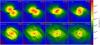 |
Fig. 3 Density-weighted projections of the magnetic energy density between 3.25 Gyr and 5.6 Gyr, showing the evolution on scales of 250 kpc around the merger event (run A). The structure visible in the magnetic energy resembles the structure visible in the gas density. The galaxy cores have clearly merged after 4.4 Gyr. We indicate the region over which the field strength of the whole galaxy is averaged with circles (25 kpc), and also the region corresponding to an average over the center (5 kpc). The circles are centered on the density peak in the simulation. |
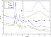 |
Fig. 4 Evolution of the average magnetic field strength within the central 5 kpc, within the central 25 kpc, and on the scales between 5 and 25 kpc as a function of time (run A). |
3. Results
In the following, we first describe our reference run in greater detail to show the main qualitative features that may occur. In particular, we demonstrate from the reference run that geometric effects are sufficient to explain the qualitative behavior that has been observed. Subsequently, we show additional runs with varying parameters to address possible variations that may occur. A list of all simulations presented here is given in Table 1; the reference run corresponds to run A in the list.
List of simulations presented here.
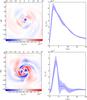 |
Fig. 5 Magnetic field structure before the merger (at 3 Gyr) and after the merger (at 5 Gyr, i.e., about 0.6 Gyr after the merger of the core). Left: projection of the fluctuation of the toroidal magnetic field strength (local toroidal field minus mean toroidal field at the same radius) in the central 40 kpc. Right: radial profile of the toroidal magnetic field as a function of radius, including its rms distribution. Both plots refer to the reference run A. |
3.1. Reference run
The global evolution in our simulation box is shown in Fig. 1 using density slices in the x − y plane. The isolated disks initially move in opposite directions along the x-axis, but start approaching each other along the y-direction as a result of their gravitational interaction. After 1 Gyr, the low-density gas (~10-27 g cm-3) at the very outskirts of the galaxies starts to interact, which leads to the development of shocks. The interactions become more intense while the cores of the disks are approaching each other. After 4 Gyr, the interaction extends to higher-density gas components (~10-25 g cm-3), which leads to the formation of a disk around the galaxy cores, including signs of self-gravitational instabilities. The cores are clearly merged after 5 Gyr, and the disk surrounding the central core shows spiral arm features characteristic of self-gravitating disks.
The evolution closer to the merger event is presented in Fig. 2, showing density projections at different times between 3.25 Gyr and 5.6 Gyr. At 3.25 Gyr, the cores of the disks are still separated, while the surrounding gas starts to merge and forms a joint structure surrounding the cores. At 3.75 Gyr, the cores have reached a separation of less than 10 kpc. When reaching this separation, the cores still possess a significant amount of kinetic energy, however, so that the separation increases again toward ~4 Gyr. The overall process is strongly damped by the hydrodynamical interaction, however, and the cores fast approach each other again at 4.4 Gyr, leading to the final merger event. At 3.75 − 4 Gyr, the gas surrounding the cores shows bar-like features and signs of strong gravitational instability, which develops into spiral arm features after the merger.
The corresponding evolution of the magnetic energy density is given in Fig. 3. This evolution is closely related to the evolution of the density structure. For a comparison with observational data, in particular the merger sequence compiled by Drzazga et al. (2011), we calculated the magnetic field strength averaged over different scales during the evolution of the merger. In particular, we determined the average field strength within 5 kpc, within 25 kpc, and in the region between 5 and 25 kpc. These regions can be roughly associated with the magnetic field strengths provided by Drzazga et al. (2011), who considered the average magnetic field strength in the galaxy center (~6.5 kpc), in the whole galaxy, and in the outer parts of the galaxy. The regions employed for the averaging procedure are denoted with circles in Fig. 3, and the evolution of the resulting magnetic field strengths as a function of time is given in Fig. 4. The circles are centered onto the density peaks of the simulation. Especially for two disks with equal mass, the position of the peak may then jump from one disk to another. As the situation is highly symmetric, the latter is irrelevant for the determination of the averaged magnetic field strength on the different scales, however, giving rise to a rather smooth evolution, as shown in Fig. 4. For disks with unequal mass, we have checked that the density peak remains on the disk with the higher mass.
For the magnetic field averages on all three scales explored here, clear peaks can be recognized at about 3.75 Gyr and ~4.4 Gyr. While the peak at 4.4 Gyr corresponds to the merger of the galaxy cores, the cores are still clearly separated at ~3.75 Gyr. The latter can be understood from a comparison with Fig. 3. At a time of 3.75 Gyr, the galaxy cores are still separated, but close enough that both galaxy cores fall into the characteristic scale of 25 kpc. This naturally explains the peak in the field strength averaged over the entire galaxy, as an additional strong contribution from the second core is included in the average. Similarly, this core will also contribute to the magnetic field strength in the outer region, corresponding to distances between 5 and 25 kpc from the center of the first core. In addition, however, the magnetic field strength within the central 5 kpc is also enhanced by a similar factor. As the cores are still clearly separated, the latter is not due to a geometric effect. Instead, as a result of the tidal torques resulting from the presence of the additional core, the angular momentum transport within the galaxy is enhanced, increasing the density and the magnetic field strength within the central region, explaining the peak in the central region of the disk. This is also consistent with the density evolution found in Fig. 2.
For the peak at 4.4 Gyr, both cores are again within the radius of 25 kpc, explaining the enhancement on the scale of the galaxy and in its outer regions. During that time, moreover, the two cores actually merge, providing again a physical enhancement of the magnetic field strength on scales of ~5 kpc. We note that the second peak is smaller than the first. This is at least partly due to the fact that the gas in the galaxy, which has come very close during the merger event, again begins to encompass a somewhat larger surface area because not all the kinetic energy has been dissipated by the shocks, and some of it now leads to the formation of a more well-defined disk as the result of angular momentum. The latter also leads to a redistribution of the magnetic energy.
While the magnetic field strength before the merger is well aligned with the rotation of the galaxy and predominantly has a toroidal component, the latter changes significantly as a consequence of the merger event. In Fig. 5 we show on the left-hand side the fluctuation of the toroidal magnetic field component, defined as its local value at a given position minus the mean toroidal field strength at the same radius, in a projection of the central 40 kpcat 3 Gyr well before the merger and at a time of 5 Gyr, that is, about 0.6 Gyr after the merger of the central cores. At 3 Gyr, the initial profile of the magnetic field strength (resulting from equipartition with a fixed fraction ϵmag of the thermal energy) is still mostly intact, and fluctuations in the toroidal component are generally weak. After the merger, the radial profile of the toroidal field is strongly disrupted and influenced by the presence of spiral arms, and the scatter in the toroidal component is significantly enhanced, with an rms deviation that is comparable to the mean.
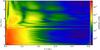 |
Fig. 6 Power spectrum of the magnetic field in the simulation box as a sequence of time (run A). While the magnetic energy is initially localized on larger scales owing to the coherent toroidal field, a distinct peak at 3.6 Gyr and ~4.4 Gyr is visible. This is due to the generation of fluctuations on smaller scales, in particular through the decreasing separation of the central cores. While these peaks disappear again after the merger, a noticeable amount of power is nevertheless shifted to smaller scales. |
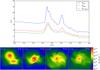 |
Fig. 7 Comparison run with a relative disk orientation of 90° (run B). Top: time evolution of the mean magnetic field strength on different scales. Bottom: projection of the magnetic pressure at different times. |
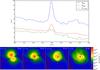 |
Fig. 8 Comparison run with a mass ratio of 1:3 (run C). Top: time evolution of the mean magnetic field strength on different scales. Bottom: projection of the magnetic pressure at different times. |
The latter is examined in Fig. 6 in more detail, where we show the power spectrum of the magnetic field in our simulation as a time sequence. Two peaks at 3.75 Gyr and 4.4 Gyr are evident, reflecting the additional power on small scales during the merger. While these peaks disappear after the merger, a considerable amount of power has shifted to a smaller scale. In addition, the overall power in the field strength decreases after the merger, reflecting the behavior that is also found for the average strength of the magnetic field. The latter is due to a slight expansion of the disk that we observe in all simulations after the merger, thus causing a spread in the mass and the magnetic energy over a larger volume. We expect that an external potential provided by a stellar and dark matter component would help to stabilize the size of the gaseous disks. Even in this case, a relaxation of the disk after the merger would be expected because of the release of gravitational energy, however.
3.2. Parameter variations
To at least qualitatively understand how the results shown here depend on the adopted configuration, we varied the choice of the orbit, the relative disk orientation, and the merger mass ratio. As a first interesting case, we present a simulation in Fig. 7 with a relative disk orientation of 90° (run B). In this case, the global dynamics before the merger event change only to a minor degree. In particular, there are still two events where both disks fit into the beam, showing an apparent amplification in an average over galactic scales.
To explore the effect of varying the mass ratio while keeping our focus on major mergers, that is, neglecting minor events that can be considered as small perturbations of the main galaxy, we also show a simulation with mass ratio 3:1 in Fig. 8 run C), where the mass of the more massive disk is unchanged. This changes the dynamics sufficiently to lead to a more rapid merger event. As a result, the disks merge directly after the first encounter, providing only one peak in the large-scale averaged magnetic field strength, and without orbiting the larger galaxy another time.
To explore changes in the orbit, we also present two simulations where we changed the relative initial velocity, as shown in Fig. 9. These cases correspond to initial relative velocities of 10 km s-1 (run D) and 15 km s-1 (run E), respectively. In both cases, the merger of the disks significantly accelerates, and we see essentially one peak in the time evolution of the average magnetic field strength. The bottom panel of the figure, corresponding to the relative velocity of 15 km s-1, still shows a minor hint of a potential second peak, as a result of an incomplete initial merging process. We note, however, that this feature is not comparable in size to what we see in our reference run.
While of course the sample of configurations adopted here is still limited, the occurrence of one or two peaksin the magnetic field strength evolution as a result of geometric projection events is a generic phenomenon we can infer from these simulations. The implications of these results should thus be considered in the interpretation of data from larger beams. As a possible way to consider the geometric projection effects described here, we suggest to normalize the inferred strength of the magnetic field with respect to the size of the gaseous component, providing a better measure of the magnetic field strength in the galaxy rather independently from the size of the magnetized region.
4. Discussion and conclusions
To explore the evolution of magnetic fields during merger events, we presented a toy model for simulating the evolution of magnetic fields during the mergers. For this purpose, we modeled the interaction of two gaseous magnetized disks to explore how the interaction of the gas changes the structure of the magnetic field. In these idealized simulations, we neglected the presence of a stellar component and a dark matter halo. While the neglect of the dark matter halo can certainly have an effect on the orbit and change the dynamics, we also showed in our sample of simulations that a set of characteristic features is rather insensitive to the details of the orbit. We describe below in more detail how part of the results may change after the inclusion of dark matter halos.
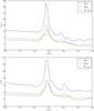 |
Fig. 9 Comparison runs with a lower relative velocity between the disks. We focus here on the time evolution of the magnetic field strength averaged over different length scales. Top: relative velocity of 10 km s-1 (run D). Bottom: relative velocity of 15 km s-1 (run E). |
In spite of the simplicity of our model, we were able to reproduce central characteristics of the magnetic field evolution in the merger sequence provided by Drzazga et al. (2011). In particular, they have shown a characteristic peak in the average field strength of the galaxy, its central regions, and also in the outer parts of the galaxy when plotted against the interaction parameter. For comparison, we followed the time evolution of the magnetic field in the central 5 kpc of the galaxy, within a 25 kpc radius, and in the region between 5 kpc and 25 kpc. We expect the latter to approximately resemble the three cases distinguished by Drzazga et al. (2011). In our reference run, we found two characteristic peaks in these quantities during the merger event. The peak in the average field strength within the galaxy and its outer region can be naturally explained by geometrical effects when the core of the second disk falls into the region covered by the 25 kpc radius. Within the central 5 kpc, the magnetic field strength and the central density are enhanced as a result of the increased angular momentum transport induced by the tidal torques within the configuration. The first peak occurs when the two cores for the first time come very close, but do not merge, while the second peak occurs when the two cores are about to merge. We note, however, that the occurrence of two peaks is not critical, and one peak in the averaged field strength, as observed in other simulations, is enough to explain the sequence derived by Drzazga et al. (2011).
Despite their simplifications, our simulations can thus naturally explain the occurrence of a peak in the magnetic field strength during the merger. We note that the time sequence produced in the simulation may not correspond one to one to the merger sequence produced by Drzazga et al. (2011), and in particular the interaction parameter may not uniquely correspond to a single time in the simulation, but rather to the characteristic times when the central cores come very close. Concerning the physical interpretation, our results show that there is a clear distinction between geometrical effects on the one hand, as the average field strength will increase when the core of one galaxy enters the outer parts of another one, and physical changes in the magnetic field strength in particular in the center of the galaxy on the other hand, either caused by density enhancements or possibly by dynamo effects. High-resolution observations to explore the central regions of merging galaxies are therefore particularly valuable to further explore the increase in the magnetic field strength during the merger along with its physical origin.
We have checked that the results presented here do not strongly depend on the parameters in the simulations, such as the mass of the galaxy, their relative velocity, or the initial magnetic field strength. In some cases, we found the emergence of only one peak insted of two, depending on the detailed evolution of the final merger. This behavior tends to occur when the relative velocities are lower between the galaxies, leading to a more rapid merger event. In this case, there will be only one event where both disks fall into the observed beam, leading to two contributions. This also confirms that geometrical effects play the dominant role in case of large beams, and only high-resolution observations can help to assess the physical behavior of the magnetic fields.
For realistic simulations, a dark matter halo should be included for both galaxies. To zero order, the latter will enhance the gravitational and the inertial mass. While the baryons in the disks interacted strongly, which led to a relevant amount of friction, the latter will be reduced for the mass in dark matter. However, we note that even the dark matter halos will experience dynamical friction while moving through the circumgalactic material, including baryonic and dark matter. While a precise orbit can only be obtained through dedicated simulations for each specific configuration, we expect that overall friction effects will be less relevant in a dark matter dominated regime, suggesting that the final merger may be somewhat delayed. The latter may affect the overall probability to find a specific galaxy in a certain merger stage, while the resulting geometrical projection effects are most likely the same.
As we noted in the introduction, previous investigations concerning the evolution of magnetic fields during galaxy mergers have predominantly been pursued using MHD-SPH simulations (e.g., Kotarba et al. 2010, 2011; Geng et al. 2012), or in the 2D approximation using a grid-based approach (Moss et al. 2014). Even the number of studies of isolated galaxies including magnetic fields is still limited. In this respect, we note the simulations pursued by Wang & Abel (2009) to explore galaxy formation in a cosmological context, where they neglected stellar feedback. More recently, Pakmor & Springel (2013) pursued simulations of isolated disk galaxies including magnetic fields and stellar feedback using a moving-mesh approach. Magnetic field amplification in isolated galaxies has also been explored in the 2D approximation (Moss et al. 2015) or by simulating local volumes (Gressel et al. 2008). The interaction of the dynamo process with cosmic rays has furthermore been explored by Hanasz et al. (2009). Hydrodynamical simulations of isolated galaxies have been pursued with the Enzo code by (e.g. Tasker & Tan 2009), and gravitational instabilities in isolated disks have been explored by Lichtenberg & Schleicher (2015).
While we have shown here that even simplified models can reproduce some of the main features in the observed merger sequence, future simulations should aim for a more detailed and more realistic modeling, accounting for the effects of feedback, and employing cosmological initial conditions. In the context of isolated disk galaxies, the latter has been achieved by Wang & Abel (2009), Latif et al. (2014), and Pakmor et al. (2014), but it is yet to be achieved in the context of galaxy mergers. An additional problem is the limited resolution in numerical simulations, implying that galaxy-scale simulations will never be able to resolve turbulence and small-scale magnetic fields on all relevant scales. In the MHD equations, it may therefore be necessary to adopt nonlinear closures to explore the resulting dynamical implications (Grete et al. 2015, 2016; Vlaykov et al. 2016). The latter was shown to be relevant in hydrodynamical simulations of isolated galaxies (e.g., Braun et al. 2014; Braun & Schmidt 2015), and we expect similar effects to occur in MHD simulations.
Webpage Enzo: http://enzo-project.org/
Acknowledgments
We acknowledge fruitful discussions with Muhammad Latif concerning the MHD implementation in Enzo. The simulation results are analyzed using the visualization toolkit for astrophysical data YT (Turk et al. 2011). K.R. acknowledges financial support by the International Max Planck Research School for Solar System Science at the University of Göttingen. D.R.G.S. thanks for funding through Fondecyt regular (project code 1161247) and through the “Concurso Proyectos Internacionales de Investigación, Convocatoria 2015” (project code PII20150171).
References
- Banerjee, R., Vázquez-Semadeni, E., Hennebelle, P., & Klessen, R. S. 2009, MNRAS, 398, 1082 [NASA ADS] [CrossRef] [Google Scholar]
- Barnes, J. E. 1988, ApJ, 331, 699 [NASA ADS] [CrossRef] [Google Scholar]
- Barnes, J. E. 1992, ApJ, 393, 484 [NASA ADS] [CrossRef] [Google Scholar]
- Basu, A., Roy, S., & Mitra, D. 2012, ApJ, 756, 141 [NASA ADS] [CrossRef] [Google Scholar]
- Beck, R., Ehle, M., Shoutenkov, V., Shukurov, A., & Sokoloff, D. 1999, Nature, 397, 324 [NASA ADS] [CrossRef] [Google Scholar]
- Beck, R., Fletcher, A., Shukurov, A., et al. 2005, A&A, 444, 739 [NASA ADS] [CrossRef] [EDP Sciences] [Google Scholar]
- Bhat, P., & Subramanian, K. 2014, ApJ, 791, L34 [NASA ADS] [CrossRef] [Google Scholar]
- Bourne, N., Dunne, L., Ivison, R. J., et al. 2011, MNRAS, 410, 1155 [NASA ADS] [CrossRef] [Google Scholar]
- Brandenburg, A., & Subramanian, K. 2005, Phys. Rep., 417, 1 [NASA ADS] [CrossRef] [Google Scholar]
- Brassington, N. J., Ponman, T. J., & Read, A. M. 2007, MNRAS, 377, 1439 [NASA ADS] [CrossRef] [Google Scholar]
- Braun, H., & Schmidt, W. 2015, MNRAS, 454, 1545 [NASA ADS] [CrossRef] [Google Scholar]
- Braun, H., Schmidt, W., Niemeyer, J. C., & Almgren, A. S. 2014, MNRAS, 442, 3407 [NASA ADS] [CrossRef] [Google Scholar]
- Bryan, G. L., Norman, M. L., O’Shea, B. W., et al. 2014, ApJS, 211, 19 [NASA ADS] [CrossRef] [Google Scholar]
- Capelo, P. R., Volonteri, M., Dotti, M., et al. 2015, MNRAS, 447, 2123 [NASA ADS] [CrossRef] [Google Scholar]
- Casey, C. M., Berta, S., Béthermin, M., et al. 2012, ApJ, 761, 140 [NASA ADS] [CrossRef] [Google Scholar]
- Cho, J., Vishniac, E. T., Beresnyak, A., Lazarian, A., & Ryu, D. 2009, ApJ, 693, 1449 [NASA ADS] [CrossRef] [Google Scholar]
- Chyży, K. T., & Beck, R. 2004, A&A, 417, 541 [NASA ADS] [CrossRef] [EDP Sciences] [Google Scholar]
- Chyży, K. T., Beck, R., Kohle, S., Klein, U., & Urbanik, M. 2000, A&A, 355, 128 [NASA ADS] [Google Scholar]
- Chyży, K. T., Weżgowiec, M., Beck, R., & Bomans, D. J. 2011, A&A, 529, A94 [NASA ADS] [CrossRef] [EDP Sciences] [Google Scholar]
- Collins, D. C., Xu, H., Norman, M. L., Li, H., & Li, S. 2010, ApJS, 186, 308 [NASA ADS] [CrossRef] [Google Scholar]
- Condon, J. J. 1983, ApJS, 53, 459 [NASA ADS] [CrossRef] [Google Scholar]
- Condon, J. J., Helou, G., Sanders, D. B., & Soifer, B. T. 1993, AJ, 105, 1730 [Google Scholar]
- Condon, J. J., Helou, G., & Jarrett, T. H. 2002, AJ, 123, 1881 [Google Scholar]
- de Jong, T., Klein, U., Wielebinski, R., & Wunderlich, E. 1985, A&A, 147, L6 [NASA ADS] [Google Scholar]
- Dedner, A., Kemm, F., Kröner, D., et al. 2002, J. Comput. Phys., 175, 645 [Google Scholar]
- Drzazga, R. T., Chyży, K. T., Jurusik, W., & Wiórkiewicz, K. 2011, A&A, 533, A22 [NASA ADS] [CrossRef] [EDP Sciences] [Google Scholar]
- Elmegreen, B. G., Sundin, M., Kaufman, M., Brinks, E., & Elmegreen, D. M. 1995a, ApJ, 453, 139 [NASA ADS] [CrossRef] [Google Scholar]
- Elmegreen, D. M., Kaufman, M., Brinks, E., Elmegreen, B. G., & Sundin, M. 1995b, ApJ, 453, 100 [NASA ADS] [CrossRef] [Google Scholar]
- Fabbiano, G., Zezas, A., & Murray, S. S. 2001, ApJ, 554, 1035 [NASA ADS] [CrossRef] [Google Scholar]
- Federrath, C., & Klessen, R. S. 2012, ApJ, 761, 156 [NASA ADS] [CrossRef] [Google Scholar]
- Federrath, C., Chabrier, G., Schober, J., et al. 2011, Phys. Rev. Lett., 107, 114504 [NASA ADS] [CrossRef] [Google Scholar]
- Ferrara, A., Haardt, F., & Salvaterra, R. 2013, MNRAS, 434, 2600 [NASA ADS] [CrossRef] [Google Scholar]
- Fletcher, A., Beck, R., Shukurov, A., Berkhuijsen, E. M., & Horellou, C. 2011, MNRAS, 412, 2396 [NASA ADS] [CrossRef] [MathSciNet] [Google Scholar]
- Forbes, D. A., Ponman, T. J., & Brown, R. J. N. 1998, ApJ, 508, L43 [NASA ADS] [CrossRef] [Google Scholar]
- Freeman, K. C. 1970, ApJ, 160, 811 [NASA ADS] [CrossRef] [Google Scholar]
- Gallimore, J. F., & Keel, W. C. 1993, AJ, 106, 1337 [NASA ADS] [CrossRef] [Google Scholar]
- Gao, Y., & Solomon, P. M. 1999, ApJ, 512, L99 [NASA ADS] [CrossRef] [Google Scholar]
- Gao, Y., Zhu, M., & Seaquist, E. R. 2003, AJ, 126, 2171 [NASA ADS] [CrossRef] [Google Scholar]
- Geng, A., Kotarba, H., Bürzle, F., et al. 2012, MNRAS, 419, 3571 [NASA ADS] [CrossRef] [Google Scholar]
- Georgakakis, A., Forbes, D. A., & Norris, R. P. 2000, MNRAS, 318, 124 [NASA ADS] [CrossRef] [Google Scholar]
- Gressel, O., Elstner, D., Ziegler, U., & Rüdiger, G. 2008, A&A, 486, L35 [NASA ADS] [CrossRef] [EDP Sciences] [Google Scholar]
- Gressel, O., Bendre, A., & Elstner, D. 2013, MNRAS, 429, 967 [NASA ADS] [CrossRef] [Google Scholar]
- Grete, P., Vlaykov, D. G., Schmidt, W., Schleicher, D. R. G., & Federrath, C. 2015, New J. Phys., 17, 023070 [NASA ADS] [CrossRef] [Google Scholar]
- Grete, P., Vlaykov, D. G., Schmidt, W., & Schleicher, D. R. G. 2016, Phys. Plasmas, 23, 062317 [NASA ADS] [CrossRef] [Google Scholar]
- Hanasz, M., Wóltański, D., & Kowalik, K. 2009, ApJ, 706, L155 [NASA ADS] [CrossRef] [Google Scholar]
- Heesen, V., Rau, U., Rupen, M. P., Brinks, E., & Hunter, D. A. 2011, ApJ, 739, L23 [NASA ADS] [CrossRef] [Google Scholar]
- Heesen, V., Brinks, E., Leroy, A. K., et al. 2014, AJ, 147, 103 [NASA ADS] [CrossRef] [Google Scholar]
- Helou, G., Soifer, B. T., & Rowan-Robinson, M. 1985, ApJ, 298, L7 [Google Scholar]
- Hernquist, L. 1992, ApJ, 400, 460 [NASA ADS] [CrossRef] [Google Scholar]
- Hernquist, L. 1993, ApJ, 409, 548 [NASA ADS] [CrossRef] [Google Scholar]
- Hibbard, J. E., & van Gorkom, J. H. 1996, AJ, 111, 655 [NASA ADS] [CrossRef] [Google Scholar]
- Hummel, E. 1981, A&A, 96, 111 [NASA ADS] [Google Scholar]
- Hummel, E., van der Hulst, J. M., Kennicutt, R. C., & Keel, W. C. 1990, A&A, 236, 333 [NASA ADS] [Google Scholar]
- Ivison, R. J., Magenelli, B., Ibar, E., et. al. 2010, A&A, 518, L31 [NASA ADS] [CrossRef] [EDP Sciences] [Google Scholar]
- Jarvis, M. J., Smith, D. J. B., Bonfield, D. G., et al. 2010, MNRAS, 409, 92 [NASA ADS] [CrossRef] [Google Scholar]
- Joseph, R. D., & Wright, G. S. 1985, MNRAS, 214, 87 [NASA ADS] [Google Scholar]
- Keel, W. C., & Wu, W. 1995, AJ, 110, 129 [NASA ADS] [CrossRef] [Google Scholar]
- Keel, W. C., Kennicutt, Jr., R. C., Hummel, E., & van der Hulst, J. M. 1985, AJ, 90, 708 [NASA ADS] [CrossRef] [Google Scholar]
- Kennicutt, Jr., R. C. 1998, ARA&A, 36, 189 [Google Scholar]
- Kepley, A. A., Mühle, S., Everett, J., et al. 2010, ApJ, 712, 536 [NASA ADS] [CrossRef] [Google Scholar]
- Kepley, A. A., Zweibel, E. G., Wilcots, E. M., Johnson, K. E., & Robishaw, T. 2011, ApJ, 736, 139 [NASA ADS] [CrossRef] [Google Scholar]
- Klaas, U., Nielbock, M., Haas, M., Krause, O., & Schreiber, J. 2010, A&A, 518, L44 [NASA ADS] [CrossRef] [EDP Sciences] [Google Scholar]
- Kotarba, H., Karl, S. J., Naab, T., et al. 2010, ApJ, 716, 1438 [NASA ADS] [CrossRef] [Google Scholar]
- Kotarba, H., Lesch, H., Dolag, K., et al. 2011, MNRAS, 415, 3189 [NASA ADS] [CrossRef] [Google Scholar]
- Latif, M. A., Schleicher, D. R. G., & Schmidt, W. 2014, MNRAS, 440, 1551 [NASA ADS] [CrossRef] [Google Scholar]
- Lawrence, A., Rowan-Robinson, M., Leech, K., Jones, D. H. P., & Wall, J. V. 1989, MNRAS, 240, 329 [NASA ADS] [Google Scholar]
- Lichtenberg, T., & Schleicher, D. R. G. 2015, A&A, 579, A32 [NASA ADS] [CrossRef] [EDP Sciences] [Google Scholar]
- Malin, D. F., & Carter, D. 1980, Nature, 285, 643 [NASA ADS] [CrossRef] [Google Scholar]
- Mayer, L., Kazantzidis, S., Escala, A., & Callegari, S. 2010, Nature, 466, 1082 [NASA ADS] [CrossRef] [Google Scholar]
- Mihos, J. C., & Hernquist, L. 1996, ApJ, 464, 641 [NASA ADS] [CrossRef] [Google Scholar]
- Moss, D., Sokoloff, D., Beck, R., & Krause, M. 2014, A&A, 566, A40 [NASA ADS] [CrossRef] [EDP Sciences] [Google Scholar]
- Moss, D., Stepanov, R., Krause, M., Beck, R., & Sokoloff, D. 2015, A&A, 578, A94 [NASA ADS] [CrossRef] [EDP Sciences] [Google Scholar]
- Murphy, E. J. 2009, ApJ, 706, 482 [NASA ADS] [CrossRef] [Google Scholar]
- Niklas, S., & Beck, R. 1997, A&A, 320, 54 [NASA ADS] [Google Scholar]
- O’Shea, B. W., Bryan, G., Bordner, J., et al. 2004 [arXiv:astro-ph/0403044] [Google Scholar]
- Pakmor, R., & Springel, V. 2013, MNRAS, 432, 176 [NASA ADS] [CrossRef] [Google Scholar]
- Pakmor, R., Marinacci, F., & Springel, V. 2014, ApJ, 783, L20 [NASA ADS] [CrossRef] [Google Scholar]
- Park, K., Blackman, E. G., & Subramanian, K. 2013, Phys. Rev. E, 87, 053110 [NASA ADS] [CrossRef] [Google Scholar]
- Planesas, P., Colina, L., & Perez-Olea, D. 1997, A&A, 325, 81 [NASA ADS] [Google Scholar]
- Privon, G. C., Barnes, J. E., Evans, A. S., et al. 2013, ApJ, 771, 120 [NASA ADS] [CrossRef] [Google Scholar]
- Read, A. M., & Ponman, T. J. 1998, MNRAS, 297, 143 [NASA ADS] [CrossRef] [Google Scholar]
- Rossa, J., Laine, S., van der Marel, R. P., et al. 2007, AJ, 134, 2124 [NASA ADS] [CrossRef] [Google Scholar]
- Ruediger, G., & Kichatinov, L. L. 1993, A&A, 269, 581 [NASA ADS] [Google Scholar]
- Sanders, D. B., & Mirabel, I. F. 1996, ARA&A, 34, 749 [NASA ADS] [CrossRef] [Google Scholar]
- Schekochihin, A. A., Cowley, S. C., Hammett, G. W., Maron, J. L., & McWilliams, J. C. 2002, New J. Phys., 4, 84 [NASA ADS] [CrossRef] [Google Scholar]
- Schleicher, D. R. G., & Beck, R. 2013, A&A, 556, A142 [NASA ADS] [CrossRef] [EDP Sciences] [Google Scholar]
- Schleicher, D. R. G., & Beck, R. 2016, A&A, 593, A77 [NASA ADS] [CrossRef] [EDP Sciences] [Google Scholar]
- Schleicher, D. R. G., Schober, J., Federrath, C., Bovino, S., & Schmidt, W. 2013, New J. Phys., 15, 023017 [NASA ADS] [CrossRef] [Google Scholar]
- Schober, J., Schleicher, D., Federrath, C., Klessen, R., & Banerjee, R. 2012, Phys. Rev. E, 85, 026303 [NASA ADS] [CrossRef] [Google Scholar]
- Schober, J., Schleicher, D. R. G., Federrath, C., Bovino, S., & Klessen, R. S. 2015, Phys. Rev. E, 92, 023010 [NASA ADS] [CrossRef] [Google Scholar]
- Schober, J., Schleicher, D. R. G., & Klessen, R. S. 2016, ApJ, 827, 109 [NASA ADS] [CrossRef] [Google Scholar]
- Schweizer, F., & Seitzer, P. 1988, ApJ, 328, 88 [NASA ADS] [CrossRef] [Google Scholar]
- Smith, B. J., Giroux, M. L., Struck, C., & Hancock, M. 2010, AJ, 139, 1212 [NASA ADS] [CrossRef] [Google Scholar]
- Soifer, B. T., Sanders, D. B., Madore, B. F., et al. 1987, ApJ, 320, 238 [NASA ADS] [CrossRef] [Google Scholar]
- Surace, J. A., Mazzarella, J., Soifer, B. T., & Wehrle, A. E. 1993, AJ, 105, 864 [NASA ADS] [CrossRef] [Google Scholar]
- Tabatabaei, F. S., Berkhuijsen, E. M., Frick, P., Beck, R., & Schinnerer, E. 2013, A&A, 557, A129 [NASA ADS] [CrossRef] [EDP Sciences] [Google Scholar]
- Tasker, E. J., & Tan, J. C. 2009, ApJ, 700, 358 [NASA ADS] [CrossRef] [Google Scholar]
- Toomre, A. 1977, in Evolution of Galaxies and Stellar Populations, eds. B. M. Tinsley, R. B. G. Larson, & D. Campbell, 401 [Google Scholar]
- Treister, E., Schawinski, K., Urry, C. M., & Simmons, B. D. 2012, ApJ, 758, L39 [NASA ADS] [CrossRef] [Google Scholar]
- Turk, M. J., Smith, B. D., Oishi, J. S., et al. 2011, ApJS, 192, 9 [NASA ADS] [CrossRef] [Google Scholar]
- Ueda, J., Iono, D., Petitpas, G., et al. 2012, ApJ, 745, 65 [NASA ADS] [CrossRef] [Google Scholar]
- van Leer, B. 1979, J. Comput. Phys., 32, 101 [Google Scholar]
- Vázquez-Semadeni, E., Banerjee, R., Gómez, G. C., et al. 2011, MNRAS, 414, 2511 [NASA ADS] [CrossRef] [Google Scholar]
- Vlaykov, D. G., Grete, P., Schmidt, W., & Schleicher, D. R. 2016, Phys. Plasmas, 23, 062316 [NASA ADS] [CrossRef] [Google Scholar]
- Wang, P., & Abel, T. 2009, ApJ, 696, 96 [NASA ADS] [CrossRef] [Google Scholar]
- Wang, H.-H., Klessen, R. S., Dullemond, C. P., van den Bosch, F. C., & Fuchs, B. 2010, MNRAS, 407, 705 [NASA ADS] [CrossRef] [Google Scholar]
- Yun, M. S., Reddy, N. A., & Condon, J. J. 2001, ApJ, 554, 803 [NASA ADS] [CrossRef] [Google Scholar]
- Zhu, M., Gao, Y., Seaquist, E. R., & Dunne, L. 2007, AJ, 134, 118 [NASA ADS] [CrossRef] [Google Scholar]
All Tables
All Figures
|
Fig. 1 Density slice in the x − y plane at different times showing the global evolution in the simulation box (run A), including the merger stage at about 4 Gyr and the post-merger configuration after 5 Gyr. |
| In the text | |
|
Fig. 2 Gas density projections between 3.25 Gyr and 5.6 Gyr, showing the evolution on scales of 250 kpc around the merger event (run A). The galaxy cores are clearly merged at a time of 4.4 Gyr. |
| In the text | |
|
Fig. 3 Density-weighted projections of the magnetic energy density between 3.25 Gyr and 5.6 Gyr, showing the evolution on scales of 250 kpc around the merger event (run A). The structure visible in the magnetic energy resembles the structure visible in the gas density. The galaxy cores have clearly merged after 4.4 Gyr. We indicate the region over which the field strength of the whole galaxy is averaged with circles (25 kpc), and also the region corresponding to an average over the center (5 kpc). The circles are centered on the density peak in the simulation. |
| In the text | |
|
Fig. 4 Evolution of the average magnetic field strength within the central 5 kpc, within the central 25 kpc, and on the scales between 5 and 25 kpc as a function of time (run A). |
| In the text | |
|
Fig. 5 Magnetic field structure before the merger (at 3 Gyr) and after the merger (at 5 Gyr, i.e., about 0.6 Gyr after the merger of the core). Left: projection of the fluctuation of the toroidal magnetic field strength (local toroidal field minus mean toroidal field at the same radius) in the central 40 kpc. Right: radial profile of the toroidal magnetic field as a function of radius, including its rms distribution. Both plots refer to the reference run A. |
| In the text | |
|
Fig. 6 Power spectrum of the magnetic field in the simulation box as a sequence of time (run A). While the magnetic energy is initially localized on larger scales owing to the coherent toroidal field, a distinct peak at 3.6 Gyr and ~4.4 Gyr is visible. This is due to the generation of fluctuations on smaller scales, in particular through the decreasing separation of the central cores. While these peaks disappear again after the merger, a noticeable amount of power is nevertheless shifted to smaller scales. |
| In the text | |
|
Fig. 7 Comparison run with a relative disk orientation of 90° (run B). Top: time evolution of the mean magnetic field strength on different scales. Bottom: projection of the magnetic pressure at different times. |
| In the text | |
|
Fig. 8 Comparison run with a mass ratio of 1:3 (run C). Top: time evolution of the mean magnetic field strength on different scales. Bottom: projection of the magnetic pressure at different times. |
| In the text | |
|
Fig. 9 Comparison runs with a lower relative velocity between the disks. We focus here on the time evolution of the magnetic field strength averaged over different length scales. Top: relative velocity of 10 km s-1 (run D). Bottom: relative velocity of 15 km s-1 (run E). |
| In the text | |
Current usage metrics show cumulative count of Article Views (full-text article views including HTML views, PDF and ePub downloads, according to the available data) and Abstracts Views on Vision4Press platform.
Data correspond to usage on the plateform after 2015. The current usage metrics is available 48-96 hours after online publication and is updated daily on week days.
Initial download of the metrics may take a while.