| Issue |
A&A
Volume 592, August 2016
|
|
|---|---|---|
| Article Number | A14 | |
| Number of page(s) | 27 | |
| Section | Stellar structure and evolution | |
| DOI | https://doi.org/10.1051/0004-6361/201527987 | |
| Published online | 05 July 2016 | |
SpaceInn hare-and-hounds exercise: Estimation of stellar properties using space-based asteroseismic data
1 School of Physics and Astronomy, University of Birmingham, Edgbaston, Birmingham B15 2TT, UK
2 Stellar Astrophysics Centre (SAC), Department of Physics and Astronomy, Aarhus University, Ny Munkegade 120, 8000 Aarhus C, Denmark
3 LESIA, Observatoire de Paris, PSL Research University, CNRS, Sorbonne Universités, UPMC Univ. Paris 06, Univ. Paris Diderot, Sorbonne Paris Cité, 92195 Meudon, France
e-mail: This email address is being protected from spambots. You need JavaScript enabled to view it.
4 Tata Institute of Fundamental Research, Homi Bhabha Road, 400005 Mumbai, India
5 Institut für Astrophysik, Georg-August-Universität Göttingen, Friedrich-Hund-Platz 1, 37077 Göttingen, Germany
6 Max-Planck-Institut für Sonnensystemforschung, Justus-von-Liebig-Weg 3, 37077 Göttingen, Germany
7 Department of Astronomy, Yale University, PO Box 208101, New Haven, CT 065208101, USA
8 Institut d’Astrophysique et Géophysique de l’Université de Liège, Allée du 6 août 17, 4000 Liège, Belgium
9 Observatoire de Paris, GEPI, CNRS UMR 8111, 92195 Meudon, France
10 Institut de Physique Rennes, Université Rennes 1, CNRS UMR 6251, 35042 Rennes, France
11 Homi Bhabha Centre for Science Education, TIFR, V. N. Purav Marg, Mankhurd, 400088 Mumbai, India
12 Space Science Institute, Boulder, CO 80301, USA
13 Sydney Institute for Astronomy (SIfA), School of Physics, University of Sydney, NSW 2006, Australia
Received: 17 December 2015
Accepted: 25 April 2016
Abstract
Context. Detailed oscillation spectra comprising individual frequencies for numerous solar-type stars and red giants are either currently available, e.g. courtesy of the CoRoT, Kepler, and K2 missions, or will become available with the upcoming NASA TESS and ESA PLATO 2.0 missions. The data can lead to a precise characterisation of these stars thereby improving our understanding of stellar evolution, exoplanetary systems, and the history of our galaxy.
Aims. Our goal is to test and compare different methods for obtaining stellar properties from oscillation frequencies and spectroscopic constraints. Specifically, we would like to evaluate the accuracy of the results and reliability of the associated error bars, and to see where there is room for improvement.
Methods. In the context of the SpaceInn network, we carried out a hare-and-hounds exercise in which one group, the hares, simulated observations of oscillation spectra for a set of ten artificial solar-type stars, and a number of hounds applied various methods for characterising these stars based on the data produced by the hares. Most of the hounds fell into two main groups. The first group used forward modelling (i.e. applied various search/optimisation algorithms in a stellar parameter space) whereas the second group relied on acoustic glitch signatures.
Results. Results based on the forward modelling approach were accurate to 1.5% (radius), 3.9% (mass), 23% (age), 1.5% (surface gravity), and 1.8% (mean density), as based on the root mean square difference. Individual hounds reached different degrees of accuracy, some of which were substantially better than the above average values. For the two 1M⊙ stellar targets, the accuracy on the age is better than 10% thereby satisfying the requirements for the PLATO 2.0 mission. High stellar masses and atomic diffusion (which in our models does not include the effects of radiative accelerations) proved to be sources of difficulty. The average accuracies for the acoustic radii of the base of the convection zone, the He II ionisation, and the Γ1 peak located between the two He ionisation zones were 17%, 2.4%, and 1.9%, respectively. The results from the forward modelling were on average more accurate than those from the glitch fitting analysis as the latter seemed to be affected by aliasing problems for some of the targets.
Conclusions. Our study indicates that forward modelling is the most accurate way of interpreting the pulsation spectra of solar-type stars. However, given its model-dependent nature, this method needs to be complemented by model-independent results from, e.g. glitch analysis. Furthermore, our results indicate that global rather than local optimisation algorithms should be used in order to obtain robust error bars.
Key words: stars: oscillations / stars: interiors
© ESO, 2016
1. Introduction
Determining accurate stellar properties through asteroseismology is fundamental for various aspects of astrophysics. Accurate stellar properties help us to place tighter constraints on stellar evolution models. Furthermore, the accuracy with which the properties of exoplanets are determined depends critically on the accuracy of the properties of their host stars (e.g. Guillot & Havel 2011, and references therein). Last but not least, obtaining accurate stellar properties is an integral part of characterising stellar populations in the Milky Way and reconstructing its history (e.g. Miglio et al. 2013; Casagrande et al. 2014).
With the advent of high-precision space photometry missions, namely CoRoT (Baglin et al. 2009) and Kepler (Borucki et al. 2009), detailed asteroseismic spectra comprising individual frequencies of solar-like oscillations have become available for hundreds of solar-type stars (e.g. Chaplin et al. 2014), including planet-hosting stars (e.g. Davies et al. 2016), and thousands of red giants (e.g. Mosser et al. 2010; Stello et al. 2013). K2, the re-purposed version of Kepler (Howell et al. 2014), has also enabled recent detections (Chaplin et al. 2015; Stello et al. 2015). Upcoming space missions, such as TESS (Ricker et al. 2014) and PLATO 2.0 (Rauer et al. 2014) will increase this number even more. Furthermore, combining the data from these missions with highly accurate parallaxes obtained via the Gaia mission (Perryman et al. 2001) will lead to tighter constraints on stellar properties.
Obtaining stellar properties from pulsation spectra is a non-linear inverse problem, which may have multiple local minima in the relevant parameter space (e.g. Aerts et al. 2010). Accordingly, this has led to the development of a variety of techniques, both in the context of helio- and asteroseismology, for finding stellar properties and associated error bars as well as best-fitting models. Indeed, as described in Gough (1985), there are various ways of interpreting helioseismic data, namely the forward modelling approach or “repeated execution of the forward problem” as Gough puts it, where the goal is to find models whose oscillation frequencies provide a good match to the observations, analytical approaches such as asymptotic methods and glitch fitting, and formal inversion techniques that typically rely on linearising the relation between frequencies and stellar structure, and inverting it subject to regularity constraints. The same techniques also apply to asteroseismology, although the number of available pulsation frequencies is considerably smaller than in the solar case given that observations are disk-averaged, and the “classical” parameters (i.e. non-seismic parameters such as Teff, [Fe/H], and luminosity) are determined with larger uncertainties. It therefore becomes crucial to compare these methods in terms of accuracy (i.e. how close the result is to the actual value and how realistic the error bars are) and computational cost (given the large number of targets that have been or will be observed by space missions).
An ideal approach for carrying out such a comparison would be to test these methods on stars for which independent estimates of stellar properties are available. This has been done in various works (e.g. Bruntt et al. 2010; Miglio & Montalbán 2005; Bazot et al. 2012; Huber et al. 2012; Silva Aguirre et al. 2012) where stellar masses deduced from orbital parameters in binary systems and/or radii from a combination of astrometry and interferometry in nearby systems were used either as a test of seismic results or as supplementary constraints. An alternate approach is to carry out a hare-and-hounds exercise. In this exercise, a group of “hares” produces a set of simulated observations based on theoretical stellar models. In what follows, the words “observations”, “observational”, and “observed” (with quote marks) will refer to these simulated observations even though they come from models rather than true observations. These are then sent to several other groups, the “hounds”, who try to deduce the general properties of these models based on the simulated observations. An obvious limitation of hare-and-hounds exercises is that they are unable to test the effects of physical phenomena that are present in real stars but not in our models owing to current limitations in our theory. Various hare-and-hounds exercises have been carried out in the past or are ongoing to test various stages of seismic inferences, namely mode parameter extraction from light curves, seismic interpretation of pulsation spectra, or the two combined. For instance, Stello et al. (2009) investigated retrieving general stellar properties from seismic indices and classical parameters in the framework of the asteroFLAG consortium (Chaplin et al. 2008). However, with the large amount of high-quality seismic data currently available from space missions CoRoT, Kepler, and K2, and the specifications for the upcoming PLATO 2.0 mission (Rauer et al. 2014), it is necessary to push the analysis further by testing the accuracy with which stellar properties can be retrieved from pulsation spectra composed of individual frequencies along with classical parameters including luminosities based on Gaia-quality parallaxes. The availability of large numbers of individual pulsation frequencies as opposed to average seismic parameters allows us to apply detailed stellar modelling techniques, thereby leading to an improved characterisation of the observed stars, especially of their ages. Accordingly, the main objective of this SpaceInn hare-and-hounds exercise has been to test how accurately it is possible to retrieve general stellar properties from such data. Furthermore, we wanted to compare convection zone depths obtained from best-fitting models with those obtained from an independent analysis of so-called acoustic glitches. Here, we describe the exercise and its results. The following section focuses on the theoretical models upon which the “observations” are based. This is then followed by a description of the hounds and their different techniques for retrieving stellar properties. Section 4 gives the results and is subdivided into four parts, the first dealing with general stellar properties, the second with properties related to the base of the convection zone, the third with properties of the He II ionisation zone, and the last with comparisons between the acoustic structure of the target stars and that of some of the best-fitting solutions. A discussion concludes the paper.
2. “Observational” data
2.1. Models and their pulsation modes
Ten solar-type stellar models were selected as target models in this hare-and-hounds exercise. These models were chosen from a broad range of stellar masses and temperatures in the cool part of the Hertzsprung-Russell (HR) diagram where oscillations have been routinely detected in main-sequence and subgiant stars; difficult cases were deliberately included to test the limits of the various fitting procedures used by the hounds. Hence, the models went from 5735 to 6586 K in effective temperature, 0.73 to 4.36L⊙ in luminosity, and 0.78 to 1.33M⊙ in mass. Their “observational” properties, i.e. the simulated observations communicated to the hounds, and their exact values are given in Table 1. Table 2 gives the compositions of the models. Figure 1 shows their positions (both exact and “observed”) in an HR diagram.
“Observational” parameters of the stellar targets and their exact values.
Chemical composition of the stellar targets.
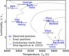 |
Fig. 1 HR diagram showing the exact and “observed” positions of the ten stellar targets. Evolutionary tracks from Silva Aguirre et al. (2015) and the Sun’s position have also been included for the sake of comparison. |
The models were calculated using the CLES stellar evolution code (Scuflaire et al. 2008). The equation of state was based on OPAL 2001 (Rogers & Nayfonov 2002) using the tabulated Γ3−1 values. OPAL opacities (Iglesias & Rogers 1996) complemented with Ferguson et al. (2005) opacities at low temperatures were used. The nuclear reaction rates came from the NACRE compilation (Angulo et al. 1999) and included the revised 14N(p, γ)15O reaction rate from Formicola et al. (2004). Convection was implemented through standard mixing-length theory using solar-calibrated values of the mixing length, αMLT (Böhm-Vitense 1958). Atomic diffusion based on the prescription given in Thoul et al. (1994) was included in specific cases. This approach includes gravitational settling, as well as the effects of temperature and composition gradients, but neglects radiative accelerations (see also Thoul & Montalbán 2007, for a review of this and other approaches). A radiative grey atmosphere using the Eddington approximation (e.g. Unno & Spiegel 1966) was included in most models and extended from the photosphere, T = Teff, to an optical depth of τ = 10-3. The fundamental properties of the targets are given in Table 3, where the models are sorted according to mass (for reasons which will become apparent later on).
In most cases, the pulsation modes were calculated with InversionKit 2.11, using 4th order calculations, various sets of equations involving either Lagrangian and Eulerian pressure perturbations, and the mechanical boundary condition δP = 0. For two of the models, the ADIPLS code (Christensen-Dalsgaard 2008a) was used instead in order to apply an isothermal boundary condition since this boundary condition is not currently implemented in InversionKit. This was used as a way to simulate surface effects, i.e. offsets between observed and modelled frequencies which occur as a result of our poor modelling of the near-surface layers of the star (e.g. Kjeldsen et al. 2008), and to attenuate the fact that the atmosphere was truncated in one of the models. The frequencies are given in Appendix A.
Fundamental properties of the stellar targets.
In order to test the effects of different physical assumptions, a number of models came in pairs and a triplet in which at least one of the properties was modified. These model groupings can easily be recognised in Table 3 since their members have the same masses. Hence, Aardvark and Elvis differ according to age and boundary condition on the pulsation modes. The main difference between Henry and Izzy is that the latter was calculated with atomic diffusion as prescribed in Thoul et al. (1994) and has a slightly different metallicity. Blofeld and Diva have different abundance mixtures, slightly different metallicities, a different treatment of the atmosphere, and different boundary conditions for the pulsation modes. Furthermore, Blofeld includes atomic diffusion whereas Diva does not. In the last group of stars, Jam is significantly younger, and George has a different overshoot parameter.
2.2. Generating “observational” data
From the above theoretical values, a set of “observational” data was produced by incorporating noise. These data included classical parameters, namely Teff, L/L⊙ and [Fe/H], and seismic constraints, which included individual frequencies as well as Δν, the average large frequency separation, and νmax, the frequency of maximum oscillation power. These “observational” data and associated error bars were then made available to the hounds through a dedicated website2 and are given in Table 1 for the global properties, and Tables A.1 to A.3 for the individual frequencies. A detailed description of how the error bars were chosen and the noise added is given in the sections that follow.
2.2.1. Global parameters
Estimates of the global or average seismic parameters νmax and Δν were provided as guideline data. We took the pristine values (νmax was obtained using Eq. (1) and Δν was calculated via a least-squares fit to the model frequencies) and added random Gaussian noise commensurate with the typical precision in those quantities expected from the analysis of a one-month dataset (i.e. 5% in νmax; 2% in Δν). We note that detailed modelling was performed by the hounds using the individual frequencies, which have a much higher information content than the above average/global seismic parameters. The pristine effective temperatures and metallicities [Fe/H] were perturbed by adding Gaussian deviates having standard deviations of 85 K and 0.09 dex (again, as per the assumed formal uncertainties). Finally, we assumed a 3% uncertainty on luminosities from Gaia parallaxes, most of which is due to uncertainty in the bolometric correction.
2.2.2. Pulsation frequencies
Each artificial star’s fundamental properties (Teff, M and R) were used as input to scaling relations from which the basic parameters of the oscillation spectrum were calculated, and from there, the expected precision in the frequencies.
The dominant frequency spacing of the oscillation spectra is the large separation Δν. In main-sequence stars, each Δν-wide segment of the spectrum will contain significant power due to the visible ℓ = 0, 1 and 2 modes, and, in the highest S/N observations, will contain small contributions from modes of ℓ = 3. The integrated power in each segment will therefore correspond to the power due to the radial mode multiplied by the sum of the visibilities (in power) over ℓ.
Let us define Amax to be the equivalent radial-mode amplitude at the centre of the p-mode envelope, i.e. at νmax, the frequency of maximum oscillation power. This frequency is calculated according to (e.g. Kjeldsen & Bedding 1995; Belkacem et al. 2011) 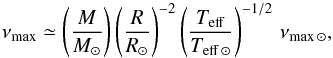 (1)with the commonly adopted solar values given in Table 4.
We also define the factor ζ to be the sum of the normalised mode visibilities (in power), i.e.,  (2)where V0 = 1 (by definition). The visibilities for the non-radial modes are largely determined by geometry. Here, we adopt values of V1 = 1.5, V2 = 0.5 and V3 = 0.03 (see Ballot et al. 2011).
Reference values.
If we re-bin the power spectrum into Δν-wide segments, the maximum power spectral density in the segment at the centre of the spectrum will be 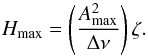 (3)We used the scaling relations in Chaplin et al. (2011) to calculate Amax and hence Hmax for each artificial star using the fundamental properties of the models as input and assuming observations were made with the Kepler instrumental response, which affects the mode amplitudes. We note that the responses of CoRoT and PLATO are similar, while that of TESS is redder, implying lower observed amplitudes.
A Gaussian in frequency provides a reasonable description of the shape of the power envelope Henv(ν) defined by the binned spectrum. We used the scaling relations in Mosser et al. (2012) to calculate the full width at half maximum (FWHM) of the Gaussian power envelope of each star, and hence the power Henv(ν) in the envelope as a function of frequency (that power being normalised at the maximum of the envelope by Hmax).
Description of hounds in group 1 (forward modelling).
Estimates of the frequency-dependent heights H(ν) shown by individual radial modes were calculated according to (e.g. Campante et al. 2014) 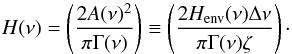 (4)Here, Γ(ν) are the fwhm linewidths of the individual oscillation peaks. Frequency dependent linewidth functions were fixed for each star using Eq. (1) in Appourchaux et al. (2014) and Eq. (2) in Appourchaux et al. (2012).
Next, the background power spectral density, B(ν), across the frequency range occupied by the modes is dominated by contributions from granulation and shot noise. We used the scaling relations in Chaplin et al. (2011) to estimate the frequency dependent background of the stars, assuming each was observed as a bright Kepler target having an apparent magnitude in the Kepler bandpass of Kp = 8. We note that PLATO 2.0 will also show similar noise levels. From there we were able to calculate a frequency dependent background-to-height (radial-mode equivalent) ratio for each star, i.e. (5)The expected frequency precision in the radial modes is then given by (Libbrecht 1992; Toutain & Appourchaux 1994; Chaplin et al. 2007)
 ![Mathematical equation: \begin{equation} \sigma(\nu) = \left(\frac{\mathcal{F}[\beta(\nu)]\Gamma(\nu)}{4\pi T}\right)^{1/2}, \label{eq:sig} \end{equation}](/articles/aa/full_html/2016/08/aa27987-15/aa27987-15-eq191.png) (6)where we assumed continuous observations spanning T = 1 yr, and the function in β(ν) is defined according to
(6)where we assumed continuous observations spanning T = 1 yr, and the function in β(ν) is defined according to ![Mathematical equation: \begin{equation} \mathcal{F}[\beta(\nu)] = \sqrt{1+\beta(\nu)} \left(\!\!\sqrt{1+\beta(\nu)}+\sqrt{\beta(\nu)}\right)^3. \label{eq:fsig} \end{equation}](/articles/aa/full_html/2016/08/aa27987-15/aa27987-15-eq194.png) (7)Estimation of the frequency precision in the non-radial modes depends not only on the non-radial mode visibility (which changes β(ν) relative to the radial-mode case), but also on the number of observed non-radial components and their observed heights (which depends on the angle of inclination of the star) and on how well resolved the individual components are (which depends on the ratio between the frequency splitting and the peak linewidth). While accounting for the change in β(ν) is trivial, correcting for the other factors is somewhat more complicated (e.g. Toutain & Appourchaux 1994; Chaplin et al. 2007). We could of course have simulated the actual observations, and applied our usual analysis techniques to extract frequencies and uncertainties to pass on for modelling. However, for this exercise we deliberately sought to avoid conflating error or bias from the frequency extraction with error or bias from the modelling. We therefore adopted an empirical correction factor eℓ for each angular degree ℓ based on results from fits to the oscillation spectra of several tens of high-quality Kepler targets. These factors can be regarded as representative; values for individual stars will vary, depending on the specific combination of individual stellar and seismic parameters and the inclination angle of the star.
(7)Estimation of the frequency precision in the non-radial modes depends not only on the non-radial mode visibility (which changes β(ν) relative to the radial-mode case), but also on the number of observed non-radial components and their observed heights (which depends on the angle of inclination of the star) and on how well resolved the individual components are (which depends on the ratio between the frequency splitting and the peak linewidth). While accounting for the change in β(ν) is trivial, correcting for the other factors is somewhat more complicated (e.g. Toutain & Appourchaux 1994; Chaplin et al. 2007). We could of course have simulated the actual observations, and applied our usual analysis techniques to extract frequencies and uncertainties to pass on for modelling. However, for this exercise we deliberately sought to avoid conflating error or bias from the frequency extraction with error or bias from the modelling. We therefore adopted an empirical correction factor eℓ for each angular degree ℓ based on results from fits to the oscillation spectra of several tens of high-quality Kepler targets. These factors can be regarded as representative; values for individual stars will vary, depending on the specific combination of individual stellar and seismic parameters and the inclination angle of the star.
The model computed eigenfrequencies of the star are νnℓ; we therefore estimated formal uncertainties on each frequency using  (8)where e0 = 1.0, e1 = 0.85, e2 = 1.60 and e3 = 6.25. This takes no account of whether a mode would in principle be detectable in the observed spectrum. Having first applied a coarse cut to the frequency list of a given star by removing frequencies having σnℓ> 5 μHz, we then ran mode detection tests (Chaplin et al. 2002, 2011) on the remaining frequencies using their predicted background-to-height ratios
  (9)and linewidths Γnℓ = Γ(νnℓ) as input, each time assuming T = 1 yr. Only those modes that passed our tests were retained (a 1% false-alarm threshold) to give a final list of frequencies νnℓ and formal uncertainties σnℓ for each star. These selected frequencies were perturbed by adding random Gaussian deviates having a standard deviation equal to σnℓ, to yield the “observational” frequencies that were passed to the modellers.
3. The hounds
The hounds were divided into two main groups. The first group applied a forward modelling approach to find optimal models, stellar properties, and associated error bars. The second group fitted the acoustic glitch signatures to characterise the base of the convection zone. One team of hounds, KV and HMA, applied both strategies and therefore appears in both groups. Finally, some other hounds applied inverse techniques as will be described below.
3.1. Group 1: forward modelling approach
The members of this group used various forward modelling strategies to find optimal models that reproduce the “observational” data, including the detailed seismic information provided. From these models, they found various properties of the star, namely mass, radius, density, log (g), and age. Some of the members of this group also provided the acoustic and physical radii and/or depths of the base of the convection zone. The main differences between the strategies applied by the different hounds concern: 1) the search algorithm (or optimisation procedure); 2) the stellar evolution codes along with the choice of physics; and 3) the exact choice of observational constraints used. This is summarised in Table 5. A slightly more detailed description is given in the following paragraphs. We also note that a number of the methods applied here have also been used in the KAGES project and are consequently described in greater detail in Silva Aguirre et al. (2015).
Several of the hounds (typically those who used frequencies as opposed to ratios) included surface corrections on the model frequencies. Typically, such corrections are negative, i.e. the model frequencies need to be decreased to match the observations. However, in a number of cases the hounds had to increase their model frequencies to match the provided frequencies. This is perhaps not entirely surprising since the “observed” frequencies come from models and not from stars with true surface effects.
GOE.
This approach involves several steps:
-
1.
Obtaining initial estimates of the model parameters anduncertainties using a pre-computed grid of models. The classicaland global seismic parameters are used when performing thisstep.
-
2.
Generating ten initial guesses that populate these parameters within their uncertainties and with mixing-lengths sampled uniformly between 1.2 and 2.4. The best-fitting parameters are also included as an eleventh guess.
-
3.
Using MESA’s built-in Nelder-Mead method (also known as a downhill simplex method or an amoeba method) to optimise the above 11 choices. All of the classical constraints, namely L, Teff, and [Fe/H], as well as individual frequencies including the one-term version of the surface corrections from Ball & Gizon (2014) were used in this process.
-
4.
Gathering the above samples into one comprehensive sample. The true global optimum is used as the best-fit, and uncertainties on the model parameters are derived from surfaces of constant χ2. To boost numbers, points beyond the
 surfaces were rescaled by the square root of their χ2 distance.
 -
5.
Finding uncertainties on derived parameters by linearising about the best-fitting model, using exp(−χ2/ 2) as weights.
The above models included overshoot based on Herwig (2000) and atomic diffusion as prescribed in Thoul et al. (1994), even for massive stars.
YMCM.
In the Yale-Monte Carlo Method (YMCM), a set of relevant models is calculated for each of the stellar targets based on a Monte Carlo analysis. Individual frequencies including a scaled solar surface correction term were fitted to observations, as were the classical constraints, including L. Frequency ratios (based on uncorrected frequencies) were subsequently used to check the results. No diffusion or overshoot was used in the models (which is expected to affect the base of the convection zone). Little evidence for a surface term was found.
ASTFIT.
In the ASTEC Fitting method (ASTFIT), grids of evolutionary tracks are used to interpret the data. None of the models takes atomic diffusion into account, and convective-core overshoot is not included. A fixed enrichment law with ΔY/ ΔZ = 1.4 was used when constructing the grids. Best-fitting models along the relevant tracks were found using homologous transformations, and were obtained by interpolation. These models were selected according to individual frequencies, which were corrected for surface effects using a scaled version of the solar surface term (Christensen-Dalsgaard 2012; we note that the implementation of this term is slightly different to what is applied in the YMCM pipeline). The luminosity was not used when finding optimal models. Average results were obtained from individual results weighted according to exp(−χ2/ 2), where  , the quantity
  being a reduced χ2 based on the frequencies, and
  a χ2 value on the classic observables (excluding the luminosity).
YL.
A Levenberg-Marquardt approach was used to fit the seismic and classic constraints, namely individual frequencies with surface corrections based on Kjeldsen et al. (2008), and L, Teff, and [Fe/H]. Stellar models were calculated on the fly and included atomic diffusion as prescribed in Michaud & Proffitt (1993). The effects of overshoot were tested in some of the more problematic stars, but the final list of results is based on models without overshoot. This approach provides both the best-fitting properties relevant to the grid (namely mass, age, metallicity Z/X, helium abundance Y, and mixing length) and the uncertainties on the properties. Other properties, such as R,  , log (g), rBCZ/R, are derived from the best-fitting models and consequently do not have error bars.
AMP.
The Asteroseismic Modeling Portal (AMP) searches the stellar parameter space using a parallel genetic algorithm. Stellar models and associated frequencies are calculated on the fly in this approach. These models include the effects of helium diffusion (Michaud & Proffitt 1993), but not overshoot. The same AMP configuration used in Metcalfe et al. (2014) was also applied here; the updated physics and fitting methods described in Metcalfe et al. (2015) were not employed. In particular, individual frequencies (including surface corrections based on Kjeldsen et al. 2008) and frequency ratios were simultaneously used when searching for best-fitting models. Likelihood-weighted mean values and associated standard deviations were then obtained from the calculated models. These properties are consistent with the properties of individual models identified by the genetic algorithm. We note that Felix and Diva were the least well fitted.
BASTA.
The BAyesian STellar Algorithm (BASTA) consists in mapping out the posterior probability distribution function by scanning a pre-computed grid of stellar models. It uses Teff, and [Fe/H] as constraints, but not luminosity. Given that the method relies on frequency ratios, frequency corrections for surface effects were not used. Some of the grids included atomic diffusion as based on Thoul et al. (1994), and some of them took overshooting into account using an exponential decay on the convective velocities in the overshooting region (cf. Weiss & Schlattl 2008; Silva Aguirre et al. 2011). A fixed enrichment law with ΔY/ ΔZ = 1.4 was used in the grids. A number of properties and associated, non-symmetric error bars are provided, but the acoustic radii of the base of the convection zones had to be extracted from best-fitting models.
MESAastero.
The MESAastero procedure is a two-step process: the first step involves generating grids of models in the vicinity of the different stellar targets. This provides good starting points for the second step, which is an automated search based on the MESA built-in Nelder-Mead method, where models are calculated on the fly. The uncertainties were calculated as the average distance of the set of points with  , where
  is the χ2 value of the best-fitting model. If the resulting χ2 landscape from the first simplex run did not look reasonably well sampled (e.g. it was single sided with respect to the minimum), additional simplex runs were carried out using different starting values. This ensured that a global minimum was found and robust uncertainties could be derived. The observational constraints used to find best-fitting models were Teff, [Fe/H], and individual frequencies. The surface correction recipe from Kjeldsen et al. (2008) was included for Aardvark, Elvis, Henry, and Izzy. The models were constructed using [Fe/H], M, and αMLT as free parameters, and used a fixed enrichment law with ΔY/ ΔZ = 1.4. They included an exponential prescription for overshoot based on Herwig (2000), but not diffusion.
V&A, grid.
In the approach used here, 1000 evolutionary tracks with randomly selected model properties in appropriate ranges were computed for each stellar target. One best model for each evolutionary track was obtained by fitting the uncorrected model frequencies to the given frequencies. In this way, we obtained an ensemble of models with different masses, initial compositions, mixing-lengths and ages. From this ensemble of models, a χ2 map was calculated, thereby yielding best-fitting properties and associated error bars. The χ2 values were based on L, Teff, surface metallicity, and the average large and small frequency separations (as opposed to individual frequencies). The models included diffusion of He and heavy elements (Thoul et al. 1994), except for higher mass targets (namely Diva, Felix, George, and Jam). However, they did not include overshoot.
3.2. Group 2: glitch fitting analysis
The second group of hounds fitted the acoustic glitch signatures in order to obtain the acoustic depths of the base of the convection zone and that of the He II ionisation zone or the nearby Γ1 peak. This type of method relies on the fact that sharp features in the acoustic structure of the star, such as the transition from a radiative to a convective zone or the presence of an ionisation zone, lead to an oscillatory pattern in the frequency spectrum. The period of this pattern gives the acoustic depth of the feature, whereas the amplitude and rate of decrease with frequency is related to the amplitude of the feature and to its “sharpness”, i.e. whether the feature corresponds to a discontinuity on the first, second, or a higher derivative of the acoustic profile (e.g. Monteiro et al. 1994).
Fitting acoustic glitch signatures differs from the forward modelling approach in that it focuses on very specific information contained within the pulsation spectrum rather than trying to fit the spectrum as a whole. Furthermore, it does so directly without making comparisons with theoretical predictions from models (except for interpreting the amplitude of the feature in terms of He abundance; see e.g. Verma et al. 2014b), thereby making the results model-independent. In contrast, the forward modelling approach is indirect and model-dependent since it ends up implicitly comparing glitch signatures present in the observations to those obtained in theoretical models. Furthermore, these features may be drowned out by other features present in the pulsation spectra.
The acoustic depths obtained by these hounds were subsequently converted to acoustic radii using the total acoustic radii. The associated error bars were calculated as the sum of the error bars on the acoustic depths and those coming from the total acoustic radii. In keeping with the approach taken in the glitch fitting analysis, the total acoustic radii were deduced from the large frequency separations. However, rather than using the coarse values provided, the frequency separations were recalculated via a least-squares fit to all of the “observed” frequencies using the provided uncertainties to find appropriate weights. These values, Δνrecalc., along with the uncertainties deduced from the least-squares fit (which only keeps track of how the uncertainties on the frequencies propagate to the final result, but does not take into account how well the frequencies fit a linear trend), and the resultant acoustic radii are listed in Table 6. A comparison between Tables 1 and 6 confirms the improved accuracy of Δνrecalc..
Comparison between different evaluations of the acoustic radius.
Description of hounds in group 2 (glitch fitting analysis).
It is important to bear in mind that significant discrepancies can appear when calculating the acoustic radii of stars. This is illustrated by the differences between the third and fourth columns in Table 6, which contain two different calculations of the acoustic radius. These differences likely stem from the fact that τTot. represents an asymptotic value whereas 1/2Δν is based on modes of finite radial order. Another source of error includes differences in the exact definition of the radius used as an upper integration bound in the definition of τTot. (e.g. Hekker et al. 2013). Such differences will also affect the values given for the acoustic depth of the base of the convection zone. In order to derive the acoustic radius in a physically sound way, one would need to linearly extrapolate the squared sound speed c2 from the outer regions of the adiabatically stratified portion of the convection zone to the place where c2 would vanish, and integrate dr/c to this point (Houdek & Gough 2007). In what follows, we take a more pragmatic approach that consists in comparing the acoustic radii rather than the depths of the base of the convection zone. Indeed, as pointed out in Ballot et al. (2004), this approach mostly cancels out any differences in the precise definition of the stellar radius used in calculating the acoustic depth.
Table 7 lists the specific frequency combinations that were used to find glitch signatures. Relevant references are also provided. The following paragraphs then give a few more details on the methodologies of the various hounds from this group.
V&A, glitch.
The approach taken here is method C of Verma et al. (2014b). In this method, both the smooth and oscillatory glitch-related components are simultaneously fitted directly to the frequencies. A Monte Carlo approach was used to obtain the uncertainties on the glitch parameters. This involved constructing histograms of the parameters deduced from multiple realisations of the data.
HRC.
Applied an MCMC approach to fitting the second frequency differences, thereby obtaining the posterior probability distribution function of the glitch parameters. This allowed him to obtain optimal values along with their associated error bars.
GH.
Fitted glitch signatures to second frequency differences. Specifically, this analysis includes both ionisation stages of helium (unlike the methods from the other glitch-fitting hounds, which only include a single signature for both ionisation stages) and adopts Airy functions and a polytropic representation of the acoustic potential in the stellar surface layers to account more realistically for the contribution from the He I glitch, which for stars with surface temperatures similar to the Sun lies partially in the evanescent region of acoustic modes. This leads to deeper (greater) acoustic depths, since these are measured relative to the acoustic radius determined from linearly extrapolating c2 to the place where it vanishes (as describe above) as opposed to the location indicated by 1/2Δν. Accordingly, the acoustic radii reported throughout the article for this method will be underestimated owing to the use of 1/2Δν in the conversion from acoustic depths to acoustic radii. For the parameters, which relate the fitting coefficients of the He I glitch to those of the He II glitch, the constant solar values of Houdek & Gough (2007) were adopted for all model fits. Finally, the error bars were deduced from a Monte Carlo analysis, much like what was done by V&A, glitch.
AM
3. Also fitted the second frequency differences. Once more, the error bars were deduced from a Monte Carlo analysis.
3.3. Others: inversion techniques
In addition to these two main groups of hounds, GB and DRR applied the mean density inversions described in Reese et al. (2012), but had different strategies for selecting the reference models. For each target, GB selected a reference model via the Levenberg-Marquardt algorithm, using the average large and small frequency separations, r01 frequency ratios, and Teff as constraints (e.g. Buldgen et al. 2015). Accordingly, the reported uncertainties only take into account how the observational uncertainties on the frequencies propagated through the inversion process onto the mean densities. DRR used an inversion pipeline to select reference models from a grid using log (L), Teff, νmax, Δν as constraints. For the last parameter, the coarse values provided with the data were used, and Δν was not recalculated. The constraint on [Fe/H] was discarded as it could lead to some of the targets having no reference models. Inversion results from each reference model were combined after being weighted by the χ2 value associated with the constraints used to select the reference models. Accordingly, the error bars take into account the observational error propagated through the inversion procedures and the scatter between the results from the different models.
4. Results
In this section, we compare the results obtained by the various hounds with the actual properties of the artificial stars. We start by introducing various average error and bias measurements, which helps assess the quality of the results and reported uncertainties. This is followed by a comparison of the results obtained for global properties before focusing on the properties related to the base of the convection zone and the He II ionisation zone.
4.1. Average errors and biases
In order to summarise the quality of the results it is helpful to introduce the following average error measurements, 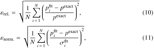 where p is a given property, the superscripts “exact” and “fit” refer to the exact and fitted values, σ the estimated error bar (or the average if the error bar is not symmetric), N the number of relevant cases, and i each particular case. In what follows, these errors will be averaged over
-
particular stars;
-
particular hounds;
-
over all the stars and hounds.
The error from Eq. (10), which we will call the average relative error, gives a measure of the relative accuracy with which a particular parameter is determined, whereas the error from Eq. (11), the average normalised error, is used to see how realistic the reported error bars are. High values indicate that the error bars are underestimated, low values mean the error bars are overestimated, and values close to unity correspond to well-estimated error bars. In cases, where a particular value is not provided, it is excluded from the average relative error. If an error bar is not provided, the associated value is excluded from the average normalised error.
In addition, we also define biases, which come in the same two flavours as above:  These are useful for detecting a systematic offset between fitted results and the true values. We note in passing that the scatter, σ, of the results around the bias is given by the formula
  (14)where j could stand for “rel.” or “norm.”.
4.2. Global properties
The most important global properties are radius R, mass M, and age t. They are key properties in stellar evolution and have a direct impact on the study of exoplanetary systems and on the study of galactic stellar populations. We also decided to include two other properties, namely the mean density and log (g), g being the surface gravity. Although it is straightforward to derive these properties from M and R, their error bars cannot be deduced directly from the error bars on M and R alone given the correlations between these two quantities.
Tables 8 to 12 list the results from the various hounds and the associated average errors and biases. Figures 2 to 6 illustrate these results.
Fitted values for the radius in solar units, R, and associated average errors and biases.
Fitted values for the mass in solar units, M, and associated average errors and biases.
Fitted values for the age in Gyr, t, and associated average errors and biases.
Fitted values for log (g) in dex and average errors and biases for g (in cm s-2).
Fitted values for in g cm-3, and associated average errors and biases.
The relative error bars on the radius, mass, and age, averaged over all of the stars and relevant hounds, are 1.5%, 3.9%, and 23%, respectively. The first two are well within the requirements for PLATO 2.0 and are comparable to the results recently obtained in the KAGES project (Silva Aguirre et al. 2015). The age, on the other hand, is determined with a higher uncertainty than was achieved in Silva Aguirre et al. (2015). However, we note that in the present work, the uncertainties are calculated with respect to the exact solutions rather than as a dispersion between different results. If, however, the exact solutions are replaced by the average of the results obtained by the hounds, then the overall relative error bar (averaged over all of the stars and hounds) becomes 20%, which is closer to the result obtained by Silva Aguirre et al. (2015) who found 14%. Also, the proportion of massive (and problematic) stars seems to be slightly higher in the present sample. Nonetheless, it is important to note that the age estimates for Aardvark and Elvis, the two stars that match the PLATO 2.0 reference case quite well, are on average accurate to within 10%, thereby satisfying the requirements for PLATO 2.0.
It is also interesting to look at how well the error bars were estimated. On the whole, the error estimates are quite reasonable; there are only a few outlying cases. In some cases, the error bars were underestimated, for instance on the age by YL and on the mean density by GB. In YL’s case, the difference may be related to the fact that she is using a Levenberg-Marquardt approach, which is more prone to getting stuck in local minima. In GB’s case, inversions are applied to a single reference model. Hence, his error bars only take into account the errors on the frequencies as they propagate through the inversion. However, such errors do not take into consideration that the reference model may be sub-optimal (thus requiring non-linear corrections). DRR also applied inversions, but to a set of reference models selected according to classical constraints. Hence, his error bars include the scatter between the results from the different reference models and are thus more realistic. Nonetheless, in both cases, the error bars do not account for mismatches between averaging kernels and relevant target functions. We also note that GB included a surface correction term in his inversions, whereas DRR did not. This, in fact, leads to worse results for all of the stars except Aardvark, owing to the reduced quality of the averaging kernels, as indicated by further tests by GB. Inversions naturally mitigate surface effects, so including a surface correction term yields little improvement while degrading the quality of the averaging kernel.
4.2.1. Comparisons between similar stars
Aardvark and Elvis.
Aardvark and Elvis differ in age (Aardvark is approximately half the age of Elvis) and in the use of an isothermal boundary condition on the pulsations (this condition was applied in Elvis but not in Aardvark). Both stars were well characterised by the hounds with slightly better results for Aardvark. Interestingly, the average relative error on the age was slightly smaller on Aardvark, even though the star is younger, thereby also implying an absolute error on the age more than twice as small. This is somewhat surprising because the central hydrogen abundance decreases roughly linearly in time over the main sequence, thereby leading to the expectation that the absolute age error should be similar at all ages on the main sequence. Hence, one would expect the relative error to be larger for younger stars. As mentioned above, these stars are the closest to PLATO’s reference case, and the results for these stars satisfy all of the requirements for PLATO 2.0.
Felix, George, and Jam.
It is also interesting to see which stars were the most problematic. In this particular case, the star Felix proved to be challenging for a number of hounds and was even excluded by one of them. We note that George and Jam also yielded poor results and not all of the hounds proposed results for these stars. Their average relative errors show substantial scatter between the different hounds, and the average relative biases were also significant. In the case of the age, the error bars were often highly underestimated.
The common factor between these stars is their high mass, 1.33 M⊙. High mass leads to various phenomena, which make these stars more difficult to model and their pulsations more difficult to interpret. For instance, these stars are hotter and lead to shorter mode lifetimes and, thus, larger error bars on the frequencies. Furthermore, these stars contain convective cores, which may result in sharp density gradients. Different stellar evolution codes use different criteria for defining the boundary of the convective core (e.g. Gabriel et al. 2014), different core overshoot prescriptions, and different numerical approaches, all of which affect the size of the convective core and its transition to the radiative region above. Accordingly, there can be large discrepancies in the sizes of convective cores in models from different evolution codes.
It is interesting to compare these stars. The main difference between Felix and George is the higher overshoot parameter in the latter. Although the two have the same mass, it is interesting that, on the whole, the mass of Felix was underestimated whereas the mass of George tended to be overestimated. Even more dramatic are the age differences between the two obtained by the various hounds. Hence, on average, Felix was found to be 0.79 Gyr older and 0.082 M⊙ lighter than George (if we limit ourselves to hounds who gave results for both stars), even though both have the same mass and nearly the same age. Of course, it is normal that the mass and age are anti-correlated, because lighter stars evolve more slowly and will therefore be older for a given evolutionary stage. Jam had a similar overshoot parameter to Felix but was substantially younger. On the whole, Jam seemed to yield better results (with substantially less scatter on the mass), but obtaining accurate ages for this star still proved to be difficult.
Blofeld and Diva.
The stars Blofeld and Diva also proved to be problematic. Although these stars share the same mass (1.22 M⊙), they are different in a number of ways. Indeed, the distinguishing features of Blofeld include a different heavy abundance mixture (AGS05), diffusion, a truncated atmosphere, and the use of an isothermal boundary condition on the pulsations to reduce the effects of the truncated atmosphere. In contrast, Diva, is much more like the other stellar targets.
It is interesting to look at each of the distinguishing features of Blofeld and discuss how likely they are to affect the results from the hounds. The truncated atmosphere can lead to important surface effects. However, as pointed out above, the isothermal boundary condition reduces these effects; accordingly, some of the hounds reported rather small surface effects on the frequencies. We note in passing that Elvis did not seem to be much affected by the isothermal boundary condition (but unlike Blofeld, its atmosphere was not truncated). The composition can also be a source of error. SB reran the YMCM pipeline on Blofeld using the correct mixture (AGS05 as opposed to Grevesse & Sauval 1998 as used in the previous run). The results are shown in Table 13. Apart from the age (which is likely to be affected by a fortuitous agreement with the original result judging from its extreme accuracy), all of the stellar properties are determined with increased accuracy, thereby highlighting the importance of using the correct composition.
Finally, atomic diffusion, in which radiative accelerations are neglected, is expected to be problematic given the relatively high mass of this star. Indeed, this tends to over-deplete surface heavy abundances compared to observations in higher mass stars. Radiative accelerations counteract this effect by levitating heavy elements to specific regions of the star, which in turn affects local opacities and may lead to supplementary convection zones (e.g. Richard et al. 2001). In addition, element accumulation can lead to double-diffusive convection, another means by which elements can be redistributed within stars (e.g. Deal et al. 2016). Given that radiative accelerations were not taken into account by the various diffusion prescriptions used in the present exercise, several of the hounds (VSA and V&A) only included atomic diffusion up to a certain mass threshold which is close to Blofeld’s mass, thereby potentially leading to greater discrepancies in the results.
Original versus new YMCM results (with the correct mixture, i.e. AGS05) for Blofeld.
A comparison of the results for both stars showed that Blofeld had better age and surface gravity estimates, whereas Diva had better mass and mean density estimates. The radius estimates for the two stars were very similar in quality. Interpreting these differences is not straightforward. Surface effects are expected to affect “structural” properties (namely, M, R, , log (g)), but the results are not clear cut. However, as argued above, surface effects may not be the dominant factor in Blofeld. Diffusion is also expected to make it more difficult to estimate the age of Blofeld, but the opposite is true in the present case. It is not clear why this is so, although we do note that the older star has a greater relative error as was the case for Aardvark and Elvis.
Henry and Izzy.
The main difference between Henry and Izzy is the fact that the former includes diffusion. However, in terms of results, both were fairly similar, with results for Henry being slightly better on structural properties (for the most part) and results for Izzy being better on the age. Hence, diffusion seems to have a small impact on the results, as is expected for stars of this mass.
4.3. Properties related to the base of the convection zone
We now turn our attention to properties related to the base of the convection zone. As stated earlier, the hounds were asked to provide the fractional radius of the base of the convection zone (for those carrying out grid modelling) as well as the acoustic radius or depth of the base of the convection zone along with the acoustic radius of the star.
 |
Fig. 2 Fitted results for the radius. Each panel corresponds to a stellar target, the columns in each plot to particular hounds, and the horizontal dotted line to the true value. |
 |
Fig. 3 Fitted results for the mass. |
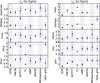 |
Fig. 4 Fitted results for the age. |
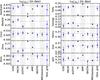 |
Fig. 5 Fitted results for log (g). Different symbols and colours represent different techniques for obtaining the result. |
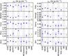 |
Fig. 6 Fitted results for |
Tables 14 and 15 list the results obtained for the fractional radius of the base of the convection zone, rBCZ/R, and the acoustic radius of the base of the convection zone, τBCZ. The fractional radius can only be obtained from a forward modelling approach since it is not an acoustic variable. In contrast, the acoustic radius can be found through both forward modelling and glitch fitting. It is also interesting to note that one of the hounds applied both approaches. These results have been kept as separate entries in Table 15 and are shown separately in Fig. 8 under the headers “V&A, grid” for the grid modelling and “V&A, glitch” for the glitch fitting.
Fitted values for rBCZ/R and associated average errors and biases.
Fitted values for τBCZ (in s) and associated average errors and biases.
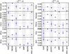 |
Fig. 7 Fitted results for rBCZ/R. |
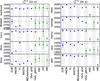 |
Fig. 8 Fitted results for τBCZ (in s). |
Overall, the fractional radius at the base of the convection zone is fairly well fitted, with a global relative average error at 3.2%. This is, however, approximately twice as large as the errors on the stellar radius. It is tempting to think that this larger error on rBCZ/R is an accumulation of both the errors on the radius and those on the internal structure. However, this simple reasoning does not account for the fact that for some stars, the error on R is larger than on rBCZ/R. What really emerges from a detailed comparison is that the radius is more consistently determined, whereas rBCZ/R seems to be less consistent: some results were very accurate and others very inaccurate.
It is then interesting to have a detailed look at the results for τBCZ. Here, the errors are much larger with a very clear dichotomy between the two approaches. Apart from some outliers, forward modelling produces consistent and reliable results. In contrast, glitch fitting seems to be more prone to finding spurious solutions (see e.g. Diva and Izzy). Nonetheless, one should not forget that in the present case, forward modelling benefits from the fact that it relies on models with similar physical ingredients to those used by the hares when constructing the target stars. If real stars were used, the errors in the forward modelling would likely increase owing to supplementary physical phenomena that are not currently included in stellar evolution codes. In contrast, the glitch-fitting approach is model-independent and would not be affected in the same way. We also note that the stars that were problematic for one method were not always problematic for the other. Blofeld turned out to be one of the most well-fitted stars by glitch analysis, in spite of diffusion and the different mixture that seemed to affect forward modelling. In contrast, Coco proved to be difficult to model for some of the glitch-fitting hounds, even though it was very straightforward to model using forward modelling. It is also interesting to point out that in some cases, namely for Coco and Henry, “V&A, glitch” did not make the same mistakes as the other hounds who applied glitch fitting. This can be explained by the fact that there are multiple solutions to the glitch fitting problem and that “V&A, glitch” was helped by “V&A, grid” when selecting the correct solution. Nonetheless, for Diva and Izzy, “V&A, glitch” and “V&A, grid” found different solutions. We also note that GH managed to find the correct solution for Coco, and gave much larger and, hence, more realistic error bars for George as a result of finding a bi-modal solution (although the second mode seems to go the wrong way, judging from the error bars). It is not entirely clear why GH obtained better results than HRC and AM for Coco given that all three used second frequency differences.
In order to understand these spurious solutions found by the glitch fitting approach, we looked at the sound-speed profile as a function of acoustic radius to see if there are other features in the model that could produce a glitch signature. A first analysis showed that none of the spurious solutions corresponded to a sharp acoustic feature located elsewhere in the star. However, a number of spurious solutions appeared to be complements (i.e. acoustic depths rather than radii) of either the actual solution or of approximately the He II ionisation zone, thereby implying an aliasing problem. For instance, for Diva, Felix, George, and Izzy, the complement to the solution was found by some of the hounds. Some of the solutions for Coco and Felix were complements to the He II ionisation zone. Both of these situations are illustrated in Fig. 9 where the dc/ dτ profile and its complements are plotted for Felix. Strictly speaking, aliasing such as that illustrated in Fig. 6 of Mazumdar & Antia (2001) is only applicable for an analysis based on a single ℓ value, but in practice – unless the errors on the frequencies are very small – it will manifest itself even when multiple ℓ values are used. In some cases, even with the knowledge of the “correct” value, it may not be possible to find a corresponding peak in the distribution of glitch values. It was also noted in Verma et al. (2014a) that fits to acoustic glitches tend to deteriorate as the mode frequencies approach the Brunt-Väisälä frequency, a typical situation in the more massive stars due to sharp gradient that forms above their convective core. A possible explanation for this is the fact that the asymptotic relation used to describe the frequencies is no longer valid, thereby leading to deviations from the form of the fitting function used in the glitch analysis.
Finally, no feature was found to explain the spurious solutions in Henry and Jam (although we do note that the solutions found for Jam may marginally correspond to the complement of the He II ionisation zone). Figure 10 compares the solutions for Henry to the dc/ dτ profile and its complements. A possible explanation for Henry is that the signal-to-noise ratio (S/N) for the glitch signature is too low to allow us to obtain anything meaningful. Nonetheless, it is surprising that nearly the same erroneous solution is found by more than one hound.
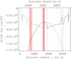 |
Fig. 9 Comparison between glitch-based solutions for the acoustic radius of the base of the convection zone in Felix (solid vertical red lines and shaded pink area for the error bars), and the dc/ dτ profile (solid black curve). The true solution, the He II ionisation zone, and the peak in the Γ1 profile, located between the He I and He II ionisation zones, are indicated by the vertical dashed blue lines at 3830 s, 5816 s, and 6041 s, respectively. The dotted and the dot-dashed green curves show dc/ dτ as a function of acoustic depth. Given the uncertainties on the determination of the total acoustic radius, the dotted curve uses τTot. whereas the dot-dashed curve uses 1/2Δν (see Table 6). The upper x-axis also uses 1/2Δν as the total acoustic radius. |
In this context, it is important to mention the role of atomic diffusion. As has been shown in previous studies (e.g. Théado et al. 2005; Castro & Vauclair 2006), atomic diffusion reduces the helium content in the convective envelope thereby leading to a helium gradient near its base and slightly modifying its location. This will then alter the amplitude of the corresponding glitch signature and may facilitate its detection in some cases (for instance in more massive stars). This will remain true even when radiative accelerations are included, as the radiative flux is unable to support this amount of helium (e.g. Vauclair et al. 1974). The fact that some of the hounds included atomic diffusion (without radiative accelerations) while others did not leads to inconsistencies. The resultant increased dispersion in the results can, however, be used to give us a first qualitative idea of the effects of neglecting physical phenomena which occur in observed stars.
4.4. He II ionisation zone and Γ1 peak
The He II ionisation zone generally leads to a stronger glitch signature than the base of the convection zone. Accordingly, all of the hounds who applied a glitch analysis returned estimates of the acoustic depth of this zone, which was subsequently converted to acoustic radii using the 1/2Δν values provided in Table 6. However, it is important to bear in mind that the glitch signature corresponds to a region that tends to be near the peak in the Γ1 profile between the He I and II ionisation zones, rather than the minimum in the Γ1 curve resulting from the He II ionisation zone, as was recently pointed out by Broomhall et al. (2014) and Verma et al. (2014a). Accordingly, in what follows we compare the results from V&A, glitch, HRC, and AM with the acoustic radius of this peak, which we denote τpeak. The analysis by GH is somewhat different because he fits both the He I and He II ionisation zones. Accordingly, his results will be compared with τHe II.
In addition to the results from the glitch analysis, V&A also sent in both τHe II and τpeak from their best-fitting models. The same values were also extracted from the actual solutions, and from the best-fitting models produced by YMCM and BASTA. All of these results are displayed in Fig. 11. Tables 16 and 17 list the results and solutions. Except for the results from GH, all of the results from the glitch analysis are in Table 17, which contains the results for τpeak.
Fitted values for τHe II (in s) and associated average errors and biases.
Fitted values for τpeak (in s) and associated average errors and biases.
Overall, the results for τHe II and τpeak are much more accurate than the results for τBCZ. This is expected given the stronger glitch signature from these features. Also, the results based on best-fitting models are more accurate than those from the glitch analysis, as was the case for τBCZ. A more detailed look shows that, except for Aardvark and Izzy, GH found lower results than all of the other hounds who applied glitch analysis. This is expected since he is fitting the He I and He II ionisation zones separately. In two cases, his results are too low. Diva can be explained by the fact that the GH analysis measures acoustic depths relative to the point where the linearly extrapolated c2 profile vanishes, as pointed out in Sect. 3.2, rather than the point corresponding to 1/2Δν, which lies below. For George, there seem to be multiple local minima, one of which corresponds to the result given here and another consistent with the results provided by the other hounds. This shows once more the limitations of local optimisation methods. Moreover, it is questionable whether the adopted solar-based parameters for relating the He I to He II glitch are still appropriate at such a high luminosity.
Once more, atomic diffusion can affect the detection of the helium ionisation zones. The helium abundance in the convective envelope is reduced by diffusion, even if radiative accelerations are present, thereby modifying the amplitude of the corresponding glitch signature (e.g. Théado et al. 2005; Castro & Vauclair 2006). Accordingly, glitch analysis will only yield the helium abundance in the convective envelope, which will differ from the helium abundance below as a result of atomic diffusion.
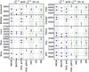 |
Fig. 11 Fitted results for τHe II and τpeak (in s). The two horizontal dotted lines correspond to the solutions (τHe II is always smaller than τpeak), and the various symbols correspond to the results from the different hounds. The type of symbol corresponds to the type of method (forward modelling or glitch analysis). |
4.5. Structural profiles
Finally, in this section we compare some of the structural profiles from the solutions and from the best-fitting models from YMCM and BASTA. A systematic investigation of all of the targets showed a mixture of results. For some of the targets, the results found by the hounds were very similar to the correct solution, whereas non-negligible differences showed up for other targets. Sharp density gradients near the core tended to be problematic and could lead to incorrect profiles in the entire core, especially for YMCM, as illustrated in Fig. 12 (upper panel). However, it is not too surprising that these features are difficult to reproduce since they only take up a small portion of the star in terms of acoustic radius and only lead to small differences in the sound-speed profile, as shown in Fig. 12 (middle panel). Also, the extent of the stellar atmospheres in the models used by BASTA were more limited than those of the stellar targets, which in turn were more limited than those of the YMCM models. This led to differences in the total acoustic radii of the various models and stellar targets (when integrating dr/c to the last mesh point) and meant that the hounds were unable to fit both the acoustic radius and the acoustic depth of features such as the He II ionisation zones or the base of the convection zone. A systematic look at the results revealed that BASTA did a better job at reproducing acoustic depths of the He II ionisation zones to the detriment of their acoustic radii, as illustrated in Fig. 12 (lower panel), whereas YMCM reproduced acoustic radii more accurately. The reason for this difference in behaviour between the two methods is not entirely clear, but it does highlight the impact of the extent of the atmosphere. Sometimes, the He II ionisation zone was not well reproduced, in terms of both physical location and depth in the Γ1 profile, as illustrated in Fig. 13. Nonetheless, in spite of these differences, the sound-speed profile remained similar between the targets and the best-fitting models in all of the cases. This is probably because of the high sensitivity of acoustic modes to the sound speed.
5. Conclusion
This article describes the results of a hare-and-hounds exercise conducted within the context of the SpaceInn network. In this exercise, simulated observational data, including detailed frequency spectra and classic observables (Teff, [Fe/H], L), for a set of ten artificial stars were provided by a group of hares. Other participants, the hounds, applied various methodologies in order to deduce the properties of these stars as well as realistic error bars. The hounds were subdivided into two main groups: the first applied forward modelling and the second relied on acoustic glitch signatures. In addition to these groups, two other hounds used inverse techniques.
The overall accuracies on radius, mass, age, surface gravity, and mean density when using forward modelling were 1.5%, 3.9%, 23%, 1.5%, and 1.8%, respectively. Furthermore, these accuracies become 1.2%, 3.2%, and 8.2% on radius, mass, and age, respectively, for the two 1M⊙ stars, thereby easily satisfying the requirements for the PLATO 2.0 mission. The stars that proved to be the most challenging were Felix, George, and Jam, owing to their high mass, and Blofeld, probably because of diffusion at a relatively high mass and/or the different abundance mixture. High-mass stars are hotter, thereby leading to shorter mode lifetimes and larger error bars on their frequencies, and contain convective cores, the sizes of which strongly depend on the various prescriptions used in stellar evolution codes. Atomic diffusion, in which radiative accelerations are neglected as is the case here, leads to depletion of heavy elements at the surface of higher mass stars (in contradiction with current observations) and is therefore usually only included in lower mass models.
Taking into account results from both forward modelling and glitch analysis, the average errors on the acoustic radii τBCZ, τHe II, and τpeak were 17%, 2.4%, and 1.9%, respectively. Furthermore, forward modelling results tended to be more accurate than those from glitch analysis, which seemed to be affected by aliasing problems in a number of cases. One possible explanation is that glitch analysis finds multiple local minima and needs prior information before the correct minimum can be selected.
 |
Fig. 12 Various structural profiles for Felix (solid blue lines) and for the relevant best-fitting models from YMCM (dotted green lines) and BASTA (dashed red lines). |
 |
Fig. 13 Γ1 profile for Elvis (solid blue lines) and for the relevant best-fitting models from YMCM (dotted green lines) and BASTA (dashed red lines). |
Overall, forward modelling seems to be the most promising way of carrying out detailed asteroseismology in solar-type stars. Nonetheless, it is – by construction – very model-dependent and will benefit greatly from the results of methods that are less model-dependent like seismic inversions, or model-independent like glitch analysis. Indeed, the present exercise only tests the ability of various asteroseismic methods to reproduce the properties of artificial stars. As such, it is unable to test the effects of hitherto unknown or poorly modelled physical phenomena present in real stars. More realistic models should include the effects of radiative accelerations, a more realistic description of convection (for instance based on 3D simulations, see e.g. Trampedach et al. 2014; Magic et al. 2015), rotation and the mixing it induces (e.g. Eggenberger et al. 2010), magnetic activity cycles, a more realistic atmosphere etc. In addition to being less model-dependent, glitch analysis is not always prone to the same difficulties as the forward modelling approach, thereby making the two methods complementary. Finally, results from one of the hounds suggest that global optimisation algorithms should be used instead of local ones in order to obtain robust error bars, given that the latter are more prone to being trapped in local minima.
This code is currently available at: http://bison.ph.bham.ac.uk/~dreese/InversionKit/
This stands for A. Mazumdar and not A. Miglio.
Acknowledgments
We thank the referee, S. Vauclair, for clarifications concerning the role of atomic diffusion, and for other comments and suggestions. DRR was funded by the European Community’s Seventh Framework Programme (FP7/2007-2013) under grant agreement No. 312844 (SPACEINN), which is gratefully acknowledged. This article made use of InversionKit and InversionPipeline, inversion software developed in the context of the HELAS and SPACEINN networks, funded by the European Commission’s Sixth and Seventh Framework Programmes. W.H.B. acknowledges research funding by Deutsche Forschungsgemeinschaft (DFG) under grant SFB 963/1 “Astrophysical flow instabilities and turbulence”, Project A18. S.B. acknowledges NASA grant NNX13AE70G and NSF grant AST-1514676. G.B. is supported by the FNRS (“Fonds National de la Recherche Scientifique”) through a FRIA (“Fonds pour la Formation à la Recherche dans l’Industrie et l’Agriculture”) doctoral fellowship. Funding for the Stellar Astrophysics Centre is provided by The Danish National Research Foundation (Grant DNRF106). The research is supported by the ASTERISK project (ASTERoseismic Investigations with SONG and Kepler) funded by the European Research Council (Grant agreement No.: 267864). The research leading to the presented results has received funding from the European Research Council under the European Community’s Seventh Framework Programme (FP7/2007-2013)/ERC grant agreement no 338251 (StellarAges). A.M. was supported by the NIUS programme of HBCSE (TIFR). VSA acknowledges support from VILLUM FONDEN (research grant 10118).
References
- Aerts, C., Christensen-Dalsgaard, J., & Kurtz, D. W. 2010, Asteroseismology, Astron. Astrophys. Library (Springer Science) [Google Scholar]
- Allen, C. W. 1973, Astrophysical quantities (Athlone Press) [Google Scholar]
- Angulo, C., Arnould, M., Rayet, M., et al. 1999, Nucl. Phys. A, 656, 3 [NASA ADS] [CrossRef] [Google Scholar]
- Appourchaux, T., Benomar, O., Gruberbauer, M., et al. 2012, A&A, 537, A134 [NASA ADS] [CrossRef] [EDP Sciences] [Google Scholar]
- Appourchaux, T., Antia, H. M., Benomar, O., et al. 2014, A&A, 566, A20 [NASA ADS] [CrossRef] [EDP Sciences] [Google Scholar]
- Appourchaux, T., Antia, H. M., Ball, W., et al. 2015, A&A, 582, A25 [NASA ADS] [CrossRef] [EDP Sciences] [Google Scholar]
- Asplund, M., Grevesse, N., & Sauval, A. J. 2005, in Cosmic Abundances as Records of Stellar Evolution and Nucleosynthesis, eds. T. G. Barnes, III, & F. N. Bash, ASP Conf. Ser., 336, 25 [Google Scholar]
- Baglin, A., Auvergne, M., Barge, P., et al. 2009, in IAU Symp., 253, 71 [Google Scholar]
- Ball, W. H., & Gizon, L. 2014, A&A, 568, A123 [NASA ADS] [CrossRef] [EDP Sciences] [Google Scholar]
- Ballot, J., Turck-Chièze, S., & García, R. A. 2004, A&A, 423, 1051 [NASA ADS] [CrossRef] [EDP Sciences] [Google Scholar]
- Ballot, J., Barban, C., & van’t Veer-Menneret, C. 2011, A&A, 531, A124 [NASA ADS] [CrossRef] [EDP Sciences] [Google Scholar]
- Bazot, M., Bourguignon, S., & Christensen-Dalsgaard, J. 2012, MNRAS, 427, 1847 [NASA ADS] [CrossRef] [Google Scholar]
- Belkacem, K., Goupil, M. J., Dupret, M. A., et al. 2011, A&A, 530, A142 [NASA ADS] [CrossRef] [EDP Sciences] [Google Scholar]
- Böhm-Vitense, E. 1958, Zeitschrift für Astrophysik, 46, 108 [Google Scholar]
- Borucki, W., Koch, D., Batalha, N., et al. 2009, in IAU Symp., 253, 289 [Google Scholar]
- Broomhall, A.-M., Miglio, A., Montalbán, J., et al. 2014, MNRAS, 440, 1828 [NASA ADS] [CrossRef] [Google Scholar]
- Bruntt, H., Bedding, T. R., Quirion, P.-O., et al. 2010, MNRAS, 405, 1907 [NASA ADS] [Google Scholar]
- Buldgen, G., Reese, D. R., & Dupret, M. A. 2015, A&A, 583, A62 [NASA ADS] [CrossRef] [EDP Sciences] [Google Scholar]
- Campante, T. L., Chaplin, W. J., Lund, M. N., et al. 2014, ApJ, 783, 123 [NASA ADS] [CrossRef] [Google Scholar]
- Casagrande, L., Silva Aguirre, V., Stello, D., et al. 2014, ApJ, 787, 110 [NASA ADS] [CrossRef] [Google Scholar]
- Castro, M., & Vauclair, S. 2006, A&A, 456, 611 [NASA ADS] [CrossRef] [EDP Sciences] [Google Scholar]
- Chaplin, W. J., Elsworth, Y., Isaak, G. R., et al. 2002, MNRAS, 336, 979 [NASA ADS] [CrossRef] [Google Scholar]
- Chaplin, W. J., Elsworth, Y., Houdek, G., & New, R. 2007, MNRAS, 377, 17 [Google Scholar]
- Chaplin, W. J., Appourchaux, T., Arentoft, T., et al. 2008, J. Phys. Conf. Ser., 118, 012048 [NASA ADS] [CrossRef] [Google Scholar]
- Chaplin, W. J., Kjeldsen, H., Bedding, T. R., et al. 2011, ApJ, 732, 54 [NASA ADS] [CrossRef] [Google Scholar]
- Chaplin, W. J., Basu, S., Huber, D., et al. 2014, ApJS, 210, 1 [NASA ADS] [CrossRef] [Google Scholar]
- Chaplin, W. J., Lund, M. N., Handberg, R., et al. 2015, PASP, 127, 1038 [NASA ADS] [CrossRef] [Google Scholar]
- Christensen-Dalsgaard, J. 2008a, Ap&SS, 316, 113 [NASA ADS] [CrossRef] [Google Scholar]
- Christensen-Dalsgaard, J. 2008b, Ap&SS, 316, 13 [NASA ADS] [CrossRef] [Google Scholar]
- Christensen-Dalsgaard, J. 2012, Astron. Nachr., 333, 914 [Google Scholar]
- Cox, A. N. 2000, Allen’s astrophysical quantities (New York: AIP Press, Springer-Verlag) [Google Scholar]
- Davies, G. R., Silva Aguirre, V., Bedding, T. R., et al. 2016, MNRAS, 456, 2183 [NASA ADS] [CrossRef] [Google Scholar]
- Deal, M., Richard, O., & Vauclair, S. 2016, A&A, 589, A140 [NASA ADS] [CrossRef] [EDP Sciences] [Google Scholar]
- Demarque, P., Guenther, D. B., Li, L. H., Mazumdar, A., & Straka, C. W. 2008, ApSS, 316, 31 [Google Scholar]
- Eggenberger, P., Meynet, G., Maeder, A., et al. 2010, A&A, 519, A116 [NASA ADS] [CrossRef] [EDP Sciences] [Google Scholar]
- Ferguson, J. W., Alexander, D. R., Allard, F., et al. 2005, ApJ, 623 [Google Scholar]
- Formicola, A., Imbriani, G., Costantini, H., et al. 2004, Phys. Lett. B, 591, 61 [NASA ADS] [CrossRef] [Google Scholar]
- Gabriel, M., Noels, A., Montalbán, J., & Miglio, A. 2014, A&A, 569, A63 [NASA ADS] [CrossRef] [EDP Sciences] [Google Scholar]
- Gough, D. 1985, Sol. Phys., 100, 65 [NASA ADS] [CrossRef] [Google Scholar]
- Grevesse, N., & Noels, A. 1993, in Origin and Evolution of the Elements, eds. N. Prantzos, E. Vangioni-Flam, & M. Casse (Cambridge University Press), 15 [Google Scholar]
- Grevesse, N., & Sauval, A. J. 1998, Space Sci. Rev., 85, 161 [NASA ADS] [CrossRef] [Google Scholar]
- Guillot, T., & Havel, M. 2011, A&A, 527, A20 [NASA ADS] [CrossRef] [EDP Sciences] [Google Scholar]
- Hekker, S., Elsworth, Y., Basu, S., et al. 2013, MNRAS, 434, 1668 [NASA ADS] [CrossRef] [Google Scholar]
- Herwig, F. 2000, A&A, 360, 952 [NASA ADS] [Google Scholar]
- Houdek, G., & Gough, D. O. 2007, MNRAS, 375, 861 [NASA ADS] [CrossRef] [Google Scholar]
- Houdek, G., & Gough, D. O. 2011, MNRAS, 418, 1217 [NASA ADS] [CrossRef] [Google Scholar]
- Howell, S. B., Sobeck, C., Haas, M., et al. 2014, PASP, 126, 398 [NASA ADS] [CrossRef] [Google Scholar]
- Huber, D., Stello, D., Bedding, T. R., et al. 2009, Comm. Asteroseismol., 160, 74 [Google Scholar]
- Huber, D., Bedding, T. R., Stello, D., et al. 2011, ApJ, 743, 143 [NASA ADS] [CrossRef] [Google Scholar]
- Huber, D., Ireland, M. J., Bedding, T. R., et al. 2012, ApJ, 760, 32 [NASA ADS] [CrossRef] [Google Scholar]
- Iglesias, C. A., & Rogers, F. J. 1996, ApJ, 464, 943 [NASA ADS] [CrossRef] [Google Scholar]
- Kjeldsen, H., & Bedding, T. R. 1995, A&A, 293, 87 [NASA ADS] [Google Scholar]
- Kjeldsen, H., Bedding, T. R., & Christensen-Dalsgaard, J. 2008, ApJ, 683, L175 [NASA ADS] [CrossRef] [Google Scholar]
- Lebreton, Y., & Goupil, M. J. 2014, A&A, 569, A21 [NASA ADS] [CrossRef] [EDP Sciences] [Google Scholar]
- Libbrecht, K. G. 1992, ApJ, 387, 712 [NASA ADS] [CrossRef] [Google Scholar]
- Magic, Z., Weiss, A., & Asplund, M. 2015, A&A, 573, A89 [NASA ADS] [CrossRef] [EDP Sciences] [Google Scholar]
- Mazumdar, A., & Antia, H. M. 2001, A&A, 377, 192 [NASA ADS] [CrossRef] [EDP Sciences] [Google Scholar]
- Mazumdar, A., Michel, E., Antia, H. M., & Deheuvels, S. 2012, A&A, 540, A31 [NASA ADS] [CrossRef] [EDP Sciences] [Google Scholar]
- Mazumdar, A., Monteiro, M. J. P. F. G., Ballot, J., et al. 2014, ApJ, 782, 18 [NASA ADS] [CrossRef] [Google Scholar]
- Metcalfe, T. S., Creevey, O. L., & Christensen-Dalsgaard, J. 2009, ApJ, 699, 373 [NASA ADS] [CrossRef] [Google Scholar]
- Metcalfe, T. S., Creevey, O. L., Doğan, G., et al. 2014, ApJS, 214, 27 [NASA ADS] [CrossRef] [Google Scholar]
- Metcalfe, T. S., Creevey, O. L., & Davies, G. R. 2015, ApJ, 811, L37 [NASA ADS] [CrossRef] [Google Scholar]
- Michaud, G., & Proffitt, C. R. 1993, in IAU Colloq. 137: Inside the Stars, eds. W. W. Weiss, & A. Baglin, ASP Conf. Ser., 40, 246 [Google Scholar]
- Miglio, A., & Montalbán, J. 2005, A&A, 441, 615 [NASA ADS] [CrossRef] [EDP Sciences] [Google Scholar]
- Miglio, A., Chiappini, C., Morel, T., et al. 2013, MNRAS, 429, 423 [NASA ADS] [CrossRef] [Google Scholar]
- Monteiro, M. J. P. F. G., Christensen-Dalsgaard, J., & Thompson, M. J. 1994, A&A, 283, 247 [NASA ADS] [Google Scholar]
- Morel, P., & Lebreton, Y. 2008, ApSS, 316, 61 [Google Scholar]
- Mosser, B., Belkacem, K., Goupil, M.-J., et al. 2010, A&A, 517, A22 [NASA ADS] [CrossRef] [EDP Sciences] [Google Scholar]
- Mosser, B., Elsworth, Y., Hekker, S., et al. 2012, A&A, 537, A30 [NASA ADS] [CrossRef] [EDP Sciences] [Google Scholar]
- Paxton, B., Bildsten, L., Dotter, A., et al. 2011, ApJS, 192, 3 [Google Scholar]
- Paxton, B., Cantiello, M., Arras, P., et al. 2013, ApJS, 208, 4 [NASA ADS] [CrossRef] [Google Scholar]
- Paxton, B., Marchant, P., Schwab, J., et al. 2015, ApJS, 220, 15 [Google Scholar]
- Perryman, M. A. C., de Boer, K. S., Gilmore, G., et al. 2001, A&A, 369, 339 [NASA ADS] [CrossRef] [EDP Sciences] [Google Scholar]
- Rauer, H., Catala, C., Aerts, C., et al. 2014, Exp. Astron., 38, 249 [NASA ADS] [CrossRef] [Google Scholar]
- Reese, D. R., Marques, J. P., Goupil, M. J., Thompson, M. J., & Deheuvels, S. 2012, A&A, 539, A63 [NASA ADS] [CrossRef] [EDP Sciences] [Google Scholar]
- Richard, O., Michaud, G., & Richer, J. 2001, ApJ, 558, 377 [NASA ADS] [CrossRef] [Google Scholar]
- Ricker, G. R., Winn, J. N., Vanderspek, R., et al. 2014, in SPIE Conf. Ser., 9143, 20 [Google Scholar]
- Rogers, F. J., & Nayfonov, A. 2002, ApJ, 576, 1064 [Google Scholar]
- Scuflaire, R., Théado, S., Montalbán, J., et al. 2008, Ap&SS, 316, 83 [NASA ADS] [CrossRef] [Google Scholar]
- Silva Aguirre, V., Ballot, J., Serenelli, A. M., & Weiss, A. 2011, A&A, 529, A63 [NASA ADS] [CrossRef] [EDP Sciences] [Google Scholar]
- Silva Aguirre, V., Casagrande, L., Basu, S., et al. 2012, ApJ, 757, 99 [NASA ADS] [CrossRef] [Google Scholar]
- Silva Aguirre, V., Davies, G. R., Basu, S., et al. 2015, MNRAS, 452, 2127 [NASA ADS] [CrossRef] [Google Scholar]
- Stello, D., Chaplin, W. J., Bruntt, H., et al. 2009, ApJ, 700, 1589 [NASA ADS] [CrossRef] [Google Scholar]
- Stello, D., Huber, D., Bedding, T. R., et al. 2013, ApJ, 765, L41 [NASA ADS] [CrossRef] [Google Scholar]
- Stello, D., Huber, D., Sharma, S., et al. 2015, ApJ, 809, L3 [NASA ADS] [CrossRef] [Google Scholar]
- Théado, S., Vauclair, S., Castro, M., Charpinet, S., & Dolez, N. 2005, A&A, 437, 553 [NASA ADS] [CrossRef] [EDP Sciences] [Google Scholar]
- Thoul, A., & Montalbán, J. 2007, in EAS Pub. Ser. 26, eds. C. W. Straka, Y. Lebreton, & M. J. P. F. G. Monteiro, 25 [Google Scholar]
- Thoul, A. A., Bahcall, J. N., & Loeb, A. 1994, ApJ, 421, 828 [NASA ADS] [CrossRef] [Google Scholar]
- Toutain, T., & Appourchaux, T. 1994, A&A, 289, 649 [NASA ADS] [Google Scholar]
- Trampedach, R., Stein, R. F., Christensen-Dalsgaard, J., Nordlund, Å., & Asplund, M. 2014, MNRAS, 445, 4366 [NASA ADS] [CrossRef] [Google Scholar]
- Unno, W., & Spiegel, E. A. 1966, PASJ, 18, 85 [NASA ADS] [Google Scholar]
- Vauclair, G., Vauclair, S., & Pamjatnikh, A. 1974, A&A, 31, 63 [Google Scholar]
- Verma, K., Antia, H. M., Basu, S., & Mazumdar, A. 2014a, ApJ, 794, 114 [NASA ADS] [CrossRef] [Google Scholar]
- Verma, K., Faria, J. P., Antia, H. M., et al. 2014b, ApJ, 790, 138 [NASA ADS] [CrossRef] [Google Scholar]
- Weiss, A., & Schlattl, H. 2008, ApSS, 316, 99 [Google Scholar]
Appendix A: True and “observed” hare frequencies
Tables A.1 to A.3 give the “observational” frequencies as well as the exact frequencies.
“Observed” and exact frequencies for Aardvark, Blofeld, Coco, and Diva.
“Observed” and exact frequencies for Elvis, Felix, George, and Henry.
“Observed” and exact frequencies for Izzy and Jam.
All Tables
Fitted values for the radius in solar units, R, and associated average errors and biases.
Fitted values for the mass in solar units, M, and associated average errors and biases.
Fitted values for log (g) in dex and average errors and biases for g (in cm s-2).
Original versus new YMCM results (with the correct mixture, i.e. AGS05) for Blofeld.
All Figures
|
Fig. 1 HR diagram showing the exact and “observed” positions of the ten stellar targets. Evolutionary tracks from Silva Aguirre et al. (2015) and the Sun’s position have also been included for the sake of comparison. |
| In the text | |
|
Fig. 2 Fitted results for the radius. Each panel corresponds to a stellar target, the columns in each plot to particular hounds, and the horizontal dotted line to the true value. |
| In the text | |
|
Fig. 3 Fitted results for the mass. |
| In the text | |
|
Fig. 4 Fitted results for the age. |
| In the text | |
|
Fig. 5 Fitted results for log (g). Different symbols and colours represent different techniques for obtaining the result. |
| In the text | |
|
Fig. 6 Fitted results for |
| In the text | |
|
Fig. 7 Fitted results for rBCZ/R. |
| In the text | |
|
Fig. 8 Fitted results for τBCZ (in s). |
| In the text | |
|
Fig. 9 Comparison between glitch-based solutions for the acoustic radius of the base of the convection zone in Felix (solid vertical red lines and shaded pink area for the error bars), and the dc/ dτ profile (solid black curve). The true solution, the He II ionisation zone, and the peak in the Γ1 profile, located between the He I and He II ionisation zones, are indicated by the vertical dashed blue lines at 3830 s, 5816 s, and 6041 s, respectively. The dotted and the dot-dashed green curves show dc/ dτ as a function of acoustic depth. Given the uncertainties on the determination of the total acoustic radius, the dotted curve uses τTot. whereas the dot-dashed curve uses 1/2Δν (see Table 6). The upper x-axis also uses 1/2Δν as the total acoustic radius. |
| In the text | |
 |
Fig. 10 Same as Fig. 9 but for Henry. |
| In the text | |
|
Fig. 11 Fitted results for τHe II and τpeak (in s). The two horizontal dotted lines correspond to the solutions (τHe II is always smaller than τpeak), and the various symbols correspond to the results from the different hounds. The type of symbol corresponds to the type of method (forward modelling or glitch analysis). |
| In the text | |
|
Fig. 12 Various structural profiles for Felix (solid blue lines) and for the relevant best-fitting models from YMCM (dotted green lines) and BASTA (dashed red lines). |
| In the text | |
|
Fig. 13 Γ1 profile for Elvis (solid blue lines) and for the relevant best-fitting models from YMCM (dotted green lines) and BASTA (dashed red lines). |
| In the text | |
Current usage metrics show cumulative count of Article Views (full-text article views including HTML views, PDF and ePub downloads, according to the available data) and Abstracts Views on Vision4Press platform.
Data correspond to usage on the plateform after 2015. The current usage metrics is available 48-96 hours after online publication and is updated daily on week days.
Initial download of the metrics may take a while.