| Issue |
A&A
Volume 592, August 2016
|
|
|---|---|---|
| Article Number | A33 | |
| Number of page(s) | 10 | |
| Section | Planets and planetary systems | |
| DOI | https://doi.org/10.1051/0004-6361/201527545 | |
| Published online | 14 July 2016 | |
The impact of rotation on turbulent tidal friction in stellar and planetary convective regions
1 Laboratoire AIM Paris-Saclay, CEA/DSM – CNRS – Université Paris Diderot, IRFU/SAp Centre de Saclay, 91191 Gif-sur-Yvette Cedex, France
e-mail: This email address is being protected from spambots. You need JavaScript enabled to view it.
2 LESIA, Observatoire de Paris, PSL Research University, CNRS, Sorbonne Universités, UPMC Univ. Paris 06, Univ. Paris Diderot, Sorbonne Paris Cité, 5 place Jules Janssen, 92195 Meudon, France
3 IMCCE, Observatoire de Paris, UMR 8028 du CNRS, UPMC, 77 Av. Denfert-Rochereau, 75014 Paris, France
4 Department of Astronomy, University of Geneva, Chemin des Maillettes 51, 1290 Versoix, Switzerland
5 SYRTE, Observatoire de Paris, PSL Research University, CNRS, Sorbonne Universités, UPMC Univ. Paris 06, LNE, 61 avenue de l’Observatoire, 75014 Paris, France
Received: 12 October 2015
Accepted: 27 April 2016
Abstract
Context. Turbulent friction in convective regions in stars and planets is one of the key physical mechanisms that drive the dissipation of the kinetic energy of tidal flows in their interiors and the evolution of their systems. This friction acts both on the equilibrium/non-wave-like tide and on tidal inertial waves in these layers.
Aims. It is thus necessary to obtain a robust prescription for this friction. In the current state-of-the-art, it is modelled by a turbulent eddy-viscosity coefficient, based on mixing-length theory, applied to tide velocities. However, none of the current prescriptions take into account the action of rotation that can strongly affect turbulent convection. Therefore, a new prescription that takes this into account must be derived.
Methods. We use theoretical scaling laws for convective velocities and characteristic lengthscales in rotating stars and planets that have been recently confirmed by 3D high-resolution non-linear Cartesian numerical simulations to derive the new prescription. A corresponding local model of tidal waves is used to understand the consequences for the linear tidal dissipation. Finally, new grids of rotating stellar models and published values of planetary convective Rossby numbers are used to discuss astrophysical consequences.
Results. The action of rotation on convection deeply modifies the turbulent friction applied on tides. In the regime of rapid rotation (with a convective Rossby number below 0.25), the eddy-viscosity may be decreased by several orders of magnitude. It may lead to a loss of efficiency of the viscous dissipation of the equilibrium tide and to a more efficient complex and resonant dissipation of tidal inertial waves in the bulk of convective regions.
Conclusions. To understand the complete evolution of planetary systems, tidal friction in rapid rotators such as young low-mass stars, giant and Earth-like planets must be evaluated. Therefore, we need a completely coupled treatment of the tidal evolution of star-planet systems and multiple stars, and of the rotational evolution of their components with a coherent treatment of the variations of tidal flows, and of their dissipation as a function of rotation.
Key words: turbulence / planet-star interactions / stars: rotation / planets and satellites: dynamical evolution and stability / hydrodynamics / waves
© ESO, 2016
1. Introduction
Tidal friction is one of the mechanisms that drives the evolution of star-planet and planet-moon systems (e.g. Hut 1981; Laskar et al. 2012; Bolmont et al. 2012). It shapes their orbital architecture and the rotational dynamics of each of their components. Its properties strongly depend on their internal structure and dynamics (e.g. Goldreich & Soter 1966; Mathis & Remus 2013; Ogilvie 2014). Indeed, tidal dissipation that converts the kinetic energy of tidal flows into heat in stars and fluid planetary layers strongly differs from that in rocky/icy regions (Efroimsky & Lainey 2007; Auclair-Desrotour et al. 2014). The variation of tidal dissipation in fluids as a function of the forcing frequency is strongly resonant (Ogilvie & Lin 2004, 2007; Auclair Desrotour et al. 2015). These resonances are due to the excitation of low-frequency inertial waves in convective layers and of gravito-inertial waves in stably-stratified regions. Their properties are the functions of rotation, stratification, and viscous and thermal diffusivities (Zahn 1975; Ogilvie & Lin 2004, 2007; Auclair Desrotour et al. 2015). More and more observational constraints are becoming available in the Solar and extrasolar systems (see e.g. Lainey et al. 2009, 2012; Winn et al. 2010; Albrecht et al. 2012; Valsecchi & Rasio 2014b,a, and reviews in Ogilvie 2014; and Auclair-Desrotour et al. 2015).
In this context, tidal friction in the turbulent convective envelopes of low-mass stars (from M to F stellar types), giant planets, and the cores of telluric planets must be carefully evaluated. In the present state-of-the-art, the turbulent friction acting on tidal flows in these regions is modelled with an effective turbulent viscosity coefficient. This corresponds to the assumptions that we have a scale-separation between tidal and turbulent convective flows, that turbulence is close to being isotropic and that the friction can be described through a viscous force (Zahn 1966). The properties of the turbulent viscosity thus describe the effective efficiency of the couplings between turbulence and tidal flows. Therefore, the turbulent viscosity depends on the frequency of the forcing and on the dynamical parameters that impact stellar and planetary convection (Zahn 1966, 1989; Goldreich & Keeley 1977; Goodman & Oh 1997; Penev et al. 2007; Ogilvie & Lesur 2012).
Rotation is one of the parameters that must be taken into account. Indeed, the Coriolis acceleration strongly affects the dynamics of turbulent convective flows (e.g. Brown et al. 2008; Julien et al. 2012; Barker et al. 2014). In this framework, the rotation of stars and planets can strongly vary along the evolution of planetary systems (e.g. Bouvier 2008; Gallet & Bouvier 2013, 2015; Amard et al. 2016, for low-mass stars). Therefore, it is absolutely necessary to get a robust prescription for the turbulent friction applied on tidal waves by rotating convection in stellar and planetary interiors as a function of their angular velocity. Properties of rotating turbulent flows such as their characteristic velocities and length scales must be known if we wish to model this friction using the mixing-length framework (Zahn 1966). In this context, the work by Stevenson (1979) is particularly interesting since he derived them in the asymptotic regimes of slow and rapid rotation. Moreover, these asymptotic scaling laws have now been confirmed by Barker et al. (2014) in the regime of rapid rotation using high-resolution non-linear 3D Cartesian simulations of turbulent convection.
In this work, we thus propose a new prescription for tidal friction in rotating turbulent convective stellar and planetary zones that takes rotation into account using the results obtained by Stevenson (1979) and Barker et al. (2014). First, in Sect. 2, we recall the state-of-the-art prescriptions that do not take rotation into account. In Sect. 3, we propose our new prescription for the turbulent friction applied by rotating convective flows. In Sect. 4, we discuss consequences for the viscous dissipation of tidal flows in rotating stellar and planetary convection zones and corresponding scaling laws (Auclair Desrotour et al. 2015). In Sect. 5, we examine consequences for tidal dissipation in convective regions in low-mass stars during the pre-main-sequence (PMS) and the main sequence (MS) and in planets. Finally, we conclude and present the perspectives of this work for the evolution of planetary systems.
2. Prescription for the friction applied by turbulent non-rotating convection
The first study of the friction applied by turbulent convection on tidal flows was achieved by Zahn (1966) in the case of binary stars (see also Zahn 1989). In his work, he examined the coupling between turbulence and the large-scale equilibrium/non-wave-like tide induced by the hydrostatic adjustment of the star due to the tidal perturber (e.g. Zahn 1966; Remus et al. 2012; Ogilvie 2013). His approach was based on three main assumptions. First, he assumed a scale-separation between tidal and turbulent convective flows. Second, he assumed that the friction applied by turbulence can be described using a viscous force involving an eddy-viscosity νT. This implies the third assumption of an isotropic turbulence. Finally, the characteristic velocity and length scale of turbulent convection, respectively Vc and Lc, were described using the mixing-length theory. We have  (1)where Lb, R,
  , α, Hp and Ω are the body luminosity and radius, the mean density in the studied convective region, the free mixing-length parameter, the pressure height-scale and the angular velocity, respectively (Brun 2014). In this framework, he derived the following prescription for the eddy-viscosity:
  (2)In this expression, NR stands for non-rotating convection and f is a function that describes the loss of efficiency of tidal friction in convective regions in the case of rapid tide when Ptide<<Pc, Ptide and Pc = Lc/Vc which are respectively the tidal period and the characteristic convective turn-over time. Two expressions have been proposed for f in the literature. Zahn (1966) proposed a linear attenuation with
  and Goldreich & Keeley (1977) proposed a quadratic one, that is
  . These prescriptions have been examined both by theoretical work (Goodman & Oh 1997) and by local high-resolution 3D numerical simulations (Penev et al. 2007; Ogilvie & Lesur 2012). If numerical simulations computed by Penev et al. (2007) seem to confirm the linar attenuation proposed by Zahn (1966), those by Ogilvie & Lesur (2012) are in favour of the quadratic one, so the f prescription is still debated.
As mentioned above, (rapid) rotation strongly affects turbulent convective flows (e.g. Brown et al. 2008; Julien et al. 2012; Barker et al. 2014). First, the Coriolis acceleration stabilizes the flow leading to a shift of the threshold of the convective instability (Chandrasekhar 1953). Next, the efficiency of the heat transport and the turbulent energy cascade are inhibited (e.g. Sen et al. 2012; King et al. 2012, 2013; Barker et al. 2014). Finally, Vc, Lc, and as a consequence νT vary with rotation. In the present state-of-the-art, we are thus in a situation where the action of the Coriolis acceleration is taken into account in the physical description of tidal flows (e.g. Ogilvie & Lin 2004, 2007; Remus et al. 2012; Auclair Desrotour et al. 2015) while it is ignored in the description of the turbulent friction. This should be improved since the angular velocity of celestial bodies can vary by several orders of magnitude along their evolution. Therefore, the turbulent convective friction must also be described as a function of the rotation rate (Ω).
3. Prescription for the friction applied by turbulent rotating convection
3.1. Modelling and assumptions
To study the modification of the turbulent friction applied on tidal flows in rotating stellar and planetary convective regions, we will use theoretical results first derived by Stevenson (1979) and confirmed in the rapid rotation regime by high-resolution numerical Cartesian simulations computed by Barker et al. (2014). We thus choose to consider a local Cartesian set-up with a box centered around a point M in a rotating convective zone (see Fig. 1) with an angular velocity Ω; (M,x,y,z) is the associated reference frame. The box has a characteristic length L and is assumed to have a homogeneous density ρ. Its vertical axis, which is aligned with the gravity g, is inclined with an angle θ with respect to the rotation axis. The convective turbulent flow has characteristic velocity Vc and length scale Lc to which we associate the kinematic eddy-viscosity νT (see Eqs. (2) and (5)) describing the turbulent friction.
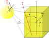 |
Fig. 1 Local Cartesian model. M is the origin of the set-up. The east, north and gravity (g) directions are along the x, y and z axis, respectively. The angle θ is the inclination of the rotation axis with respect to gravity. |
Next, we introduce the control parameters of the system:
-
the convective Rossby number definedas in Stevenson (1979)
 (3)where we introduce the dynamical time
  and we recall the definition of the characteristic convective turn-over time Pc = Lc/Vc;
  and
and  correspond to rapid and slow rotation regimes, respectively;
 -
the Ekman number
 (4)which compares the respective strength of the viscous force and of the Coriolis acceleration (see also Auclair Desrotour et al. 2015).
3.2. The new eddy-viscosity prescription
As in previous works, which do not take into account the action of rotation on convection (see Sect. 2), we assume that: i) we have a scale-separation between turbulent convective flows and tidal velocities and ii) the turbulent friction on this latter can be modelled through a viscous force involving an eddy-viscosity coefficient.
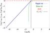 |
Fig. 2 Logarithm of the ratio νT;RC/νT;NR (and ERC/ENR) as a function of |
To derive this coefficient, we have to know the variation of Vc and Lc as a function of Ω and to verify that the mixing-length approach that is generally used in stellar and planetary models can be assumed in our context. Actually, in presence of (rapid) rotation, convective turbulence becomes highly anisotropic because of the action of the Coriolis acceleration (e.g. Julien et al. 2012; Sen et al. 2012; King et al. 2012, 2013) and one must verify that a simplified mixing-length approach can be assumed as a first step. In this framework, this is the great interest of the work by Barker et al. (2014). It demonstrated that scaling laws obtained for Vc and Lc as a function of  by Stevenson (1979) using such a mixing-length formalism is robust and verified when computing high-resolution Cartesian numerical simulations of rapidly rotating turbulent convective flows in a set-up corresponding to the one studied here.
We can thus generalize the prescription proposed in Eq. (2) to the rotating case by  (5)where RC stands for rotating convection. To get
  and
and  , we use the scaling laws that have been derived by Stevenson (1979) and verified by Barker et al. (2014) in the rapidly rotating regime:
-
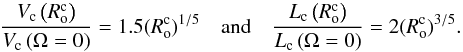
in the slow rotation regime, we have
 (6)and
 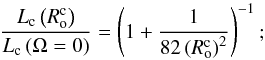 (7)
(7) -
in the rapid rotation regime, we have
 (8)
(8)
In Fig. 2, we plot log (νT;RC/νT;NR) and the corresponding ratio for the Ekman number (see Eq. (4)) as a function of  . We have defined a first Ekman number computed with the turbulent viscosity prescription where the modification of turbulent friction by rotation is ignored:
 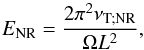 (9)and a second one where it is taken into account:
 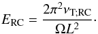 (10)In the regime of rapidly rotating convective flows (), the turbulent friction decreases by several orders of magnitude with a scaling
  . It can be understood by returning to the action of (rapid) rotation on the convective instability and turbulence (see the discussion at the end of Sect. 2). Indeed, the Coriolis acceleration tends to stabilize the flow and thus the degree of turbulence decreases with increasing rotation as well as the corresponding turbulent friction and eddy-viscosity.
Consequences for the viscous dissipation of the kinetic energy of tidal flows in rotating stellar and planetary convective regions must now be examined.
4. Consequences for tidal dissipation
4.1. A local model to quantify tidal dissipation
The linear response of planetary and stellar rotating convection zones to tidal perturbations is constituted by the superposition of an equilibrium/non-wave-like tide displacement and of tidally excited inertial waves, the dynamical tide (e.g. Zahn 1966; Ogilvie & Lin 2004, 2007; Remus et al. 2012; Ogilvie 2013). The restoring force of inertial waves is the Coriolis acceleration. Because of their dispersion relation σ = ± 2Ω kz/ | k |, where σ is their frequency and k their wave number, they propagate only if σ ∈ [−2Ω,2Ω].
To understand the impact of rapid rotation on the turbulent friction derived in the previous section on the equilibrium and dynamical tides, we now consider the linear response of the Cartesian set-up studied here (cf. Fig. 1) to a periodic tidal forcing. As a first step, we thus neglect the non-linear interactions between tidal inertial waves and those with turbulent convective flows (see, e.g. Galtier 2003; Sen et al. 2012; Favier et al. 2014; Clark di Leoni et al. 2014; Campagne et al. 2015). We follow the reduced and local analytical approach introduced by Ogilvie & Lin (2004) in the appendix of their paper and generalized by Auclair Desrotour et al. (2015) to understand tidal dissipation in convective regions with taking into account here the inclination angle θ. In this framework, the velocity field of the tide u excited by the tidal periodic volumetric forcing F per unit-mass is governed by the linearized momentum and continuity equations1:  (11)where ν is the (effective turbulent) viscosity and Π = P/ρ with P and ρ being the pressure and density respectively. We follow Ogilvie & Lin (2004) and Auclair Desrotour et al. (2015) by expanding u, Π, and f = F/ 2Ω as Fourier series in time and space
 ![Mathematical equation: \begin{eqnarray} \begin{array}{c c c} u_x = \Re \left[u(X,Z) {\rm e}^{-{\rm i} \omega T} \right], & u_y = \Re \left[v(X,Z) {\rm e}^{-{\rm i} \omega T} \right], \\[2mm] u_z = \Re \left[w(X,Z) {\rm e}^{-{\rm i} \omega T} \right], & \Pi = \Re \left[\psi (X,Z) {\rm e}^{-{\rm i} \omega T} \right], \\[2mm] f_x = \Re \left[f(X,Z) {\rm e}^{-{\rm i} \omega T} \right], & f_y = \Re \left[g (X,Z) {\rm e}^{-{\rm i} \omega T} \right], \\[2mm] f_z = \Re \left[h(X,Z) {\rm e}^{-{\rm i} \omega T} \right],\\ \end{array} \end{eqnarray}](/articles/aa/full_html/2016/08/aa27545-15/aa27545-15-eq60.png) (12)with
(12)with  (13)We have introduced the normalized space coordinates2X = x/L and Z = z/L, horizontal and vertical wave numbers m and n, time T = 2Ω t, and tidal frequency
  ;
;  is the mean orbital motion, s ∈ ZZZ and M = mL/ (rsinθ) = {1,2} (r is the radial spherical coordinate of M). The boundary conditions are periodic in the two directions that corresponds to normal modes excited by tides (e.g. Wu 2005; Braviner & Ogilvie 2015). It would be also possible to tackle the case of singular modes leading to inertial wave attractors by imposing rigid boundary conditions to our tilted Cartesian box (Ogilvie 2005; Jouve & Ogilvie 2014).
From the momentum and the continuity equations, we get the following system: ![Mathematical equation: \begin{equation} \left\{ \begin{array}{lcl} \!\! - {\rm i}\omega u_{mn} - \cos \theta v_{mn} + \sin \theta w_{mn} \!\!\!\!\! & = & \!\!\!\!\! - {\rm i} m \Lambda \psi_{mn} - E \left( m^2 + n^2 \right)u_{mn} + f_{mn}\\ \\[-1mm] - {\rm i}\omega v_{mn} + \cos \theta u_{mn} \!\!\!\!\! & = & \!\!\!\!\! - E \left( m^2 + n^2 \right)v_{mn} + g_{mn}\\ \vspace{1mm}\\ - {\rm i} \omega w_{mn} - \sin \theta u_{mn} \!\!\!\!\! & = & \!\!\!\!\! - {\rm i} n \Lambda \psi_{mn} - E \left( m^2 + n^2 \right)w_{mn} + h_{mn} \\ \\[-1mm] m u_{mn} + n w_{mn} \!\!\!\!\! & = & \!\!\!\!\! 0, \end{array} \right. \label{systeme_eq} \end{equation}](/articles/aa/full_html/2016/08/aa27545-15/aa27545-15-eq72.png) (14)where Λ = 1/(2Ω L). Following Auclair Desrotour et al. (2015), we solve it analytically. This allows us to derive each Fourier coefficient of the velocity field
(14)where Λ = 1/(2Ω L). Following Auclair Desrotour et al. (2015), we solve it analytically. This allows us to derive each Fourier coefficient of the velocity field ![Mathematical equation: \begin{equation} \left\{ \begin{array}{ccl} u_{mn} & = & \displaystyle n \frac{{\rm i} \tilde{\omega} \left( n f_{mn} - m h_{mn} \right) - n \cos \theta g_{mn} }{ \left( m^2 + n^2 \right) \tilde{\omega}^2 - n^2 \cos^2 \theta}\\ \\[-1.5mm] v_{mn} & = & \displaystyle\frac{n \cos \theta \left( n f_{mn} - m h_{mn} \right) + {\rm i} \left[\left( m^2 + n^2 \right) \tilde{\omega}\right] g_{mn} }{\left( m^2 + n^2 \right) \tilde{\omega}^2 - n^2 \cos^2 \theta}\\ \\[-1.5mm] w_{mn} & = & - m \displaystyle \frac{{\rm i} \tilde{\omega} \left( n f_{mn} - m h_{mn} \right) - n \cos \theta g_{mn} }{\left( m^2 + n^2 \right) \tilde{\omega}^2 - n^2 \cos^2 \theta}, \end{array} \right. \label{v:sol} \end{equation}](/articles/aa/full_html/2016/08/aa27545-15/aa27545-15-eq74.png) (15)with
(15)with 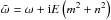 , and to compute the viscous dissipation per unit mass of the kinetic energy of tidal flows (Auclair Desrotour et al. 2015)
 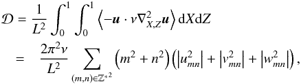 (16)where
  and ⟨···⟩ is the average in time, and the corresponding energy dissipated per rotation period
  (17)Because of the form of the forced velocity field (Eq. (15)), the tidal dissipation spectrum (ζ) is a complex resonant function of the normalized tidal frequency (ω). It corresponds to resonances of the inertial waves that propagate in planetary and stellar convection zones. An example of such resonant spectra is computed in Fig. 3 (top panel) for E = 10-4 and θ = 0. Here we use the academic forcing fmn = −i/(4 | m | n2), gmn = 0 and hmn = 0 adopted by Ogilvie & Lin (2004) and Auclair Desrotour et al. (2015). As discussed in Auclair Desrotour et al. (2015), such an academic forcing already allows us to study properly the variation of ζ as a function of rotation, viscosity and frequency forcing. Following this latter work, we characterize ζ by the following physical quantities and scaling laws in the local model:
-
the non-resonant background of the dissipation spectraHbg, which corresponds to the viscous dissipation of the equilibrium/non-wave-like tide, that scales as Hbg ∝ E;
-
the number of resonant peaks Nkc that scales as Nkc ∝ E− 1/2;
-
their width at half-height lmn that scales as lmn ∝ E;
-
their height Hmn that scales as Hmn ∝ E-1;
-
the sharpness of the spectrum defined as Ξ = H11/Hbg, which evaluate the contrast between the dissipation of the dynamical and equilibrium tides, that scales as Ξ ∝ E-2.
From now on, XRC is a quantity evaluated with ERC (i.e. with νT;RC) while XNR is computed using ENR (i.e. with νT;NR).
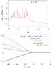 |
Fig. 3 Top: tidal dissipation frequency spectrum for the academic forcing chosen here (see also Ogilvie & Lin 2004; Auclair Desrotour et al. 2015) for E = 10-4 and θ = 0 (in logarithm scale for the dissipation). Bottom: variations of the logarithm of the ratios Hbg;RC/Hbg;NR, lRC/lNR (solid blue line), Nkc;RC/Nkc;NR (dashed purple line), HRC/HNR (dashed green line) and ΞRC/ ΞNR (long-dashed red line) as a function of |
4.2. The impact of rotation on the turbulent convective friction applied to tidal flows
We can thus deduce interesting conclusions from the results obtained with this simplified model for both the equilibrium and dynamical tides.
4.2.1. The equilibrium tide
In our local Cartesian set-up, the equilibrium tide is represented by the non-resonant background Hbg. Using Eq. (10), we thus deduce that its efficiency scales as Ω− 9/5 in the regime of rapid rotation. This loss of efficiency of the equilibrium tide in rapidly rotating convective regions is illustrated in Fig. 3 where we plot  as a function of .
4.2.2. The dynamical tide
We use scaling laws obtained for the resonances of tidal inertial waves. We deduce that as soon as studied convective regions are in the regime of rapid rotation, their number and height respectively increase as Nkc ∝ Ω9/10 and Hmn ∝ Ω9/5 while their width decreases as lmn ∝ Ω− 9/5. The sharpness of ζ is increased as Ξ ∝ Ω18/5. These variations of the properties of the resonant tidal dissipation frequency spectra is illustrated in Fig. 3 where we plot  ,
,  , and
, and  as a function of .
As demonstrated by Auclair-Desrotour et al. (2014; see also Witte & Savonije 1999), this may have important consequences for the evolution of the spin of the host body and of the orbits of the companions, for example in the cases of star-planet and planet-moon systems. Indeed, the relative migration induced by a resonance scales as  .
.
5. Astrophysical discussion
It is now important to discuss our results in the context of stellar and planetary interiors hosting turbulent convection regions. We focus here on the convective envelopes of low-mass stars (from M- to F-types) and of gaseous/icy giant planets and of the cores of telluric bodies.
5.1. The case of low-mass and solar-type stars
As demonstrated by Zahn (1966), Ogilvie & Lin (2007) and Mathis (2015), external convective zones of low-mass stars are key contributors for the dissipation of tidal kinetic energy in these objects3. This is illustrated by the observations of the state of the orbits and of stellar spins in planetary systems and binary stars (see the synthetic review in Ogilvie 2014, and references therein). An illustrative example is given by the need to understand the orbital properties of hot Jupiters and the inclination angle of their orbits relative to the spin axis of their host stars (e.g. Winn et al. 2010; Albrecht et al. 2012; Valsecchi & Rasio 2014b,a), which vary with their properties (i.e. their mass, age, rotation, etc.).
In this context, the rotation rates of low-mass stars strongly vary along their evolution (e.g. Barnes 2003; Gallet & Bouvier 2013, 2015; Amard et al. 2016; McQuillan et al. 2014; García et al. 2014). They are first locked in co-rotation with their initial circumstellar accretion disk because of complex MHD star-disk-wind interactions (e.g. Matt et al. 2010, 2012; Ferreira 2013). Next, because of their contraction, they spin up along the PMS until the zero-age main-sequence (ZAMS). Finally, they spin down during the MS because of the torque applied by magnetized stellar winds (e.g. Schatzman 1962; Kawaler 1988; Chaboyer et al. 1995; Réville et al. 2015; Matt et al. 2015). These variations of the angular velocity strongly affect the properties of convective flows because of the action of the Coriolis acceleration. Indeed, rapid rotation during the PMS modifies and constrains convective turbulent flow patterns, large-scale meridional circulations and differential rotation (Ballot et al. 2007; Brown et al. 2008). The key control parameters to unravel such a complex dynamic is the convective Rossby number defined in Eq. (3). For example, it allows us to predict the latitudinal behaviour of the differential rotation established by convection (Matt et al. 2011; Gastine et al. 2014; Käpylä et al. 2014) while it controls the friction applied to tidal flows (see Eq. (5)) and the properties of the frequency spectrum of their dissipation (see Sect. 4.2).
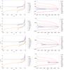 |
Fig. 4 Left-hand panels: radial profiles of |

It is thus interesting to compute the variations of along the evolution of low-mass stars. This will allow us to evaluate the impact of the action of rotation on the turbulent convective friction and on the properties of the tidal dissipation along stellar evolution thanks to Eqs. (5)−(8) and to scaling laws given in Sect. 4.1. To reach this objective, we choose to compute new grids of stellar rotating models for stars with masses between 0.6 M⊙ and 1.2 M⊙ (i.e. from K- to F-types) with a solar metallicity. We follow the methodology first proposed by Landin et al. (2010). This allows us to study the variations of the rotation and as a function of time and radius along the evolution of these stars from the beginning of the PMS to the end of the MS. We use the latest version of the STAREVOL stellar evolution code described in details (e.g. for the equation of state, nuclear reaction, opacities, etc.) in Amard et al. (2016; see also Siess et al. 2000; Palacios et al. 2003; Lagarde et al. 2012). The mixing-length parameter is chosen to be α = 1.6267. Convective regions are modelled assuming uniform rotation while radiation zones rotate according to redistribution of angular momentum by shear-induced turbulence and meridional flows, which are treated using formalisms derived by Zahn (1992), Maeder & Zahn (1998), Mathis & Zahn (2004), Mathis et al. (2004). Angular momentum losses at the stellar surface due to pressure-driven magnetized stellar winds are taken into account using the prescription adopted by Matt et al. (2015, the two parameters of this model are given in Eqs. (6) and (7) of this paper, and we choose χ = 10 and p = 2), which allows the authors to verify the Skumanich law (Skumanich 1972). Since our interest here is on the impact of rapid rotation, we choose to compute the evolution of initially rapidly rotating low-mass stars, which all have the same initial rotation period of 1.4 days and disc-locking time of 3 × 10⁶ yr. In addition, we have also computed the evolution of initially slow and median rotators that allows us to compare and validate our results with those obtained by Landin et al. (2010).
In Fig. 4 (left-hand panel), we first represent the radial profiles of for different masses (i.e. 0.6,0.8,1.0, and 1.2 M⊙) and ages: the beginning of the PMS, the mid PMS, the ZAMS, the middle of the MS, the end of the MS, and the solar age for the 1 M⊙ solar-type star4. In these plots (and in Fig. 5), we also recall the value of the critical convective Rossby number  . It corresponds to the transition between the rapidly (
 ) and slowly (
 ) rotating regimes. For all stellar masses and ages, a large radial variation of over several orders of magnitude is obtained with a monotonic increase towards the surface. This result is coherent with previously published results in the case of the Sun (see Fig. 1 in Käpylä et al. 2005). Therefore, the impact of rotation on the turbulent friction applied on tidal flows may be stronger close to the basis of the convective envelope than in surface regions. This may have different impacts on equilibrium and dynamical tides. On one hand, the equilibrium tide varies at the zeroth-order as
  , where
  is the quadrupolar spherical harmonics (see e.g. Zahn 1966; Remus et al. 2012). On the other hand, the dynamical tide constituted by tidal inertial waves propagate in the whole convective region. In the case of fully convective low-mass stars (at the beginning of the PMS or in M-type stars), inertial waves propagate as regular modes (Wu 2005). In the case of convective shells, they propagate along waves’ attractors (Ogilvie & Lin 2007). Therefore, for a given age, the turbulent friction applied on tidal inertial waves propagating deep inside convective zones would be more strongly affected by the action of the Coriolis acceleration on convective flows than the one applied on the equilibrium tide. However, for all stellar masses, we can see that the impact of rotation on the friction stays important everywhere during all the PMS and the beginning of the MS where stars are rotating rapidly. Indeed, during these evolution phases, the plotted radial profiles show that for all radii except just below the surface layers. This is confirmed in Fig. 5, where the convective Rossby number in the middle of the convective envelope (i.e. at r = ΔRCZ/ 2 = (Rs−Rc)/2, where Rs and Rc are the radius of the star and those of the basis of the convective envelope respectively) is plotted as a function of time. Indeed, Fig. 4 (left-hand panel) shows how
  can provide a reasonable intermediate order of magnitude for in tidal dissipation studies. At these evolutionary stages, we thus expect a strong action of the dynamical tide, constituted by inertial waves, with associated highly resonant tidal dissipation frequency-spectra. This result is very important since Zahn & Bouchet (1989) demonstrated that the most important phase of orbital circularization in late-type binaries occurs during the PMS where the convective envelopes of the components are thick. Moreover, it perfectly matches the results obtained by Mathis (2015) and Bolmont & Mathis (2016) where a strong action of tidal inertial waves all along the PMS has been identified. In Figs. 4 (right-hand panels) and 6, we represent the ratios between the values of the turbulent eddy-viscosity (and of the corresponding Ekman number) and those of the dissipation frequency spectrum properties (Hbg, l, H, Nkc and Ξ) (respectively as a function of r for {0.6,0.8,1,1.2} M⊙ stars at the middle of the PMS and MS in Fig. 4 (right-hand panels) and as a function of time for r = ΔRCZ/ 2 for stellar masses from 0.6 to 1.2 M⊙ in Fig. 6) when taking into account the modification of the turbulent friction by rotation or not. In each case, we see that differences by several orders of magnitude can be obtained for each quantity that must be taken into account. It demonstrates that the rapidly-rotating regime enhances the highly resonant dynamical tide while it decreases the efficiency of the equilibrium tide because the amplitudes of their viscous dissipation increases and decreases respectively with νT. Therefore, it strengthens the general conclusion that tidal evolution of star-planet systems and of binary stars must be treated taking into account the dynamical tide and not only the equilibrium tide (e.g. Auclair-Desrotour et al. 2014; Savonije & Witte 2002; Witte & Savonije 2002). As a consequence, the predictions obtained using simplified equilibrium tide models such as the constant tidal quality factor and the constant tidal lag models (e.g. Kaula 1964; Hut 1981) must be considered very carefully. As a conclusion, these results demonstrate how it is necessary to have an integrated and coupled treatment of the rotational evolution of stars, which directly impacts tidal dissipation in their interiors, and of the tidal evolution of the surrounding planetary or stellar systems (e.g. Penev et al. 2014; Bolmont & Mathis 2016). In addition, tidal torques may also modify the rotation of stars as a back reaction (e.g. Bolmont et al. 2012; Bolmont & Mathis 2016).
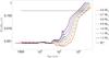 |
Fig. 5 Evolution of |
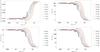 |
Fig. 6 Top left: evolution of νT;RC/νT;NR, ERC/ENR, Hbg;RC/Hbg;NR and lRC/lNR at r = ΔRCZ/ 2 (not written on labels to lighten notations) as a function of stellar age (in logarithm scales) for stellar masses from 0.6 M⊙ to 1.2 M⊙ (colours have been in defined in the caption of Fig. 5). Top right: same for HRC/HNR. Bottom left: same for NRC/NNR. Bottom right: same for ΞRC/ ΞNR. |
Finally, variations of ENR and ERC (with L = Rs; see Eqs. (9) and (10)) evaluated at r = ΔRCZ/ 2 as a function of stellar mass and age are given in Fig. 7 with f (in Eq. (5)) fixed to one, in left- and right-hand panels respectively. STAREVOL models allow us to coherently compute Vc, Lc and (Eq. (5)) for each stellar mass, age and radius. In these plots, we identify the phase of co-rotation of the stars with the surrounding disk (up to 3 × 10⁶ yr), the acceleration phase, and the stellar spin-down due to the breaking by the wind. This provides key inputs for future numerical simulations of tidal dissipation in spherical convective shells for which the Ekman number is one of the key physical control parameters (e.g. Ogilvie & Lin 2007; Baruteau & Rieutord 2013; Guenel et al. 2016). It allows us to improve step by step the evaluation of tidal friction in the convective envelope of low-mass stars all along their evolution by combining hydrodynamical studies and stellar modelling.
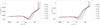 |
Fig. 7 Evolution of the Ekman numbers ENR (left panel) and ERC (right panel) at r = ΔRCZ/ 2 as a function of stellar age (in logarithm scales) for stellar masses from 0.6 M⊙ to 1.2 M⊙ (colours defined in the caption of Fig. 5). |
5.2. The case of planets
As in the case of young low-mass stars, convective flows are strongly constrained by the Coriolis acceleration in rapidly rotating planetary interiors. The most evident cases are those of the Earth liquid core and of the envelopes of gaseous (Jupiter and Saturn) and icy (Uranus and Neptune) giant planets (Glatzmaier 2013). In this context, the importance of rotation on tidal flows and their dissipation has been demonstrated both in the case of the Earth (e.g. Buffett 2010) and of giant planets (e.g. Ogilvie & Lin 2004; Wu 2005).
Therefore, as in the case of stars, it is interesting to collect values of the convective Rossby numbers for planetary interiors. We choose here to use the orders of magnitude given in Schubert & Soderlund (2011) for the Earth and in Soderlund et al. (2013) for giant planets. They are reported in the following table.
Orders of magnitude for planetary Rossby numbers (given in Schubert & Soderlund 2011, for the Earth, and in Soderlund et al. 2013, for giant planets).
From our previous results, we conclude that the rapidly-rotating regime (see Fig. 2) applies in the cases of the Earth, Jupiter, Saturn, Uranus and Neptune. Therefore, the action of the Coriolis acceleration on the convective turbulent friction cannot be neglected. It will strengthen the importance of tidal inertial waves and of their resonant viscous dissipation with corresponding numerous and strong resonances (see, e.g. Fig. 3). Note that such a result is particularly important for our understanding of tidal dissipation in the deep convective envelope of giant planets in our Solar System (Ogilvie & Lin 2004; Guenel et al. 2014) for which we obtained new constrains through high precision astrometry (Lainey et al. 2009, 2012, 2015).
We can thus conclude that in most of the astrophysical situations relevant for the evolution of planetary systems, the action of rotation on the turbulent friction applied by convection on linear tidal waves must be taken into account. Moreover, it demonstrates that it is necessary to build a coupled modelling of the tidal evolution of planetary systems with the rotational evolution of their components, rotation being a key parameter for the amplitude and the frequency dependence of tidal dissipation in their interiors.
6. Conclusions and perspectives
Using results obtained by Barker et al. (2014) on the scaling of velocities and length scales in rotating turbulent convection zones, we proposed a new prescription for the eddy-viscosity coefficient, which allows us to describe tidal friction in such regions. In their work, Barker et al. (2014) confirmed scalings for convective velocities and length scales as a function of rotation in the rapidly rotating regime that were first derived by Stevenson (1979) using mixing-length theory. Using his results, we derive a new prescription for the turbulent friction, which takes into account the action of the Coriolis acceleration on the convective flows. This allows us to generalize previous studies where the action of rotation on linear tidal flows was accounted for while its impact on the turbulent friction applied on them by convection was ignored. We demonstrated that the eddy-viscosity may be decreased by several orders of magnitude in the rapidly rotating regime. It leads to a deep modification of the tidal dissipation frequency spectrum. On one hand, its background that corresponds to the so-called equilibrium/non-wave-like tide is decreased because it scales as E ∝ νT. On the other hand, resonances of tidal inertial waves (i.e. the dynamical tide) become more and more numerous, higher and sharper since their number, width at half-height, height, and sharpness respectively scales as E− 1/2, E, E-1, and E-2 (Auclair Desrotour et al. 2015). In this framework, we demonstrated using new grids of rotating low-mass stars and values of convective Rossby numbers in planetary interiors (Schubert & Soderlund 2011; Soderlund et al. 2013), that this modification of the turbulent friction is important for low-mass stars along their PMS and at the beginning of MS during which they are rapidly rotating and in rapidly rotating planets as the Earth and giant gaseous/icy planets. Because of the radial variation of the effects of rotation on the friction, they may be stronger for tidal inertial waves that propagate in the whole convective zone than for the equilibrium tide which has a higher amplitude in surface regions. As demonstrated by Auclair-Desrotour et al. (2014), such a behaviour must be taken into account in the study of the tidal evolution of star-planet and planet-moon systems. Indeed, the angular velocity of their components vary through time because of structural modifications and of applied (tidal and electromagnetic) torques. These torques are themselves complex functions of rotation (this work; Mathis 2015; Matt et al. 2012, 2015; Réville et al. 2015). It is thus necessary to have a completely coupled treatment of the tidal evolution of planetary systems and multiple stars and of the rotational evolution of their components with a coherent treatment of the variations of tidal flows and of their dissipation as a function of rotation.
In our work, the non-linear wave-wave interactions and those between tidal and convective flows have been ignored (e.g. Sen et al. 2012; Sen 2013; Barker & Lithwick 2013; Favier et al. 2014). Moreover, stratified convection, with intermediate stably stratified diffusive layers can take place in giant planets because of double-diffusive instabilities (Leconte & Chabrier 2012). Finally, stellar and planetary convective regions are differentially rotating and magnetized (Baruteau & Rieutord 2013; Guenel et al. 2016; Barker & Lithwick 2014). In the near future, these four aspects of the problem will be examined carefully to improve our knowledge of tidal friction in stars and planets.
In this work the action of thermal diffusivity is ignored.
As in Ogilvie & Lin (2004) and Auclair Desrotour et al. (2015), we focus on solutions, which depend only on X and Z, since adding the third coordinate Y will not modify the qualitative behaviour of the system.
Zahn (1977) showed that tidal dissipation in intermediate-mass and massive stars is dominated by thermal diffusion acting on gravity waves in their radiative envelope.
Note here that we consider a 1 M⊙ solar-type star and not a helioseismic calibrated solar model.
Acknowledgments
The authors thank the referee for his positive and constructive report which allowed us to improve the article. The authors acknowledge funding by the European Research Council through ERC grant SPIRE 647383. This work was also supported by the Programme National de Planétologie (CNRS/INSU), the GRAM specific action (CNRS/INSU-INP, CNES), the Axe Etoile of the Paris Observatory Scientific Council and the International Space Institute (ISSI team ENCELADE 2.0). We dedicate this article to our friend Pr. André Brahic who was continuously promoting research, culture and education and to his values “Courage, Liberté, Egalité, Fraternité”.
References
- Albrecht, S., Winn, J. N., Johnson, J. A., et al. 2012, ApJ, 757, 18 [NASA ADS] [CrossRef] [Google Scholar]
- Amard, L., Palacios, A., Charbonnel, C., Gallet, F., & Bouvier, J. 2016, A&A, 587, A105 [NASA ADS] [CrossRef] [EDP Sciences] [Google Scholar]
- Auclair-Desrotour, P., Le Poncin-Lafitte, C., & Mathis, S. 2014, A&A, 561, L7 [NASA ADS] [CrossRef] [EDP Sciences] [Google Scholar]
- Auclair Desrotour, P., Mathis, S., & Le Poncin-Lafitte, C. 2015, A&A, 581, A118 [NASA ADS] [CrossRef] [EDP Sciences] [Google Scholar]
- Ballot, J., Brun, A. S., & Turck-Chièze, S. 2007, ApJ, 669, 1190 [Google Scholar]
- Barker, A. J., & Lithwick, Y. 2013, MNRAS, 435, 3614 [NASA ADS] [CrossRef] [Google Scholar]
- Barker, A. J., & Lithwick, Y. 2014, MNRAS, 437, 305 [NASA ADS] [CrossRef] [Google Scholar]
- Barker, A. J., Dempsey, A. M., & Lithwick, Y. 2014, ApJ, 791, 13 [NASA ADS] [CrossRef] [Google Scholar]
- Barnes, S. A. 2003, ApJ, 586, 464 [NASA ADS] [CrossRef] [Google Scholar]
- Baruteau, C., & Rieutord, M. 2013, J. Fluid Mechanics, 719, 47 [NASA ADS] [CrossRef] [Google Scholar]
- Bolmont, E., & Mathis, S. 2016, Celest. Mech. Dyn. Astron., in press [arXiv:1603.06268] [Google Scholar]
- Bolmont, E., Raymond, S. N., Leconte, J., & Matt, S. P. 2012, A&A, 544, A124 [NASA ADS] [CrossRef] [EDP Sciences] [Google Scholar]
- Bouvier, J. 2008, A&A, 489, L53 [NASA ADS] [CrossRef] [EDP Sciences] [Google Scholar]
- Braviner, H. J., & Ogilvie, G. I. 2015, MNRAS, 447, 1141 [NASA ADS] [CrossRef] [Google Scholar]
- Brown, B. P., Browning, M. K., Brun, A. S., Miesch, M. S., & Toomre, J. 2008, ApJ, 689, 1354 [CrossRef] [Google Scholar]
- Brun, A. S. 2014, in IAU Symp. 302, eds. P. Petit, M. Jardine, & H. C. Spruit, 114 [Google Scholar]
- Buffett, B. 2010, Nature, 468, 952 [NASA ADS] [CrossRef] [Google Scholar]
- Campagne, A., Gallet, B., Moisy, F., & Cortet, P.-P. 2015, Phys. Rev. E, 91, 043016 [NASA ADS] [CrossRef] [Google Scholar]
- Chaboyer, B., Demarque, P., & Pinsonneault, M. H. 1995, ApJ, 441, 865 [NASA ADS] [CrossRef] [Google Scholar]
- Chandrasekhar, S. 1953, R. Soc. Lond. Proc. Ser. A, 217, 306 [Google Scholar]
- Clark di Leoni, P., Cobelli, P. J., Mininni, P. D., Dmitruk, P., & Matthaeus, W. H. 2014, Phys. Fluids, 26, 035106 [NASA ADS] [CrossRef] [Google Scholar]
- Efroimsky, M., & Lainey, V. 2007, J. Geophys. Res., 112, 12003 [Google Scholar]
- Favier, B., Barker, A. J., Baruteau, C., & Ogilvie, G. I. 2014, MNRAS, 439, 845 [NASA ADS] [CrossRef] [Google Scholar]
- Ferreira, J. 2013, in EAS Pub. Ser. 62, eds. P. Hennebelle & C. Charbonnel, 169 [Google Scholar]
- Gallet, F., & Bouvier, J. 2013, A&A, 556, A36 [NASA ADS] [CrossRef] [EDP Sciences] [Google Scholar]
- Gallet, F., & Bouvier, J. 2015, A&A, 577, A98 [NASA ADS] [CrossRef] [EDP Sciences] [Google Scholar]
- Galtier, S. 2003, Phys. Rev. E, 68, 015301 [NASA ADS] [CrossRef] [Google Scholar]
- García, R. A., Ceillier, T., Salabert, D., et al. 2014, A&A, 572, A34 [NASA ADS] [CrossRef] [EDP Sciences] [Google Scholar]
- Gastine, T., Yadav, R. K., Morin, J., Reiners, A., & Wicht, J. 2014, MNRAS, 438, L76 [NASA ADS] [CrossRef] [Google Scholar]
- Glatzmaier, G. A. 2013, Introduction to Modelling Convection in Planets and Stars (Princeton University Press) [Google Scholar]
- Goldreich, P., & Keeley, D. A. 1977, ApJ, 211, 934 [NASA ADS] [CrossRef] [Google Scholar]
- Goldreich, P., & Soter, S. 1966, Icarus, 5, 375 [NASA ADS] [CrossRef] [Google Scholar]
- Goodman, J., & Oh, S. P. 1997, ApJ, 486, 403 [NASA ADS] [CrossRef] [Google Scholar]
- Guenel, M., Mathis, S., & Remus, F. 2014, A&A, 566, L9 [NASA ADS] [CrossRef] [EDP Sciences] [Google Scholar]
- Guenel, M., Baruteau, C., Mathis, S., & Rieutord, M. 2016, A&A, 589, A22 [NASA ADS] [CrossRef] [EDP Sciences] [Google Scholar]
- Hut, P. 1981, A&A, 99, 126 [NASA ADS] [Google Scholar]
- Jouve, L., & Ogilvie, G. I. 2014, J. Fluid Mech., 745, 223 [Google Scholar]
- Julien, K., Knobloch, E., Rubio, A. M., & Vasil, G. M. 2012, Phys. Rev. Lett., 109, 254503 [NASA ADS] [CrossRef] [Google Scholar]
- Käpylä, P. J., Korpi, M. J., Stix, M., & Tuominen, I. 2005, A&A, 438, 403 [NASA ADS] [CrossRef] [EDP Sciences] [Google Scholar]
- Käpylä, P. J., Käpylä, M. J., & Brandenburg, A. 2014, A&A, 570, A43 [NASA ADS] [CrossRef] [EDP Sciences] [Google Scholar]
- Kaula, W. M. 1964, Rev. Geophys. Space Phys., 2, 661 [Google Scholar]
- Kawaler, S. D. 1988, ApJ, 333, 236 [NASA ADS] [CrossRef] [Google Scholar]
- King, E. M., Stellmach, S., & Aurnou, J. M. 2012, J. Fluid Mech., 691, 568 [NASA ADS] [CrossRef] [Google Scholar]
- King, E. M., Stellmach, S., & Buffett, B. 2013, J. Fluid Mech., 717, 449 [NASA ADS] [CrossRef] [Google Scholar]
- Lagarde, N., Decressin, T., Charbonnel, C., et al. 2012, A&A, 543, A108 [NASA ADS] [CrossRef] [EDP Sciences] [Google Scholar]
- Lainey, V., Arlot, J.-E., Karatekin, Ö., & van Hoolst, T. 2009, Nature, 459, 957 [NASA ADS] [CrossRef] [PubMed] [Google Scholar]
- Lainey, V., Karatekin, Ö., Desmars, J., et al. 2012, ApJ, 752, 14 [NASA ADS] [CrossRef] [Google Scholar]
- Lainey, V., Jacobson, R. A., Tajeddine, R., et al. 2015, ArXiv e-prints [arXiv:1510.05870] [Google Scholar]
- Landin, N. R., Mendes, L. T. S., & Vaz, L. P. R. 2010, A&A, 510, A46 [NASA ADS] [CrossRef] [EDP Sciences] [Google Scholar]
- Laskar, J., Boué, G., & Correia, A. C. M. 2012, A&A, 538, A105 [NASA ADS] [CrossRef] [EDP Sciences] [Google Scholar]
- Leconte, J., & Chabrier, G. 2012, A&A, 540, A20 [NASA ADS] [CrossRef] [EDP Sciences] [Google Scholar]
- Maeder, A., & Zahn, J.-P. 1998, A&A, 334, 1000 [NASA ADS] [Google Scholar]
- Mathis, S. 2015, A&A, 580, L3 [Google Scholar]
- Mathis, S., & Remus, F. 2013, in Lect. Not. Phys. 857 (Berlin: Springer Verlag), eds. J.-P. Rozelot, & C. Neiner, 111 [Google Scholar]
- Mathis, S., & Zahn, J.-P. 2004, A&A, 425, 229 [NASA ADS] [CrossRef] [EDP Sciences] [Google Scholar]
- Mathis, S., Palacios, A., & Zahn, J.-P. 2004, A&A, 425, 243 [NASA ADS] [CrossRef] [EDP Sciences] [Google Scholar]
- Matt, S. P., Pinzón, G., de la Reza, R., & Greene, T. P. 2010, ApJ, 714, 989 [NASA ADS] [CrossRef] [Google Scholar]
- Matt, S. P., Do Cao, O., Brown, B. P., & Brun, A. S. 2011, Astron. Nachr., 332, 897 [NASA ADS] [CrossRef] [Google Scholar]
- Matt, S. P., Pinzón, G., Greene, T. P., & Pudritz, R. E. 2012, ApJ, 745, 101 [NASA ADS] [CrossRef] [Google Scholar]
- Matt, S. P., Brun, A. S., Baraffe, I., Bouvier, J., & Chabrier, G. 2015, ApJ, 799, L23 [NASA ADS] [CrossRef] [Google Scholar]
- McQuillan, A., Mazeh, T., & Aigrain, S. 2014, ApJS, 211, 24 [NASA ADS] [CrossRef] [MathSciNet] [Google Scholar]
- Ogilvie, G. I. 2005, J. Fluid Mech., 543, 19 [NASA ADS] [CrossRef] [Google Scholar]
- Ogilvie, G. I. 2013, MNRAS, 429, 613 [NASA ADS] [CrossRef] [Google Scholar]
- Ogilvie, G. I. 2014, ARA&A, 52, 171 [Google Scholar]
- Ogilvie, G. I., & Lesur, G. 2012, MNRAS, 422, 1975 [NASA ADS] [CrossRef] [Google Scholar]
- Ogilvie, G. I., & Lin, D. N. C. 2004, ApJ, 610, 477 [NASA ADS] [CrossRef] [Google Scholar]
- Ogilvie, G. I., & Lin, D. N. C. 2007, ApJ, 661, 1180 [NASA ADS] [CrossRef] [Google Scholar]
- Palacios, A., Talon, S., Charbonnel, C., & Forestini, M. 2003, A&A, 399, 603 [NASA ADS] [CrossRef] [EDP Sciences] [Google Scholar]
- Penev, K., Sasselov, D., Robinson, F., & Demarque, P. 2007, ApJ, 655, 1166 [NASA ADS] [CrossRef] [Google Scholar]
- Penev, K., Zhang, M., & Jackson, B. 2014, PASP, 126, 553 [NASA ADS] [CrossRef] [Google Scholar]
- Remus, F., Mathis, S., & Zahn, J.-P. 2012, A&A, 544, A132 [NASA ADS] [CrossRef] [EDP Sciences] [Google Scholar]
- Réville, V., Brun, A. S., Matt, S. P., Strugarek, A., & Pinto, R. F. 2015, ApJ, 798, 116 [NASA ADS] [CrossRef] [Google Scholar]
- Savonije, G. J., & Witte, M. G. 2002, A&A, 386, 211 [NASA ADS] [CrossRef] [EDP Sciences] [Google Scholar]
- Schatzman, E. 1962, Ann. Astrophys., 25, 18 [Google Scholar]
- Schubert, G., & Soderlund, K. M. 2011, Phys. Earth Planet. Interiors, 187, 92 [NASA ADS] [CrossRef] [Google Scholar]
- Sen, A. 2013, ArXiv e-prints [arXiv:1312.7497] [Google Scholar]
- Sen, A., Mininni, P. D., Rosenberg, D., & Pouquet, A. 2012, Phys. Rev. E, 86, 036319 [NASA ADS] [CrossRef] [Google Scholar]
- Siess, L., Dufour, E., & Forestini, M. 2000, A&A, 358, 593 [Google Scholar]
- Skumanich, A. 1972, ApJ, 171, 565 [NASA ADS] [CrossRef] [Google Scholar]
- Soderlund, K. M., Heimpel, M. H., King, E. M., & Aurnou, J. M. 2013, Icarus, 224, 97 [NASA ADS] [CrossRef] [Google Scholar]
- Stevenson, D. J. 1979, Geophys. Astrophys. Fluid Dyn., 12, 139 [NASA ADS] [CrossRef] [Google Scholar]
- Valsecchi, F., & Rasio, F. A. 2014a, ApJ, 787, L9 [NASA ADS] [CrossRef] [Google Scholar]
- Valsecchi, F., & Rasio, F. A. 2014b, ApJ, 786, 102 [NASA ADS] [CrossRef] [Google Scholar]
- Winn, J. N., Fabrycky, D., Albrecht, S., & Johnson, J. A. 2010, ApJ, 718, L145 [NASA ADS] [CrossRef] [Google Scholar]
- Witte, M. G., & Savonije, G. J. 1999, A&A, 350, 129 [NASA ADS] [Google Scholar]
- Witte, M. G., & Savonije, G. J. 2002, A&A, 386, 222 [NASA ADS] [CrossRef] [EDP Sciences] [Google Scholar]
- Wu, Y. 2005, ApJ, 635, 688 [NASA ADS] [CrossRef] [Google Scholar]
- Zahn, J. P. 1966, Ann. Astrophys., 29, 489 [NASA ADS] [Google Scholar]
- Zahn, J.-P. 1975, A&A, 41, 329 [NASA ADS] [Google Scholar]
- Zahn, J.-P. 1977, A&A, 57, 383 [NASA ADS] [Google Scholar]
- Zahn, J.-P. 1989, A&A, 220, 112 [NASA ADS] [Google Scholar]
- Zahn, J.-P. 1992, A&A, 265, 115 [NASA ADS] [Google Scholar]
- Zahn, J.-P., & Bouchet, L. 1989, A&A, 223, 112 [Google Scholar]
All Tables
Orders of magnitude for planetary Rossby numbers (given in Schubert & Soderlund 2011, for the Earth, and in Soderlund et al. 2013, for giant planets).
All Figures
|
Fig. 1 Local Cartesian model. M is the origin of the set-up. The east, north and gravity (g) directions are along the x, y and z axis, respectively. The angle θ is the inclination of the rotation axis with respect to gravity. |
| In the text | |
|
Fig. 2 Logarithm of the ratio νT;RC/νT;NR (and ERC/ENR) as a function of |
| In the text | |
|
Fig. 3 Top: tidal dissipation frequency spectrum for the academic forcing chosen here (see also Ogilvie & Lin 2004; Auclair Desrotour et al. 2015) for E = 10-4 and θ = 0 (in logarithm scale for the dissipation). Bottom: variations of the logarithm of the ratios Hbg;RC/Hbg;NR, lRC/lNR (solid blue line), Nkc;RC/Nkc;NR (dashed purple line), HRC/HNR (dashed green line) and ΞRC/ ΞNR (long-dashed red line) as a function of |
| In the text | |
|
Fig. 4 Left-hand panels: radial profiles of |
| In the text | |
|
Fig. 5 Evolution of |
| In the text | |
|
Fig. 6 Top left: evolution of νT;RC/νT;NR, ERC/ENR, Hbg;RC/Hbg;NR and lRC/lNR at r = ΔRCZ/ 2 (not written on labels to lighten notations) as a function of stellar age (in logarithm scales) for stellar masses from 0.6 M⊙ to 1.2 M⊙ (colours have been in defined in the caption of Fig. 5). Top right: same for HRC/HNR. Bottom left: same for NRC/NNR. Bottom right: same for ΞRC/ ΞNR. |
| In the text | |
|
Fig. 7 Evolution of the Ekman numbers ENR (left panel) and ERC (right panel) at r = ΔRCZ/ 2 as a function of stellar age (in logarithm scales) for stellar masses from 0.6 M⊙ to 1.2 M⊙ (colours defined in the caption of Fig. 5). |
| In the text | |
Current usage metrics show cumulative count of Article Views (full-text article views including HTML views, PDF and ePub downloads, according to the available data) and Abstracts Views on Vision4Press platform.
Data correspond to usage on the plateform after 2015. The current usage metrics is available 48-96 hours after online publication and is updated daily on week days.
Initial download of the metrics may take a while.