| Issue |
A&A
Volume 591, July 2016
|
|
|---|---|---|
| Article Number | A124 | |
| Number of page(s) | 15 | |
| Section | Stellar structure and evolution | |
| DOI | https://doi.org/10.1051/0004-6361/201628581 | |
| Published online | 24 June 2016 | |
Absolute parameters for AI Phoenicis using WASP photometry
1
Astrophysics Group, Keele University, Keele, Staffordshire
ST5 5BG, UK
e-mail: This email address is being protected from spambots. You need JavaScript enabled to view it.
2
Institute of Space Sciences (ICE/CSIC-IEEC),
Carrer de Can Magrans S/N,
08193
Cerdanyola del Valles,
Spain
3
Department of Physics, University of Warwick,
Coventry, CV4 7AL, UK
Received: 23 March 2016
Accepted: 21 May 2016
Abstract
Context. AI Phe is a double-lined, detached eclipsing binary, in which a K-type sub-giant star totally eclipses its main-sequence companion every 24.6 days. This configuration makes AI Phe ideal for testing stellar evolutionary models. Difficulties in obtaining a complete lightcurve mean the precision of existing radii measurements could be improved.
Aims. Our aim is to improve the precision of the radius measurements for the stars in AI Phe using high-precision photometry from the Wide Angle Search for Planets (WASP), and use these improved radius measurements together with estimates of the masses, temperatures and composition of the stars to place constraints on the mixing length, helium abundance and age of the system.
Methods. A best-fit ebop model is used to obtain lightcurve parameters, with their standard errors calculated using a prayer-bead algorithm. These were combined with previously published spectroscopic orbit results, to obtain masses and radii. A Bayesian method is used to estimate the age of the system for model grids with different mixing lengths and helium abundances.
Results. The radii are found to be R1 = 1.835 ± 0.014 R⊙, R2 = 2.912 ± 0.014 R⊙ and the masses M1 = 1.1973 ± 0.0037 M⊙, M2 = 1.2473 ± 0.0039 M⊙. From the best-fit stellar models we infer a mixing length of 1.78, a helium abundance of YAI = 0.26 +0.02-0.01 and an age of 4.39 ± 0.32 Gyr. Times of primary minimum show the period of AI Phe is not constant. Currently, there are insufficient data to determine the cause of this variation.
Conclusions. Improved precision in the masses and radii have improved the age estimate, and allowed the mixing length and helium abundance to be constrained. The eccentricity is now the largest source of uncertainty in calculating the masses. Further work is needed to characterise the orbit of AI Phe. Obtaining more binaries with parameters measured to a similar level of precision would allow us to test for relationships between helium abundance and mixing length.
Key words: stars: solar-type / stars: evolution / stars: fundamental parameters / binaries: eclipsing
© ESO, 2016
1. Introduction
Stellar evolutionary models are used in a variety of areas of astrophysics, from predicting the properties of stars in galaxy formation models (Schaerer 2013), to characterising planetary host stars (Boyajian et al. 2015; Cabrera et al. 2015). However, there are an increasing number of cases where the models have failed to reproduce the observed parameters of low-mass stars within binary systems. For example, observations of IM Vir (a G7+K7-type binary) found the radii of the primary and secondary components were larger than those predicted by the models by 3.7% and 7.5%, respectively (Morales et al. 2009), while the temperatures of the primary and secondary were found to be 100 K and 150 K (respectively) cooler than model predictions. Vos et al. (2012) showed the secondary of EF Aqr (a G0-type system) is 9% larger and 400 K cooler than model predictions. A similar situation was found for V530 Ori (a G1+M1-type binary), for which models predicted a radius 3.7% smaller than observations and a temperature that was 4.8% hotter than observations (Torres et al. 2014). The problems with the models are not unique to stars within binary systems. A study of 183 low-mass K7-M7 single stars by Mann et al. (2015) using an inferred stellar mass, found that models over-predicted the effective temperature (Teff) by 2.2% and under-predict radii by 4.6%. In some cases, magnetic fields have been used to explain the discrepancies, e.g. V530 Ori (Torres et al. 2014), but it remains unclear whether magnetic fields provide the solution in all cases (Mann et al. 2015). For low-mass stars, explanations for the discrepancies are discussed by Torres (2013), where they conclude that systems with well-determined masses, radii, temperatures and metallicities, will be important in trying to understand this problem.
AI Phoenicis (AI Phe, HD 6980) is one of a number of important eclipsing binary systems within astrophysics. Many other subgiant systems exhibit flares or spots that are associated with the strong magnetic activity of RS CVn systems. However, due its long period and slow rotation, AI Phe does not display any of these photometric complications (Andersen et al. 1988). This makes it possible to obtain high-precision masses and radii for the system, and treat the components as independent stars for modelling purposes. Its specific combination of a main-sequence star and a sub-giant star make it ideal for testing stellar evolutionary models. This was demonstrated by Torres et al. (2010) using two different codes to model the system (Yonsei-Yale and an experimental version of the Victoria models). They aimed to reproduce the radii and effective temperatures at an age that was consistent for both components, and found the mean age of the system is different by 0.9 Gyr between the two models. This is a non-negligible uncertainty when determining the ages of nearby solar-type stars. Spada et al. (2013) also used AI Phe to test their evolutionary code by attempting to produce tracks for each component that give consistent ages for both components. They found an age of 4.44 Gyr for the hotter component and 4.54 Gyr for the cooler component, with agreement at the 2% level. The treatment of convective-core overshooting, mixing-length and helium abundance can be significant sources of uncertainty within the models (Lebreton et al. 2014). With high precision masses and radii for a binary such as AI Phe, the age of the system can be tightly constrained, as the number of plausible evolutionary tracks is greatly reduced. It therefore provides an excellent opportunity to get a better understanding of overshooting, the helium abundance and mixing length parameter.
AI Phe was first noted as an eclipsing binary by Strohmeier (1972). Photometric analysis to obtain the first accurate estimate of the orbital period was carried out by Reipurth (1978). Imbert (1979) carried out the first spectroscopic analysis of the orbit. Hrivnak & Milone (1984) used the spectroscopic orbit data of Imbert (1979), together with new photometric observations in UBVRI, to obtain masses and radii for AI Phe. Vandenberg & Hrivnak (1985) compared the observed parameters of AI Phe to theoretical isochrones to calculate the helium abundance, Y, and age, τ, of the system (Y = 0.38 ± 0.05 and τ = 3.6 ± 0.7 Gyr). Andersen et al. (1988) used new radial velocity (RV) measurements, the UBVRI photometric data of Hrivnak & Milone (1984) and new uvby photometry to obtain masses to ±0.3% and radii to ±1.5%. At the time, these were most accurately determined masses for any detached, double-lined eclipsing binary system (Andersen 1991). Milone et al. (1992) remodelled the data of Andersen et al. (1988) and Hrivnak & Milone (1984), using Wilson-Devinney code with updated model atmospheres. Their work reduced the uncertainties on the radii, although their value for the secondary component was 2σ lower than the value found by Andersen et al. (1988). Karami & Mohebi (2007) reanalysed the RV data of Andersen et al. (1988) using a nonlinear regression method, which allowed semi-amplitude velocity, eccentricity and longitude of periastron to be fitted simultaneously. However, Hełminiak et al. (2009) suggested that the errors quoted by Karami & Mohebi were underestimated due to several uncertainties not being included in their error analysis. Hełminiak et al. (2009) used new spectra to obtain RV measurements with a root mean squared (RMS) residuals from the spectroscopic orbit fit of 62 and 24 m s-1 for the primary and secondary components, respectively. They also used photometric data from All-Sky Automated Survey (ASAS, Pojmanski 2002) to obtain masses and radii for the components, but noted that they only had access to one lightcurve for their work, and suggested the derived parameters of AI Phe could be improved further with high-precision photometry.
The SuperWASP cameras monitor thousands of stars every night looking for planetary transits, as part of the Wide Angle Search for Planets (WASP, Pollacco et al. 2006). WASP also provides an excellent opportunity to find and study eclipsing binary systems using photometry with better than 1% accuracy. This paper focuses on the analysis WASP photometry to derive high precision lightcurve parameters for AI Phe. These are then combined with the RV measurements of Hełminiak et al. (2009) to obtain radii to a precision of better than 1%. Section 2 provides a description of the photometric data used for the work. Section 3 describes the data processing, lightcurve modelling, and error analysis. Section 4 contains a summary of the final masses and radii, while Sect. 5 uses the new masses and radii as constraints to determine the age of the system using models different mixing lengths and helium abundance. Finally, Sects. 6 and 7 contain a discussion of the results and conclusion, respectively.
2. Data
2.1. Observations
Located at the Observatorio del Roque de los Muchachos, La Palma and at Sutherland Observatory, South Africa, the two WASP instruments are both formed from eight wide-field cameras each with a 2048 × 2048 pixel CCD. For AI Phe (1SWASP J010934.19-461556.0), over 170 000 photometric measurements were present in the WASP archive, taken between June 2006 and January 2014 by the instrument in South Africa. During this period, WASP-South has used two different types of lenses, the original 200-mm, f/1.8 lenses (Pollacco et al. 2006) and, from July 2012, 85-mm, f/1.2 lenses (Smith & WASP Consortium 2014). The reduction procedure is identical for both lens types, and uses a dedicated pipeline (Pollacco et al. 2006) that has been optimised in each case. The data are then processed by a detrending algorithm, which was developed from the SysRem algorithm of Tamuz et al. (2005) and is described by Collier Cameron et al. (2006).
Use of the 85-mm lenses allows WASP-South to focus on brighter stars (V ≲ 9). A larger reduction aperture is used in comparison to the 200-mm lenses (4 pixels from 3.5) and the limits on image and star rejection were also modified. This results in a shift of the photometry range to 6 ≲ V ≲ 11 for the 85-mm lenses from 9 ≲ V ≲ 13 for the 200-mm lenses. The 200-mm lenses use broad-band filters with a range of 400−700 nm, while the 85-mm use SDSS r′ filters. Observations from the two different types of lens have been analysed separately.
2.2. Initial processing
The WASP data can suffer from large amounts of scatter, due to clouds, etc. This section describes the methods used to remove unreliable observations in the two sets of data.
For the 200-mm data, a decision was made to only use data from cameras 225 and 226 during the analysis. These two cameras contribute more than 80% of the observations made with the 200-mm cameras. The data from the other cameras contained large amounts of scatter, perhaps related to the fact that the 200-mm lenses are very close to their saturation limit for AI Phe. They also only contributed a handful of observations to the eclipses, and would not help determine the radii of AI Phe.
As part of the WASP reduction pipeline, each photometric measurement gets assigned a weighting factor, σxs, (denoted σt(i) in Collier Cameron et al. 2006), to characterise the scatter present from external noise sources. This σxs value is set to zero if the pipeline deems the value to be missing or bad (Collier Cameron et al. 2006), so data with σxs = 0 were not included in any analysis. In some cases, the error in the measured flux was exceptionally high in comparison with the other measurements. It is likely that this is due to clouds being present at the time of exposure, as σxs is also higher for these data. If the error in a particular flux measurement was five or more times greater than the median error of all data from the same camera, then it was excluded from our analysis.
The flux measurement we have used for our analysis, f, is calculated from an
aperture with a radius of 3.5 pixels or 4 pixels (for the 200-mm and 85-mm lenses,
respectively) centred on AI Phe, with the detrending correction of Collier Cameron et al. (2006) applied, and ferr is the
associated error in this value. The magnitude of each measurement was calculated from
f using the
median flux of the data set as the zero point. The error in magnitude, merr, associated
with each observation, was calculated using  (1)One final check was used to look for sections
of data that were significantly offset from the remaining data. The phase-folded data was
split into 800 phase bins. The median magnitude and associated error in the median were
then calculated for each bin. This formed a model from which we could estimate the
expected magnitude of an observation given its phase. The entire data set was also split
into blocks based on the night the observation was taken and the camera used. For each
data block, the magnitude of each observation within that block was compared to its
expected magnitude by matching it to a phase bin. If more than 80% of the observations
from a particular data block were offset by more than ten times the errors associated with
the appropriate phase-bins, then all data from that night/camera combination were excluded
from the analysis.
(1)One final check was used to look for sections
of data that were significantly offset from the remaining data. The phase-folded data was
split into 800 phase bins. The median magnitude and associated error in the median were
then calculated for each bin. This formed a model from which we could estimate the
expected magnitude of an observation given its phase. The entire data set was also split
into blocks based on the night the observation was taken and the camera used. For each
data block, the magnitude of each observation within that block was compared to its
expected magnitude by matching it to a phase bin. If more than 80% of the observations
from a particular data block were offset by more than ten times the errors associated with
the appropriate phase-bins, then all data from that night/camera combination were excluded
from the analysis.
Overall, from the initial 170 324 observations stored in the WASP archive, 126 780 remained for use during the analysis, 12 618 from the 200-mm lenses and 114 162 from the 85-mm lenses. Table 1 provides a summary of the number of points removed during this initial processing stage for each type of lens.
Number of observations removed during initial processing.
3. Analysis
3.1. Ephemeris
From an initial analysis of the data using the ephemeris given in Hrivnak & Milone (1984), we found that the primary eclipse in the 85-mm data was offset in phase by 0.00102 ± 0.00002. This meant that the primary eclipse occurred more than 30 min later than predicted.
Available times of primary minimum for AI Phe.
Table 2 details the times of primary minima,
tpri, currently available for AI Phe. Two
of the times have been previously published. The remaining five have been obtained by
fitting data from WASP and All-Sky Automated Survey (ASAS, Pojmanski 2002) using jktebop (Southworth et al. 2004). The 200-mm WASP data were split into three blocks – the
range of Heliocentric Julian Date used in each block is given in Table 2. Only one block was used from the 85-mm data. Figure
1 shows the difference between observed
tpri and the calculated time based on the
linear ephemeris of Hrivnak & Milone (1984).
Based on this plot, a linear ephemeris cannot be used to describe the long-term
periodicity of AI Phe. There are an insufficient number of minima to obtain a reliable
quadratic ephemeris. Therefore, for this work, the following linear ephemeris has been
fitted to only times of minima for the WASP data:  (2)For the shorter timescale covered by the WASP
data, a linear ephemeris is a suitable approximation. The new period is consistent with
the value determined spectroscopically by Hełminiak et al.
(2009), however, there is an 8.4-sigma difference between this new period and the
value quoted in Hrivnak & Milone (1984). The
zero-point of the ephemeris from Hełminiak et al.
(2009) was not included in Fig. 1 and Table
2, because they use a different definition of
this quantity. With the new ephemeris the phase-offset for the 85-mm data is reduced to
0.00005 ± 0.00002.
(2)For the shorter timescale covered by the WASP
data, a linear ephemeris is a suitable approximation. The new period is consistent with
the value determined spectroscopically by Hełminiak et al.
(2009), however, there is an 8.4-sigma difference between this new period and the
value quoted in Hrivnak & Milone (1984). The
zero-point of the ephemeris from Hełminiak et al.
(2009) was not included in Fig. 1 and Table
2, because they use a different definition of
this quantity. With the new ephemeris the phase-offset for the 85-mm data is reduced to
0.00005 ± 0.00002.
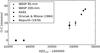 |
Fig. 1 Comparison between observed and computed times of minima for the primary eclipse of AI Phe, using the ephemeris from Hrivnak & Milone (1984). |
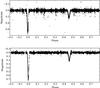 |
Fig. 2 Top: 85-mm WASP-South phase-folded lightcurve for AI Phe. Bottom: phase-folded WASP-South 200-mm data from cameras 225 and 226. |
In all the observations of AI Phe over the last 40 years or so, the secondary eclipse has not been observed in its entirety in one night, so it has not been possible to investigate the timings of the secondary eclipse. This investigation would have given an insight into the possible cause of the apparently quadratic nature of the ephemeris. If the deviations in calculated timings are common to both the primary and secondary minima, it may suggest a third body is involved, or if the deviations have opposite signs then it may suggest apsidal motion is involved.
Figure 2 shows the phase-folded lightcurves for both the 85-mm and 200-mm data using the ephemeris in Eq. (2), having been processed using the method described in Sect. 2.2.
3.2. A Contaminating companion
 |
Fig. 3 2MASS image (combined J, H and Ks bands) of AI Phe showing the close proximity of the contaminating star (Image: Aladin Sky Atlas, Bonnarel et al. 2000). |
An image of AI Phe from the Two Micron All Sky Survey (2MASS, Skrutskie et al. 2006) shows there is another star approximately 11′′ to the east of AI Phe, as shown in Fig. 3. The close proximity of the star means it resides within the aperture used for the WASP photometry of AI Phe and so contributes to the measured flux. As such, it has been necessary to include third light as a parameter that is fitted during the lightcurve analysis.
Although seen in the 2MASS images, this survey does not present any photometric measurements for this companion star. Near-infrared photometry for this star was taken from the Deep Near-Infrared Survey (DENIS, Epchtein et al. 1997), with I = 13.50 ± 0.02 mag, J = 12.95 ± 0.07 mag and K = 12.60 ± 0.14 mag. The I − J, J − K, and I − K colours for the companion were compared to the Dartmouth stellar evolution models (Dotter et al. 2008), and by assuming a main-sequence star with [ Fe/H ] = 0.0 and an age 2 Gyr, its mass was estimated as 0.91 ± 0.06 M⊙. This was used to obtain expected absolute magnitudes from the Dartmouth model, which were in turn used to calculate the distance modulus in each band, resulting in an estimated distance of 590 ± 9pc to the companion. Comparing this value with the distance to AI Phe of 162 ± 6 pc (Andersen et al. 1988), we conclude that the visual companion is not physically associated with the system.
3.3. Model
This work uses the ebop lightcurve analysis code (Nelson & Davis 1972; Popper & Etzel 1981). The subroutine light from this code, which calculates the lightcurves at specified orbital phases for a given set of model parameters, was converted to double-precision floating point arithmetic and modifications were made to enable it to be called directly from the programming language, Python. The ebop lightcurve is then combined with the least-squares Levenberg-Marquardt, Python module, MPFIT (Markwardt 2009) to find the best-fit parameters, i.e. the parameters that minimise the χ2 value between the model and data.
The following seven parameters were allowed to vary during the fitting process: surface brightness ratio at the centre of the stellar discs, J; sum of the radii, rsum = r1 + r2; ratio of the radii, k = r2/r1; inclination, i; ecosω, esinω; third-light, l3. In addition to these fitted parameters, the fractional radii, r1 and r2 are automatically calculated from rsum and k, while the eccentricity e and longitude of periastron ω are calculated from ecosω and esinω.
The mass ratio, q = M2/M1, was fixed at 1.0418, taken from Hełminiak et al. (2009). This is slightly larger than the value 1.034 quoted by Andersen et al. (1988), but modifying the mass ratio by such a small amount had no effect on the best-fit parameters. The gravity darkening exponents also have little impact on the shape of the lightcurve in the case of AI Phe as the system is well-detached. Using values taken from the table by Claret & Bloemen (2011), the gravity darkening exponent for the primary, yp, and secondary, ys, were fixed at 0.26 and 0.50 respectively. The same values were used for both the 85-mm and 200-mm data.
The linear limb-darkening coefficients were also held fixed. Attempts were made to include these as free parameters, but we found that they are not usefully constrained by the data. Instead, the limb darkening coefficients were estimated by interpolation in the table of Claret & Bloemen (2011) by using values for effective temperature, surface gravity and metallicity for the two components from Andersen et al. (1988). For the 85-mm data we adopted the primary limb darkening coefficient, up = 0.54 ± 0.03 and us = 0.67 ± 0.03 for the secondary. For the 200-mm data we used up = 0.52 ± 0.05 and us = 0.67 ± 0.05 using the Kepler pass-band to approximate the response of the WASP broad-band filter. To account for the uncertainties in the limb darkening coefficients, each coefficient was varied by its error and a new model fitted. For each parameter, the average absolute difference between these models and the best fit model has been added in quadrature to the uncertainties from the best-fit parameters. Table 3 details the typical contribution to the uncertainty of each parameter, for both the 200-mm and 85-mm data. These were calculated from the mean contributions for each best-fit detailed in Sects. 3.6 and 3.7.
Typical uncertainty contribution to each parameter from uncertainty limb darkening coefficients.
3.4. Parameter-Space Exploration with emcee
One of the greatest risks when using a least squares minimisation method is that the solution that is found is a local minimum, rather than the overall global minimum of the problem. If local minima are present it is important that these are considered when the uncertainties for the final parameters are calculated. Markov chain Monte Carlo (MCMC), in the form of the Python module, emcee, (Goodman & Weare 2010) was used to check for these local minima, within the parameter-space of the same seven parameters used in the model fitting (J, rsum, k, i, ecosω, esinω and l3). emcee uses the affine-invariant ensemble sampling (stretch-move) algorithm developed by Goodman & Weare (2010), where a group of walkers explore the parameter space. This group of walkers can be split allowing the process to be run in parallel and the affine-invariant transformations mean the algorithm can cope with skewed probability distributions. The positions of the walkers within a particular sub-group are updated using the positions of walkers in the other subgroups.
The probability that a model produced by the parameters from the walkers, corresponds to
the best-fit model is evaluated using the log likelihood function ![Mathematical equation: \begin{equation} \ln \mathcal{L}({\vec{y}}; {\bf \Theta}) = -\frac{1}{2} \sum^N_{n=1} \left[ \left(\frac{m_{n}-y_{n}({\bf \Theta})}{m_{{\rm {err,}}n}}\right)^2 - \ln \left( \frac{2\pi}{m_{{\rm{ err,}}n}^2}\right) \right] \label{eq:loglike} \end{equation}](/articles/aa/full_html/2016/07/aa28581-16/aa28581-16-eq114.png) (3)where y is a vector
of length N
containing the magnitudes generated for a model, Θ is a vector containing the varying
parameters (J, rsum, k, i, ecosω,
esinω and l3),
m is the
observed magnitude and merr is the standard error on the
magnitude. Priors were applied, but these are only used to prevent the parameter exploring
areas that are unphysical, eg. rsum or J being less than zero.
(3)where y is a vector
of length N
containing the magnitudes generated for a model, Θ is a vector containing the varying
parameters (J, rsum, k, i, ecosω,
esinω and l3),
m is the
observed magnitude and merr is the standard error on the
magnitude. Priors were applied, but these are only used to prevent the parameter exploring
areas that are unphysical, eg. rsum or J being less than zero.
The process ran using 150 walkers for 2500 steps, of which the first 200 were discarded to allow for an adequate burn-in stage. For each of the walkers, a starting point for each parameter was chosen by choosing a number at random from a normal distribution (with a mean of zero and variance of 0.01) and adding it to the best-fit parameter. While this method would initially create a ball of walkers close to the solution found by the model, the burn-in stage allows the walker to spread out from this ball. Each parameter was subsequently checked, by plotting the walkers’ positions against step number, to ensure the burn-in stage was completed within these first 200 steps. To ensure the was no bias from the walkers’ starting positions, a test was run that allowed the walkers to start further from the model solution, up to three times the parameters’ uncertainties as determined from the covariance matrix of the best-fitting model. The burn-in stage for this test was much longer, but also failed to reveal any other local minima, so we concluded the original starting points were adequate.
Figure 4 shows example distributions for the 85-mm data. The contours plotted over the top of the distributions indicate the density of points with the darker regions showing higher densities towards the centre of each plot. The grey lines across each of the distributions show where the best-fit values lie. Generally the resulting distributions are symmetric, as shown by the histograms for each parameter. However, there are correlations between some of the parameters, as seen by the tilted ellipsoid shaped regions. Many of these correlations link the third-light parameter to the other parameters, more specifically there are strong correlations between l3 and J, k and i. The correlation with k highlights the importance for the inclusion of the third-light parameter in the model, because without it, the resulting relative radii would be subject to a systematic error.
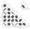 |
Fig. 4 Density distribution of parameter space explored using MCMC. The best-fit parameters as determined by the model are marked by the grey crosses on the density distributions, and the grey line on the histograms. The contours on each of the distributions indicate the density of the points, with the darker, denser regions towards the centre of each plot. The distribution for r1 and r2 has been calculated from k and rsum. Data shown is for the 85-mm original data, without priors. |
3.5. Prayer-bead error analysis
It is inappropriate to use the covariance matrix from the least-squares fit to estimate the standard errors on the model parameters. This is because the assumption of uncorrelated noise with a Gaussian distribution is not satisfied for WASP photometry. It is not clear that the distribution of points from the MCMC chain gives an accurate impression of the posterior probability distribution of the parameters, for the same reason. Therefore, it is not appropriate to use the likelihood calculated using Eq. (3) either. As such, the standard errors on the best-fit parameters have been calculated using a prayer-bead (residual permutation) as described by Southworth (2008) and based on an algorithm developed by Jenkins et al. (2002). The residuals between the data and the best-fit model are shifted by a number of steps to create a synthetic data set. A new model is then fitted to this synthetic data, and the process is repeated across the entirety of the original data set. The uncertainties are the standard deviation of the fitted parameters from all the synthetic data models. Ideally, the number of shifts would be N − 1, where N is the number of observations used in generating the best-fit model. However, due to the large number of points involved in the WASP lightcurves, the number of shifts used was restricted to 500 spread evenly across the data. To ensure the best-fit solution was not affected by the choice of initial parameters, the initial parameters were taken at random from positions within the MCMC analysis.
3.6. Detrending Investigations
Best-fit parameters for AI Phe from 85-mm and 200-mm data, with and without the detrending applied.
As mentioned in Sect. 2.1, WASP photometry is
processed using the detrending algorithm described in Collier Cameron et al. (2006). The algorithm is used to remove four trends of
systematic errors which are common to all stars in a particular field and is given by the
equation 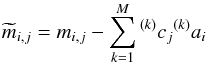 (4)where mi,j and
 are the observed and corrected magnitude,
respectively, for star j at time i. M is the total number of trends, ai are basis functions
detailing the patterns of systematic errors and cj describes to what
extent each basis function affects a particular star. The algorithm is applied separately
to each unique combination of camera and season, and aids the process locating planetary
transits by flattening lightcurves over the time scale of a typical transit length (2.5
h). The work in this paper aims to determine the radii of AI Phe to the highest accuracy
possible using the WASP photometry, and so the effects of the detrending process on the
resulting parameters have been investigated.
are the observed and corrected magnitude,
respectively, for star j at time i. M is the total number of trends, ai are basis functions
detailing the patterns of systematic errors and cj describes to what
extent each basis function affects a particular star. The algorithm is applied separately
to each unique combination of camera and season, and aids the process locating planetary
transits by flattening lightcurves over the time scale of a typical transit length (2.5
h). The work in this paper aims to determine the radii of AI Phe to the highest accuracy
possible using the WASP photometry, and so the effects of the detrending process on the
resulting parameters have been investigated.
Reversing the detrending entirely would re-introduce all the systematic errors the
algorithm was designed to remove, making comparisons between the resulting parameters more
difficult. Instead, effective detrending coefficients, c′, have been calculated.
These coefficients take into consideration the variability of an eclipsing binary, by
including a lightcurve model, L, when they are calculated. For AI Phe, the
situation can be described using 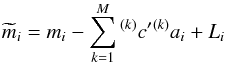 (5)where mi and
 are the observed and corrected magnitude
(respectively) for AI Phe, and
are the observed and corrected magnitude
(respectively) for AI Phe, and  are the same detrending basis functions as
before. The effective detrending coefficients for each of the basis functions were
calculated using singular value decomposition (SVD). Effects from the altered detrending
coefficients were removed from the observed data, then using ebop and MPFIT,
best-fit parameters were obtained. A best-fit model generated using the method in Sect.
3.3, was used for L initially. However, to
ensure the choice of initial model did not bias the results, the values of c′ were calculated for
multiple models. This was done as an iterative process, which continued until all
parameters change by less than 0.005% with each new model. Once the final set of best-fit
parameters was determined, MCMC and prayer-bead analysis were used to calculate their
associated uncertainties.
are the same detrending basis functions as
before. The effective detrending coefficients for each of the basis functions were
calculated using singular value decomposition (SVD). Effects from the altered detrending
coefficients were removed from the observed data, then using ebop and MPFIT,
best-fit parameters were obtained. A best-fit model generated using the method in Sect.
3.3, was used for L initially. However, to
ensure the choice of initial model did not bias the results, the values of c′ were calculated for
multiple models. This was done as an iterative process, which continued until all
parameters change by less than 0.005% with each new model. Once the final set of best-fit
parameters was determined, MCMC and prayer-bead analysis were used to calculate their
associated uncertainties.
Table 4 contains the best-fit parameters for both the 85-mm and 200-mm, with the difference between the original data and detrended data included for comparison. With the exceptions of J and l3 for the 200-mm data and ecosω for the 85-mm, all the best-fit parameters for the detrended data lie within the uncertainties of the parameters from the original data. Therefore, in general, the detrending algorithm applied during the WASP pipeline does not affect the overall best-fit parameters. The large difference present for J and l3 for the 200-mm data is due to the quality of the data present in the primary eclipse. The eclipse is covered by the two cameras on one night, and there is an offset between the data from the two cameras. This maybe be due to the differences in the transmission profile of the filters used in different cameras. In the detrended case, the model shifts enough to favour the data from camera 226, which forms a deeper eclipse. This results in the larger value of J and, because the surface brightness is strongly correlated with l3, there is the corresponding decrease in l3. Figures 5 and 6 show the best-fit model plotted against the detrended data for the 85-mm and 200-mm data, respectively. The fit residuals are also shown in these figures.
As the sets of parameters from the original and detrended data are generally consistent, but the uncertainties associated with the detrended parameters are smaller, it is the detrended parameters that will be used from now on.
3.7. Constraining ecosω and esinω
Best-fit parameters for AI Phe from detrended 85-mm and 200-mm data, with the priors, ecosω = −0.064 ± 0.004 and esinω = 0.176 ± 0.003.
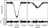 |
Fig. 5 Upper panels: detrended best-fit model for AI Phe (grey line) plotted over the 85-mm WASP-South photometry for the primary (left) and secondary (right) eclipses. Lower panels: residuals between the plotted model and the data, with the grey line marking zero. |
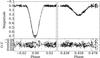 |
Fig. 6 Upper panels: detrended best-fit model for AI Phe (grey line) plotted over the 200-mm WASP-South photometry for the primary (left) and secondary (right) eclipses. Lower panels: residuals between the plotted model and the data, with the grey line marking zero. |
In Table 4, between the 85-mm and 200-mm parameters, there are differences of 2.7σ and 4σ for e and ω, respectively. The values also differ from the values quoted by Hełminiak et al. (2009) and Andersen et al. (1988), e: 0.187(4) and 0.188(2) respectively; ω: 110.1(9)° and 109.9(6)°, respectively. To investigate further, ecosω and esinω were fixed at −0.06424 and 0.17561, respectively. These values were calculated from the spectroscopic e and ω of Hełminiak et al. (2009) and were chosen over Andersen et al. (1988), as the Hełminiak et al. values were obtained more recently. If the orbit has been varying (see Sect. 3.1), the most recent values should be nearest to those applicable to the time span covered by the WASP data.
However, fixing ecosω and esinω produced models that were poor fits to the data. This was the case for both the 85-mm and the 200-mm data, but was more significant in for the 85-mm. For the 85-mm data, there was a phase offset of 0.001 between the observed data and resulting model of the secondary eclipse.
As an alternative to fixing ecosω and esinω, the values calculated from Hełminiak et al. (2009) with their standard errors were used as Gaussian priors during the model fitting. Table 5 contains the best-fit parameters for the detrended 85-mm and 200-mm data, with inclusion of the priors. Again, the uncertainties have been calculated through MCMC and prayer-bead analysis, and the error contribution from the uncertainties in the limb darkening value has also been included. For the 85-mm data, the inclusion of the priors has altered the best-fit parameters by less than their uncertainties. e and ω have been altered more significantly for the 200-mm data, bringing their values closer to those of the 85-mm data. However, the values for both are still inconsistent with each other.
The exact cause of the differing e and ω values remains unclear. Previous observations of AI Phe have yielded a range of values for e and ω. For example, Hrivnak & Milone (1984) found e = 0.1726 ± 0.0006 and ω = (111.8 ± 0.1)° giving ecosω = −0.06410 ± 0.00007 and esinω = 0.1603 ± 0.0007, while the same UBVRI lightcurve analysed by Andersen et al. (1988) yielded mean values of ecosω = − 0.064 and esinω = 0.183. No clear trend is present when all available value of ω were plotted against time, as might be expected if these differences are due to apsidal motion. The parameter esinω is very sensitive to the shape of the secondary eclipse. Without observing the base of the secondary eclipse in one night, defining the exact shape of the eclipse and therefore determining the value of esinω can be difficult. Values of e and ω determined from spectroscopic orbits will not suffer these problems and should therefore be more accurate. It seems there is still work to be done in order to completely understand the behaviour of AI Phe’s orbit.
Despite the inconsistency of e and ω, the addition of the priors has had very little impact on r1 and r2. They have remained consistent with each other, with a small reduction in the uncertainties of the 200-mm data. The radii are determined by the contact points, which are well defined by the primary eclipse, and the ratio of the eclipses k, but only as k0.25. Therefore, r1 and r2 are robustly measured despite problems with the secondary eclipse and small changes in the 200-mm eclipse depth. A number of the other parameters have also shown small reductions in their uncertainties, and therefore the best-fit parameters obtained with the priors have been used in further analysis.
3.8. Overall best-fit parameters
Table 6 summarises the results from the lightcurve analysis, and includes the sets of best-fit parameters from the detrended 85-mm and 200-mm data, obtained with priors. For comparison, the results of Andersen et al. (1988) are also included in the table. As the two WASP data sets and the results of Andersen et al. (1988) are all independent, they have been combined to produce an overall weighted mean. Uncertainties from each of the parameters were used to calculate internal and external standard errors on these mean values (i.e. based on the error bars and scatter, respectively), with the larger of the two being quoted alongside the weighted means. For r1 and r2 the results were internally consistent. The mean surface brightness ratio and third-light are not included because the different filters were used to obtain the 200-mm and 85-mm data.
AI Phe lightcurve parameters summary from this study, and comparative results from Andersen et al. (1988).
4. Absolute parameters
As mentioned in Sec. 1, Hełminiak et al. (2009) obtained high precision radial velocity measurements for AI Phe and combined these with ASAS photometric measurements to derive the masses and radii of the two components of AI Phe. The values they used for the semi-amplitude velocities K1 and K2 are 51.36(3) km s-1 and 49.11(2) km s-1 respectively.
Absolute parameters for AI Phe parameters calculated using lightcurve parameters from this work and spectroscopic values from Hełminiak et al. (2009), with comparisons to previous work.
The WASP photometry provides more complete lightcurves for AI Phe than the ASAS data, and therefore it has been possible to obtain the lightcurve parameters to a higher precision. Using the weighted means for r1, r2, e and i from the Table 6 and the semi-amplitude velocities from Hełminiak et al. (2009), masses and radii of the stars within AI Phe have been calculated and are shown in Table 7. jktabsdim1 was used for this, as were the constants as suggested by Torres et al. (2010). Table 7 also contains results from Andersen et al. (1988) and Hełminiak et al. (2009) for comparison. Note that the uncertainties of M1,2sin3i and the masses quoted by Hełminiak et al. have been recalculated using jktabsdim. Their uncertainties have been underestimated somewhat as their quoted uncertainties could not be reproduced with jktabsdim, despite using all values quoted in their paper. With the uncertainties in K1 and K2 being so small, the uncertainty in the eccentricity has become the largest source of error in the masses. Overall, the values obtained in this work for M1,2sin3i do have larger uncertainties than those of Hełminiak et al., which is due to the greater uncertainty in the eccentricity, but with the improved accuracy of the inclination, the uncertainties in the masses has been reduced to 0.31% for both M1 and M2. While M1 is consistent with the value found by Andersen et al. (1988), there is almost a 3σ difference in M2. This stems from different M2sin3i, and so it is also seen in the values from Hełminiak et al.
There has also been a significant reduction in the uncertainties associated with the radii. R1 is known to a precision of 0.76% while R2 is known to a precision of 0.48%, a reduction from 1.3% and 1.6% respectively (Andersen et al. 1988). Although not a concern for the radii presented here, below 0.1% precision, uncertainties in the constant used for the solar radius, and the definition of a star’s radius needs to be considered (Torres et al. 2010).
The biggest contribution to the uncertainties of the masses is now the eccentricity. Further reduction in the uncertainties of the masses would require the orbit of AI Phe to be better understood, and an understanding of the variability shown in e and ω.
5. Implication for models
The increase in precision associated with the masses and radii of AI Phe will provide tighter constraints on the models that can provide an estimate of the age of the system. As such, a MCMC method has been used to estimate the age of AI Phe for a number of grids of models, with varying mixing length, αml and helium abundance, Y. The grids of models have been produced with the garstec stellar evolution code (Weiss & Schlattl 2008) and methods used to calculate the grids are described by Maxted et al. (2015b) and Serenelli et al. (2013). The MCMC method is very similar to the method described by Maxted et al. (2015b), however there are a number of differences, which are described in more detail in Sects. 5.1 and 5.2. Most notably, the code will attempt to fit the two stars of AI Phe to the same isochrone instead of fitting each star individually. The priors have also been modified slightly in order to accommodate the new observed values for both stars.
garstec uses the Kippenhahn & Weigert (1990) mixing length theory for convection, where αml = 1.78 produces the observed properties of the Sun assuming the composition given by Grevesse & Sauval (1998), an initial solar helium abundance Y⊙ = 0.26626, and initial solar metallicity Z⊙ = 0.01826. The initial solar composition corresponds to an initial iron abundance of [Fe/H]i = + 0.06, due the effects of microscopic diffusion. OPAL radiative opacities of Iglesias & Rogers (1996) are used and are complemented by molecular opacities from Ferguson et al. (2005) at low temperatures.
Convective mixing is treated as a diffusive process, where the diffusion coefficient at
each point is given by  . αmlHP is the
local mixing length, and vc is the convective velocity determined
from mixing length theory. Overshooting is included by extending the mixing region beyond
the formal Schwarzschild boundary with an exponentially decaying diffusion coefficient,
given as D =
D0exp( − 2z/
(fhp)). D0 is the
diffusion coefficient inside the convective border, f = 0.020 is a free parameter
defining the scale of overshooting and
. αmlHP is the
local mixing length, and vc is the convective velocity determined
from mixing length theory. Overshooting is included by extending the mixing region beyond
the formal Schwarzschild boundary with an exponentially decaying diffusion coefficient,
given as D =
D0exp( − 2z/
(fhp)). D0 is the
diffusion coefficient inside the convective border, f = 0.020 is a free parameter
defining the scale of overshooting and
![Mathematical equation: \begin{equation} h_{\rm p} = H_{\rm P} \times {\rm min} \left[1, \left( \frac{\Delta R_{\rm CZ}}{H_{\rm P}} \right)^{2} \right]\cdot \end{equation}](/articles/aa/full_html/2016/07/aa28581-16/aa28581-16-eq334.png) (6)ΔRCZ is the thickness of the convective
core, and HP is the pressure scale height. The
definition of hp ensures that for small convective
regions, (particularly small convective cores where ΔRCZ<HP)
the overshooting region is geometrically limited to a fraction of the size of the convective
region (Magic et al. 2010). If RCZ>HP the
geometric limit does not play a role and the overshooting region amounts to ~0.25HP, for
convective cores in the main sequence. For stars in the range 1.2−1.3 M⊙, when a
convective core develops towards the end of the main sequence, the geometric cut effectively
limits the size of the overshooting region to ~0.05HP.
(6)ΔRCZ is the thickness of the convective
core, and HP is the pressure scale height. The
definition of hp ensures that for small convective
regions, (particularly small convective cores where ΔRCZ<HP)
the overshooting region is geometrically limited to a fraction of the size of the convective
region (Magic et al. 2010). If RCZ>HP the
geometric limit does not play a role and the overshooting region amounts to ~0.25HP, for
convective cores in the main sequence. For stars in the range 1.2−1.3 M⊙, when a
convective core develops towards the end of the main sequence, the geometric cut effectively
limits the size of the overshooting region to ~0.05HP.
Atomic diffusion of all atomic species is included by solving the multi-component flow equations of Burgers (1969), according to the method of Thoul et al. (1994). Extra macroscopic mixing below the convective envelope is also included. It follows the parametrisation given in VandenBerg et al. (2012) and depends on the extension of the convective envelope. Radiative accelerations and stellar winds are not included in model calculations for main-sequence stars. These effects become more relevant as stellar mass is increased and limit the efficiency of atomic diffusion which, if acting alone, would yield metal abundances in the stellar surface much lower than observed. For this reason, the efficiency of atomic diffusion is smoothly decreased in models from 1.25−1.35 M⊙ and completely switched off for higher masses.
The model grids used cover six different mixing lengths, (1.22, 1.36, 1.50, 1.78, 2.04 and
2.32) with the helium abundance YAI fixed. An additional ten model grids
have helium abundances that change by ΔY from an initial value in increments of 0.01,
whilst the mixing length is fixed. ΔY covers a range from −0.05 to 0.05. The initial value, Y0 = 0.261 ± 0.007
was calculated using 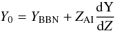 (7)where YBBN = 0.2485 is
the primordial helium abundance at the time of the big-bang nucleosynthesis (Steigman 2010), and ZAI = 0.012 ±
0.007 is the initial metal content of AI Phe. Diffusion has been
considered with the chosen ZAI, however, the effect is almost
negligible, making ZAI nearly identical to the surface
Z (Andersen et al. 1988). dY/ dZ is an
assumed helium-to-metal enrichment calculated as dY/ dZ = (Y⊙ −
YBBN) /Z⊙ =
0.984 using Z⊙ =
0.01826 and Y⊙ = 0.26626 (Maxted et al. 2015b). The value of dY/ dZ is
very uncertain. Here, we have used a solar calibrated value, however dY/ dZ can
change depending on where in the Galaxy you look and values in the literature can range from
0.5 to 5 (Lebreton et al. 2014; Gennaro et al. 2010). Lebreton et al.
(2014) showed that increasing dY/ dZ from 2 to 5, decreases the
turn off age of the star. The mass range 0.6
M⊙ to 2.0 M⊙ is covered
by the model grids, in steps of 0.02
M⊙, while the initial metallicity,
[Fe/H]i covers
−0.75 to −0.05 in steps of 0.1 dex and −0.05 to + 0.55 in steps of 0.05 dex.
(7)where YBBN = 0.2485 is
the primordial helium abundance at the time of the big-bang nucleosynthesis (Steigman 2010), and ZAI = 0.012 ±
0.007 is the initial metal content of AI Phe. Diffusion has been
considered with the chosen ZAI, however, the effect is almost
negligible, making ZAI nearly identical to the surface
Z (Andersen et al. 1988). dY/ dZ is an
assumed helium-to-metal enrichment calculated as dY/ dZ = (Y⊙ −
YBBN) /Z⊙ =
0.984 using Z⊙ =
0.01826 and Y⊙ = 0.26626 (Maxted et al. 2015b). The value of dY/ dZ is
very uncertain. Here, we have used a solar calibrated value, however dY/ dZ can
change depending on where in the Galaxy you look and values in the literature can range from
0.5 to 5 (Lebreton et al. 2014; Gennaro et al. 2010). Lebreton et al.
(2014) showed that increasing dY/ dZ from 2 to 5, decreases the
turn off age of the star. The mass range 0.6
M⊙ to 2.0 M⊙ is covered
by the model grids, in steps of 0.02
M⊙, while the initial metallicity,
[Fe/H]i covers
−0.75 to −0.05 in steps of 0.1 dex and −0.05 to + 0.55 in steps of 0.05 dex.
5.1. Input data
For the MCMC analysis, a vector of parameters d = (T1, ρ1, ρ2, Tratio, Msum, q, [ Fe/H ] s) can be used to define the observed quantities for AI Phe. These parameters have been chosen because each quantity is determined by an independent feature of the data used in the analysis, with little or no dependence on the other parameters. Tratio is the ratio of the effective temperatures given by T2/T1, T1 and T2 are the effective temperatures of the two stars, ρ1 and ρ2 are the average stellar densities of the two stars, Msum is the sum of their masses, q is the mass ratio given by M2/M1 and [Fe/H]s is the observed surface metal abundance.
The mass ratio and sum of the masses were chosen over directly using the individual
masses M1 and M2, as the
individual masses have stronger correlations. The densities of the two stars
(ρ1 = 0.1935 ±
0.0044 ρ⊙ and ρ2 = 0.0505 ± 0.0007
ρ⊙) were calculated using 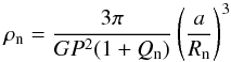 (8)where R is the radius for star
n = 1,2,
a is the
semi-major axis of the orbit, P is the orbital period, G is Newton’s gravitational
constant (Maxted et al. 2015b). Qn is a function
of the mass ratio, where Q1 = q and
Q2 = 1
/q. Equation (8) allows the density to be calculated directly from values of
r1 and r2 derived from
the lightcurve analysis using Kepler’s law, and independently from the mass estimates from
the spectroscopic orbit. T1 was taken to be 6310 ± 150 K (Vandenberg & Hrivnak 1985).
(8)where R is the radius for star
n = 1,2,
a is the
semi-major axis of the orbit, P is the orbital period, G is Newton’s gravitational
constant (Maxted et al. 2015b). Qn is a function
of the mass ratio, where Q1 = q and
Q2 = 1
/q. Equation (8) allows the density to be calculated directly from values of
r1 and r2 derived from
the lightcurve analysis using Kepler’s law, and independently from the mass estimates from
the spectroscopic orbit. T1 was taken to be 6310 ± 150 K (Vandenberg & Hrivnak 1985).
The ratio of the stars’ effective temperatures can be determined directly from the surface brightness ratio derived from the lightcurve analysis. The surface brightness ratio is related to the ratio of the eclipse depths in a totally-eclipsing binary, with very little dependence on the other parameters of the lightcurve. An approximate value of Teff is needed for one of the stars in the binary, but this value has only a small effect on the derived Tratio. Our method uses Kurucz (1993) model atmospheres and the profiles for numerous passbands, (Bessell 1990; Crawford & Barnes 1970; Doi et al. 2010) and is similar to the method described by Maxted et al. (2015a). For each of the bands, Johnson BVRI, Strömgen y and SDSS r′, a relationship was established between effective temperature and surface brightness for log g = 4.0 and log g = 3.6. Interpolation between the values from the models for log g = 4.0 and log g = 3.5 was used in the case of log g = 3.6 as no model was available. Taking T1 = 6310 ± 150 K we used these relationships to find a value for T2 that gave the measured average surface brightness ratio for each band. The average surface brightness ratios were calculated from the central surface brightness ratios for the BVRI and y passbands from Andersen et al. (1988) and the 85-mm central surface brightness ratio was used for SDSS r′ passband. Andersen et al. (1988) did not define their surface brightness ratios as average or central values. We have assumed the values are central surface brightness ratios because their lightcurve model uses the same methods as ebop and should therefore produce the same ratios as ebop. Following the example of Andersen et al. (1988), limb darkening coefficients for the BVRI were taken from Hrivnak & Milone (1984) and limb darkening coefficients for y from Wade & Rucinski (1985). The values of Tratio derived using this method for the different passbands were found to be consistent with each other. The weighted mean and standard error are Tratio = 0.83 ± 0.01, where the standard error estimate accounts for the uncertainties on both J and T1. There are surface brightness ratios available for the Johnson U and Strömgen uvb passbands in the Andersen et al. (1988) paper, however this method is less reliable in the bluer passbands as line-blanketing is more prevalent. These bands were therefore excluded from the determination of Tratio. Another consideration is the metallicity used by the models. The Kurucz (1993) model atmospheres consider solar metallicity, instead of the measured value of AI Phe (−0.14 ± 0.1, Andersen et al. 1988). However, Maxted et al. (2015a) found that changing the metallicity by ± 0.1 dex changes the resulting T2 by less than 10 K, or ≈ 0.002 in Tratio. As such, the resulting error is within the uncertainties of Tratio.
5.2. Bayesian age estimates
The model parameters used to predict the observed data can be represented as
![Mathematical equation: \hbox{$\vec{m} = \left(\tau_{\rm sys}, M_{1}, M_{2}, \mathrm{[Fe/H]}_{\mathrm{i}}\right)$}](/articles/aa/full_html/2016/07/aa28581-16/aa28581-16-eq397.png) , where τsys,
M1, M2 and
[ Fe/H ] i are
the age, mass of star 1, mass of star 2, and initial metal abundance of the system,
respectively. Due to diffusion and mixing processes occurring in the star during its
evolution, the initial metal abundance, [ Fe/H
] i differs from the observed surface metal abundance,
[ Fe/H ] s.
, where τsys,
M1, M2 and
[ Fe/H ] i are
the age, mass of star 1, mass of star 2, and initial metal abundance of the system,
respectively. Due to diffusion and mixing processes occurring in the star during its
evolution, the initial metal abundance, [ Fe/H
] i differs from the observed surface metal abundance,
[ Fe/H ] s.
The probability distribution function p(m | d)
∝ ℒ(d |
m)p(m)
was determined using a MCMC method. ℒ(d | m) =
exp(−χ2/ 2) is used to estimate the
likelihood of observing the data d for a given model m, where
![Mathematical equation: \begin{eqnarray} \chi^2 &= & \left[\sum_{n=1,2}\frac{\left(\rho_{n} - \rho_{n,\mathrm{obs}}\right)^2}{\sigma_{\rho_{n}}^2} \right] +\frac{\left(T_{\mathrm{1}} -T_{\mathrm{1,obs}}\right)^2}{\sigma_{T_{1}}^2} + \frac{\left(T_{\rm ratio} - T_{\rm ratio, \mathrm{obs}}\right)^2}{\sigma_{T_{\rm ratio}}^2} \\ && + \frac{\left(M_{\rm sum} - M_{\rm sum, \mathrm{obs}}\right)^2}{\sigma_{M_{\rm sum}}^2} + \frac{\left(q - q_{\mathrm{obs}}\right)^2}{\sigma_{q}^2} + \frac{\left(\mathrm{[Fe/H]}_{\mathrm{s}} - \mathrm{[Fe/H]}_{\mathrm{s,obs}}\right)^2}{\sigma_{\mathrm{[Fe/H]_{\mathrm{s}}}}^2} \nonumber\cdot \end{eqnarray}](/articles/aa/full_html/2016/07/aa28581-16/aa28581-16-eq405.png) (9)Observed quantities are denoted with “obs”
subscript and their standard errors are given by the appropriately marked σ. The probability
distribution function p(m) =
p(τsys)p(M1)p(M2)p(
[ Fe/H ] i) is the product of the individual priors on each
of the model parameters. The assumed prior on [
Fe/H ] i normally has little effect because this parameter
is well constrained by the observed value of [
Fe/H ] s so a ‘flat’ prior on [ Fe/H ] i is used, i.e., a
uniform distribution over the model grid range. Although there is a prior on the age to
keep it within the limits of 0 – 17.5 Gyr, the age does not venture close to these limits
as the other priors provide much tighter constraints on the age of the system. The code
also offers the option to set a prior on the surface [ Fe/H ] for cases where there is no
observed value of surface metallicity. As the [
Fe/H ] s is tightly constrained from observation, a flat
prior of −0.75 < [ Fe/H ] <
0.55 was used.
(9)Observed quantities are denoted with “obs”
subscript and their standard errors are given by the appropriately marked σ. The probability
distribution function p(m) =
p(τsys)p(M1)p(M2)p(
[ Fe/H ] i) is the product of the individual priors on each
of the model parameters. The assumed prior on [
Fe/H ] i normally has little effect because this parameter
is well constrained by the observed value of [
Fe/H ] s so a ‘flat’ prior on [ Fe/H ] i is used, i.e., a
uniform distribution over the model grid range. Although there is a prior on the age to
keep it within the limits of 0 – 17.5 Gyr, the age does not venture close to these limits
as the other priors provide much tighter constraints on the age of the system. The code
also offers the option to set a prior on the surface [ Fe/H ] for cases where there is no
observed value of surface metallicity. As the [
Fe/H ] s is tightly constrained from observation, a flat
prior of −0.75 < [ Fe/H ] <
0.55 was used.
The Markov chain setup uses the same approach described by Maxted et al. (2015b), in that a Markov chain of points mi is created with the probability distribution p(m | d) using a jump probability distribution f(Δm). The generation of each trial point m′ = mi + Δm is dictated by the probability distribution, with the point being rejected if any of the model parameters are outside of the ranges set by the priors. If ℒ(m′ | d) > ℒ(mi | d), the point is always included, and when ℒ(m′ | d) < ℒ(mi | d) the point is included with probability ℒ(m′ | d)/ℒ(mi | d) (Metropolis-Hastings algorithm). mi + 1 = m′ if the trial point is accepted, or mi + 1 = mi otherwise (Metropolis et al. 1953; Hastings 1970).
In comparison to Maxted et al. (2015b), a different approach is used to find a starting point. Their approach takes the point with the lowest χ2 when a sample of points are randomly generated across the model grid. In our case, because the parameter-space is so well constrained, the starting point needed to be guided towards the parameter-space. The measured masses and metallicity are fixed and used to generate an evolutionary track for each star in the system. From there, each point along the tracks is searched to find the point with the lowest χ2, using 2000 steps in age. This is done separately for the main-sequence and post main-sequence stages, with the best-fit point from this process is used as an initial starting point.
For each parameter a step size is found such that  , where
 denotes a set of model parameters that
differs from m0 only in the value of one
parameter, j.
From there, a burn-in stage of 10 000 steps is used to improve the initial set of
parameters and to determine correlations between parameters by calculating a covariance
matrix. The eigenvectors and eigenvalues of this matrix are used to determine a set of
uncorrelated, transformed parameters, q =
(q1,q2,q3,q4),
where each of the transformed parameters has unit variance (Tegmark et al. 2004). To estimate the probability distribution
p(m |
d), a second Markov chain of 1 000 000
steps is produced, using a Gaussian distribution for f(Δq) with unit
standard deviation for each of the transformed parameters and the most likely model
parameters as a starting point. With the tight constraints given by the priors, some of
the model grids have a severely restricted parameter-space and so required a large number
of steps to ensure the space was explored. All chains were visually inspected and checked
via a running mean to ensure suitable mixing.
denotes a set of model parameters that
differs from m0 only in the value of one
parameter, j.
From there, a burn-in stage of 10 000 steps is used to improve the initial set of
parameters and to determine correlations between parameters by calculating a covariance
matrix. The eigenvectors and eigenvalues of this matrix are used to determine a set of
uncorrelated, transformed parameters, q =
(q1,q2,q3,q4),
where each of the transformed parameters has unit variance (Tegmark et al. 2004). To estimate the probability distribution
p(m |
d), a second Markov chain of 1 000 000
steps is produced, using a Gaussian distribution for f(Δq) with unit
standard deviation for each of the transformed parameters and the most likely model
parameters as a starting point. With the tight constraints given by the priors, some of
the model grids have a severely restricted parameter-space and so required a large number
of steps to ensure the space was explored. All chains were visually inspected and checked
via a running mean to ensure suitable mixing.
5.3. Model comparisons
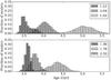 |
Fig. 7 Age distributions of AI Phe obtained for six different values of mixing length, whilst helium abundance is held fixed at zero. Based on Markov chains of 1 000 000 steps. |
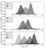 |
Fig. 8 Age distributions of AI Phe obtained for different values of helium abundance whilst fixing the mixing length at 1.78. Based on Markov chains of 1 000 000 steps. |
Age and parameters from the best fitting model from a 1 000 000-step Bayesian age fitting method, for model grids with different mixing lengths and helium abundances.
Using the Bayesian method described in Sects. 5.1 and 5.2 an age distribution has been produced for a number of model grids, with different mixing lengths αml and helium abundance Y. In total, distributions were produced for six mixing lengths (1.22, 1.36, 1.50, 1.78, 2.04 and 2.32) with ΔY held fixed at zero (see Fig. 7) and an additional ten distributions were produced for helium abundances, where ΔY ranged from −0.05 to 0.05 in increments of 0.01, with the mixing length held fixed at 1.78 (Fig. 8). Table 8 contains the parameters from the model with the lowest χ2 for each model grid, alongside the mean τmean and standard deviation στmean of the age distributions produced by the 1 000 000-step chain. In some cases the age distributions produced bimodal distributions which do not fit a Gaussian profile, meaning there is a noticeable difference between the best-fit age τbest and τmean. The first section of the table contains the model grids where αml is varied, and the second section contains model grids where the helium abundance, YAI, is varied by ΔY from the initial value Y0.
The χ2 values in Table 8 show that some of the model grids fit in the parameter-space much
better than others. In terms of the mixing lengths, values of 2.04 and 1.78 are favoured,
with 1.78 producing the lowest χ2. Using the 16th, 50th and 84th
percentiles, a mixing length of 1.78 gives an age of
 Gyr. As the mixing length in the model
grid is increased, the best-fit model tends to increase the mass of the two stars.
Comparing evolutionary tracks for star 2 (the sub-giant) at a fixed age, mass and
metallicity but with increasing mixing length, results in larger densities, as the stars
are more compact (Lebreton et al. 2014). However,
with the tight observational constraints on ρ2, the models attempt to improve the
overall χ2 by increasing M2 and by
decreasing the metallicity. Increasing M2 results in a star with a larger
radius with the same density, but also reduces the age of the sub-giant and therefore the
system. The effect on the age can be seen in the mean and best-fit ages as αml is changed
from 1.50 to 2.32. Decreasing the metallicity allows the system to evolve to the same
evolutionary stage faster.
Gyr. As the mixing length in the model
grid is increased, the best-fit model tends to increase the mass of the two stars.
Comparing evolutionary tracks for star 2 (the sub-giant) at a fixed age, mass and
metallicity but with increasing mixing length, results in larger densities, as the stars
are more compact (Lebreton et al. 2014). However,
with the tight observational constraints on ρ2, the models attempt to improve the
overall χ2 by increasing M2 and by
decreasing the metallicity. Increasing M2 results in a star with a larger
radius with the same density, but also reduces the age of the sub-giant and therefore the
system. The effect on the age can be seen in the mean and best-fit ages as αml is changed
from 1.50 to 2.32. Decreasing the metallicity allows the system to evolve to the same
evolutionary stage faster.
The αml =
1.22 model grid does not follow the mass trend mentioned above, because
the mass distribution is bi-modal, corresponding to two different evolutionary stages. The
most dominant part of the distribution places the secondary very early in the contraction
phase before the ascent to the red-giant branch, with a larger effective temperature. The
less prominent part of the distribution, places the secondary further into the contraction
phase. A similar explanation can be used to explain the sudden change in best-fit age
between αml =
1.36 and αml = 1.50. For the αml = 1.36
model, the secondary component sits firmly in the contraction phase, whereas for
 , the secondary sits at the base
of the red-giant branch.
, the secondary sits at the base
of the red-giant branch.
Increasing the helium abundance used in the model grid has decreased the best-fit age of the system, with the models preferring to use smaller masses and cooler effective temperatures for both stars. The best-fit values for ρ2 show very little variation with helium abundance, changing by less than 1%. Meanwhile, ρ1 shows a much larger variation of 14%. The small uncertainty in M2 tightly constraints the age of the sub-giant, allowing little variation in ρ2. This is not the case with the main-sequence star. In order to find a model for the main-sequence star that fits the age determined by the sub-giant, parameters such as its effective temperature and density need to be varied significantly from their observed value for some values of the helium abundance. This is reflected in their much larger χ2 values.
Looking at the χ2 for the model grid with varying
ΔY in Table
8, the preferred models have a helium abundance
that is closer to the initial value, effectively excluding values where
 and
and
 . The preferred model is where
ΔY = 0.0,
meaning YAI =
0.261. Using Δχ2 = 1 to define a 68.3% confidence
interval on ΔY, based on the projection into the αml-ΔY parameter space (Press et al. 1992), the models for ΔY = −0.01 and
ΔY = 0.02
fall just outside this interval. A Δχ2 = 2.71 defines a 90% confidence
interval and covers the models −0.02 <
ΔY< 0.03. We find
. The preferred model is where
ΔY = 0.0,
meaning YAI =
0.261. Using Δχ2 = 1 to define a 68.3% confidence
interval on ΔY, based on the projection into the αml-ΔY parameter space (Press et al. 1992), the models for ΔY = −0.01 and
ΔY = 0.02
fall just outside this interval. A Δχ2 = 2.71 defines a 90% confidence
interval and covers the models −0.02 <
ΔY< 0.03. We find
 for a fixed mixing length of
1.78, giving an age of
4.39 ± 0.32 Gyr using
τbest from the best-fit model. The
uncertainty is estimated by directly adding στmean from
ΔY = 0
(0.20 Gyr) and a systematic
uncertainty of 0.12 Gyr (from not knowing YAI). For comparison, Torres et al. (2010) found an age of 4.1 Gyr using
experimental Victoria models (VandenBerg et al.
2006) and 5.0 Gyr from Yonsei-Yale models (Demarque et al. 2004), although no uncertainties are given. Spada et al. (2013) found the age of two components of
AI Phe separately using an updated version of the Yale Rotational stellar Evolution Code
(YREC). They find an age of 4.44 ± 0.08
Gyr for the hotter component, and an age of 4.54 ± 0.02 Gyr for the cooler component
meaning our value is consistent with their ages.
for a fixed mixing length of
1.78, giving an age of
4.39 ± 0.32 Gyr using
τbest from the best-fit model. The
uncertainty is estimated by directly adding στmean from
ΔY = 0
(0.20 Gyr) and a systematic
uncertainty of 0.12 Gyr (from not knowing YAI). For comparison, Torres et al. (2010) found an age of 4.1 Gyr using
experimental Victoria models (VandenBerg et al.
2006) and 5.0 Gyr from Yonsei-Yale models (Demarque et al. 2004), although no uncertainties are given. Spada et al. (2013) found the age of two components of
AI Phe separately using an updated version of the Yale Rotational stellar Evolution Code
(YREC). They find an age of 4.44 ± 0.08
Gyr for the hotter component, and an age of 4.54 ± 0.02 Gyr for the cooler component
meaning our value is consistent with their ages.
Comparisons between mixing lengths are quite difficult because of the different approaches to used to calibrate the parameter, and how the mixing length is included in the models. Andersen et al. (1988) used a fixed mixing length of 1.50, which was calibrated by the producing a 1.0 M⊙ star with 1.0 R⊙ and the solar age of 4.7 Gyr. They used interpolation between a solar model and a model with a Z of 0.01 to find the age and helium abundance of AI Phe. Spada et al. (2013) used a similar solar calibration method but found the mixing-length was α = 1.875, and Torres et al. (2010) noted that at the time the Victoria models (VandenBerg et al. 2006) that had not been fully calibrated. Therefore, we note that our best-fit mixing length is the same as the solar value for our set of models. This is consistent with what was found by Andersen et al. (1988).
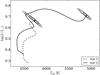 |
Fig. 9 Theoretical tracks for the two components of AI Phe consistent with the best-fit age for the model grid with αml = 1.78 and ΔY = 0.0. 1σ, 2σ and 3σ confidence contours from the Bayesian analysis are shown. |
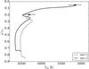 |
Fig. 10 Observed density and effective temperature (Milone et al. 1992) for the two components of AI Phe, for the theoretical tracks consistent with the best-fit age for the model grid with αml = 1.78 and ΔY = 0.0. The uncertainty in the densities are smaller than the markers. |
Figures 9 and 10 show the theoretical tracks for the two components of AI Phe which result in the best-fit age for the model grid with αml = 1.78 and ΔY = 0.0. In Fig. 10, we have plotted the observed densities calculated in this work and the effective temperatures from Milone et al. (1992).
6. Discussion
While the ephemeris in Eq. (2) is suitable for the WASP photometry presented here, it is not suitable for describing the orbit on a long-term basis. It has been shown that the period of AI Phe does not follow a linear ephemeris, with currently available times of primary minimum suggesting it may be more quadratic in nature. The exact cause is not currently known and further work will be needed to determine its nature. Insufficient coverage of the secondary eclipse has prevented us testing how the timings of the secondary eclipse has been affected by these period changes. If the deviations in timings are common to both the primary and secondary minima, it may suggest a third body is involved, or if the deviations are in opposite directions then it may suggest apsidal motion is the cause. Looking for possible trends in the variation in the eccentricity and longitude of periastron with currently available measurements, proved inconclusive. As the eccentricity is now the largest uncertainty in the determination of the masses, understanding the orbit of AI Phe will be essential if the precision of the masses are to be improved further.
The WASP detrending functions have little impact on the determined fractional radii and therefore the radii. Neither did the slight inconsistencies in the determined value of e and ω. In the first case, parameters determined from the 200-mm data have a greater sensitivity to the detrending functions in comparison to the 85-mm data. It is thought to be related to slight variations in the transmission profile of the two filters used, resulting in small differences in the surface brightness and third-light of the 200-mm data. In the second case, the well-defined contact points of the primary eclipse, and the small, fourth-root dependence on k allow the robust measurements of r1 and r2 despite the issues measuring the secondary eclipse.
In the models used for estimating the age of AI Phe, we have assumed that the mixing length and the helium abundance is the same for both of the stars. As the stars are binary components of the same age, they will have formed together from similar material and so using the same initial helium abundance for both stars is valid. As for the mixing length, investigations by Trampedach et al. (2013) found that as stars ascend the giant branch, αml remains constant along the track. However, their calibrations of αml for different Teff and log g using radiation hydrodynamics simulations suggest that the cooler component of AI Phe should have a slightly larger mixing length, due to a difference of 0.4 in log g between the two components and a temperature difference of ≈ 1200 K. This would mean a slightly smaller radius and larger Teff for the star (Spada et al. 2013). The age of the system is largely constrained by the prior on the mass of M2, so a small change in the radius and effective temperature would have little impact on the estimated age.
The models presented here have not explored any potential correlations between the mixing length and helium abundance, due to nature of the model grids. This means a better solution, other than the best-fit solutions in Table 8, could exist elsewhere in the αml-ΔY plane if both αml and ΔY where varied simultaneously. Once we have obtained accurate parameters for four other binary systems, identified using WASP photometry, exploring the αml-ΔY plane is something we intend to do.
Another consideration not explored here is the impact of the convective overshooting on the determined mixing length parameter and helium abundance. The components of AI Phe would provide an important test for convective overshooting as they sit on the mass boundary where stars start to develop convective cores (Lebreton et al. 2014). For a star near the end of the main-sequence star, Valle et al. (2016) found that an uncertainty of ± 1 in the helium-to-metal enrichment ratio, could change the overshooting parameter by ± 0.03, while a variation in αml = 0.24 could change the overshooting parameter from −0.03 to + 0.07. However, they used a different implementation of the overshooting region to the description used in this paper, making it difficult to translate the effects to AI Phe. The effects of convective overshooting is something that should be explored, and tighter constraints on the helium abundance and mixing length should help pin down this parameter.
7. Conclusion
Using WASP photometry, the radii of components in AI Phe were found to be R1 = 1.835 ± 0.014 R⊙ and R2 = 2.912 ± 0.014 R⊙ with the uncertainties in the measurements reduced to 0.76% for R1 and 0.48% for R2. The masses were found to be M1 = 1.1973 ± 0.0037 M⊙ and M2 = 1,.2473 ± 0.0039 M⊙, with their uncertainties reduced to 0.31% for both components. The eccentricity is now the largest source of uncertainty in the masses.
Reducing the uncertainties on the masses and radii of the two stars in AI Phe, has meant
that it has been possible to obtain the age of system, 4.39 ± 0.32 Gyr, with greater precision than
had been achieved by Andersen et al. (1988). From the
different model grids that were tested, a mixing-length of 1.78 and a initial helium
abundance of  gave the best-fit with the priors set by
observations.
gave the best-fit with the priors set by
observations.
Overall, with the new masses and radii obtained with the WASP photometry and spectroscopic orbit data of Hełminiak et al. (2009), it has been shown that it is possible to constrain the mixing length and helium abundance of AI Phe. It is still possible to improve the results further by improving the eccentricity measurement and by exploring models with simultaneous variations in mixing length and helium abundance. However, additional data and new models would be required for this. In order to compare these results in terms of mixing length and helium abundance to other binary systems, it will be necessary to obtain absolute parameters for other binary systems to a similar level of precision as obtained here.
Acknowledgments
WASP-South is hosted by the South African Astronomical Observatory and we are grateful for their ongoing support and assistance. Funding for WASP comes from consortium universities and from the UK’s Science and Technology Facilities Council. J.A.K.-K. and D.F.E are also funded by the UK’s Science and Technology Facilities Council. A.M.S. acknowledges support from grants SGR1458 (Generalitat de Catalunya), ESP2014-56003-R and ESP2015-66134-R (MINECO). This research has made use of “Aladin sky atlas” developed at CDS, Strasbourg Observatory, France and NASA’s Astrophysics Data System.
References
- Andersen, J. 1991, A&ARv, 3, 91 [NASA ADS] [CrossRef] [Google Scholar]
- Andersen, J., Clausen, J. V., Nordstrom, B., Gustafsson, B., & Vandenberg, D. A. 1988, A&A, 196, 128 [NASA ADS] [Google Scholar]
- Bessell, M. S. 1990, PASP, 102, 1181 [NASA ADS] [CrossRef] [Google Scholar]
- Bonnarel, F., Fernique, P., Bienaymé, O., et al. 2000, A&AS, 143, 33 [NASA ADS] [CrossRef] [EDP Sciences] [Google Scholar]
- Boyajian, T., von Braun, K., Feiden, G. A., et al. 2015, MNRAS, 447, 846 [NASA ADS] [CrossRef] [Google Scholar]
- Burgers, J. M. 1969, Flow Equations for Composite Gases (New York: Academic Press) [Google Scholar]
- Cabrera, J., Csizmadia, S., Montagnier, G., et al. 2015, A&A, 579, A36 [NASA ADS] [CrossRef] [EDP Sciences] [Google Scholar]
- Claret, A., & Bloemen, S. 2011, A&A, 529, A75 [NASA ADS] [CrossRef] [EDP Sciences] [Google Scholar]
- Collier Cameron, A., Pollacco, D., Street, R. A., et al. 2006, MNRAS, 373, 799 [NASA ADS] [CrossRef] [Google Scholar]
- Crawford, D. L., & Barnes, J. V. 1970, AJ, 75, 978 [NASA ADS] [CrossRef] [Google Scholar]
- Demarque, P., Woo, J.-H., Kim, Y.-C., & Yi, S. K. 2004, ApJS, 155, 667 [NASA ADS] [CrossRef] [Google Scholar]
- Doi, M., Tanaka, M., Fukugita, M., et al. 2010, AJ, 139, 1628 [NASA ADS] [CrossRef] [Google Scholar]
- Dotter, A., Chaboyer, B., Jevremović, D., et al. 2008, ApJS, 178, 89 [NASA ADS] [CrossRef] [Google Scholar]
- Epchtein, N., de Batz, B., Capoani, L., et al. 1997, The Messenger, 87, 27 [NASA ADS] [Google Scholar]
- Ferguson, J. W., Alexander, D. R., Allard, F., et al. 2005, ApJ, 623, 585 [NASA ADS] [CrossRef] [Google Scholar]
- Gennaro, M., Prada Moroni, P. G., & Degl’Innocenti, S. 2010, A&A, 518, A13 [NASA ADS] [CrossRef] [EDP Sciences] [Google Scholar]
- Goodman, J., & Weare, J. 2010, Comm. Appl. Math. Comput. Sci., 5, 65 [CrossRef] [MathSciNet] [Google Scholar]
- Grevesse, N., & Sauval, A. J. 1998, Space Sci. Rev., 85, 161 [NASA ADS] [CrossRef] [Google Scholar]
- Hastings, W. K. 1970, Biometrika, 57, 97 [Google Scholar]
- Hełminiak, K. G., Konacki, M., Ratajczak, M., & Muterspaugh, M. W. 2009, MNRAS, 400, 969 [NASA ADS] [CrossRef] [Google Scholar]
- Hrivnak, B. J., & Milone, E. F. 1984, ApJ, 282, 748 [NASA ADS] [CrossRef] [Google Scholar]
- Iglesias, C. A., & Rogers, F. J. 1996, ApJ, 464, 943 [NASA ADS] [CrossRef] [Google Scholar]
- Imbert, M. 1979, A&AS, 36, 453 [NASA ADS] [Google Scholar]
- Jenkins, J. M., Caldwell, D. A., & Borucki, W. J. 2002, ApJ, 564, 495 [NASA ADS] [CrossRef] [Google Scholar]
- Karami, K., & Mohebi, R. 2007, Chin. J. Astron. Astrophys, 7, 558 [NASA ADS] [CrossRef] [Google Scholar]
- Kippenhahn, R., & Weigert, A. 1990, Stellar Structure and Evolution (Springer-Verlag), 192 [Google Scholar]
- Kurucz, R. L. 1993, VizieR Online Data Catalog: VI/39 [Google Scholar]
- Lebreton, Y., Goupil, M. J., & Montalbán, J. 2014, in EAS Publ. Ser., 65, 99 [Google Scholar]
- Magic, Z., Serenelli, A., Weiss, A., & Chaboyer, B. 2010, ApJ, 718, 1378 [NASA ADS] [CrossRef] [Google Scholar]
- Mann, A. W., Feiden, G. A., Gaidos, E., Boyajian, T., & von Braun, K. 2015, ApJ, 804, 64 [NASA ADS] [CrossRef] [Google Scholar]
- Markwardt, C. B. 2009, in Astronomical Data Analysis Software and Systems XVIII, eds. D. A. Bohlender, D. Durand, & P. Dowler, ASP Conf. Ser., 411, 251 [Google Scholar]
- Maxted, P. F. L., Hutcheon, R. J., Torres, G., et al. 2015a, A&A, 578, A25 [NASA ADS] [CrossRef] [EDP Sciences] [Google Scholar]
- Maxted, P. F. L., Serenelli, A. M., & Southworth, J. 2015b, A&A, 575, A36 [NASA ADS] [CrossRef] [EDP Sciences] [Google Scholar]
- Metropolis, N., Rosenbluth, A. W., Rosenbluth, M. N., Teller, A. H., & Teller, E. 1953, J. Chem. Phys., 21, 1087 [NASA ADS] [CrossRef] [Google Scholar]
- Milone, E. F., Stagg, C. R., & Kurucz, R. L. 1992, ApJS, 79, 123 [NASA ADS] [CrossRef] [Google Scholar]
- Morales, J. C., Torres, G., Marschall, L. A., & Brehm, W. 2009, ApJ, 707, 671 [NASA ADS] [CrossRef] [Google Scholar]
- Nelson, B., & Davis, W. D. 1972, ApJ, 174, 617 [NASA ADS] [CrossRef] [Google Scholar]
- Pojmanski, G. 2002, Acta Astron., 52, 397 [NASA ADS] [Google Scholar]
- Pollacco, D. L., Skillen, I., Collier Cameron, A., et al. 2006, PASP, 118, 1407 [NASA ADS] [CrossRef] [Google Scholar]
- Popper, D. M., & Etzel, P. B. 1981, AJ, 86, 102 [NASA ADS] [CrossRef] [Google Scholar]
- Press, W. H., Teukolsky, S. A., Vetterling, W. T., & Flannery, B. P. 1992, Numerical recipes in FORTRAN. The art of scientific computing, 2nd edn. (Cambridge University Press) [Google Scholar]
- Reipurth, B. 1978, Information Bulletin on Variable Stars, 1419, 1 [NASA ADS] [Google Scholar]
- Schaerer, D. 2013, in Astrophys. Space Sci. Libr. 396, 345 [Google Scholar]
- Serenelli, A. M., Bergemann, M., Ruchti, G., & Casagrande, L. 2013, MNRAS, 429, 3645 [NASA ADS] [CrossRef] [Google Scholar]
- Skrutskie, M. F., Cutri, R. M., Stiening, R., et al. 2006, AJ, 131, 1163 [NASA ADS] [CrossRef] [Google Scholar]
- Smith, A. M. S., & WASP Consortium. 2014, Contributions of the Astronomical Observatory Skalnate Pleso, 43, 500 [Google Scholar]
- Southworth, J. 2008, MNRAS, 386, 1644 [NASA ADS] [CrossRef] [Google Scholar]
- Southworth, J., Maxted, P. F. L., & Smalley, B. 2004, MNRAS, 351, 1277 [NASA ADS] [CrossRef] [Google Scholar]
- Spada, F., Demarque, P., Kim, Y. C., & Sills, A. 2013, ApJ, 776, 87 [NASA ADS] [CrossRef] [Google Scholar]
- Steigman, G. 2010, J. Cosmol. Astropart. Phys., 4, 029 [NASA ADS] [CrossRef] [Google Scholar]
- Strohmeier, W. 1972, Information Bulletin on Variable Stars, 665, 1 [NASA ADS] [Google Scholar]
- Tamuz, O., Mazeh, T., & Zucker, S. 2005, MNRAS, 356, 1466 [NASA ADS] [CrossRef] [Google Scholar]
- Tegmark, M., Strauss, M. A., Blanton, M. R., et al. 2004, Phys. Rev. D, 69, 103501 [CrossRef] [Google Scholar]
- Thoul, A. A., Bahcall, J. N., & Loeb, A. 1994, ApJ, 421, 828 [NASA ADS] [CrossRef] [Google Scholar]
- Torres, G. 2013, Astron. Nachr., 334, 4 [NASA ADS] [CrossRef] [Google Scholar]
- Torres, G., Andersen, J., & Giménez, A. 2010, A&ARv, 18, 67 [Google Scholar]
- Torres, G., Sandberg Lacy, C. H., Pavlovski, K., et al. 2014, ApJ, 797, 31 [NASA ADS] [CrossRef] [Google Scholar]
- Trampedach, R., Asplund, M., Collet, R., Nordlund, Å., & Stein, R. F. 2013, ApJ, 769, 18 [NASA ADS] [CrossRef] [Google Scholar]
- Valle, G., Dell’Omodarme, M., Prada Moroni, P. G., & Degl’Innocenti, S. 2016, A&A, 587, A16 [NASA ADS] [CrossRef] [EDP Sciences] [Google Scholar]
- Vandenberg, D. A., & Hrivnak, B. J. 1985, ApJ, 291, 270 [NASA ADS] [CrossRef] [Google Scholar]
- VandenBerg, D. A., Bergbusch, P. A., & Dowler, P. D. 2006, ApJS, 162, 375 [NASA ADS] [CrossRef] [MathSciNet] [Google Scholar]
- VandenBerg, D. A., Bergbusch, P. A., Dotter, A., et al. 2012, ApJ, 755, 15 [NASA ADS] [CrossRef] [Google Scholar]
- Vos, J., Clausen, J. V., Jørgensen, U. G., et al. 2012, A&A, 540, A64 [NASA ADS] [CrossRef] [EDP Sciences] [Google Scholar]
- Wade, R. A., & Rucinski, S. M. 1985, A&AS, 60, 471 [NASA ADS] [Google Scholar]
- Weiss, A., & Schlattl, H. 2008, Ap&SS, 316, 99 [NASA ADS] [CrossRef] [Google Scholar]
All Tables
Typical uncertainty contribution to each parameter from uncertainty limb darkening coefficients.
Best-fit parameters for AI Phe from 85-mm and 200-mm data, with and without the detrending applied.
Best-fit parameters for AI Phe from detrended 85-mm and 200-mm data, with the priors, ecosω = −0.064 ± 0.004 and esinω = 0.176 ± 0.003.
AI Phe lightcurve parameters summary from this study, and comparative results from Andersen et al. (1988).
Absolute parameters for AI Phe parameters calculated using lightcurve parameters from this work and spectroscopic values from Hełminiak et al. (2009), with comparisons to previous work.
Age and parameters from the best fitting model from a 1 000 000-step Bayesian age fitting method, for model grids with different mixing lengths and helium abundances.
All Figures
|
Fig. 1 Comparison between observed and computed times of minima for the primary eclipse of AI Phe, using the ephemeris from Hrivnak & Milone (1984). |
| In the text | |
|
Fig. 2 Top: 85-mm WASP-South phase-folded lightcurve for AI Phe. Bottom: phase-folded WASP-South 200-mm data from cameras 225 and 226. |
| In the text | |
|
Fig. 3 2MASS image (combined J, H and Ks bands) of AI Phe showing the close proximity of the contaminating star (Image: Aladin Sky Atlas, Bonnarel et al. 2000). |
| In the text | |
|
Fig. 4 Density distribution of parameter space explored using MCMC. The best-fit parameters as determined by the model are marked by the grey crosses on the density distributions, and the grey line on the histograms. The contours on each of the distributions indicate the density of the points, with the darker, denser regions towards the centre of each plot. The distribution for r1 and r2 has been calculated from k and rsum. Data shown is for the 85-mm original data, without priors. |
| In the text | |
|
Fig. 5 Upper panels: detrended best-fit model for AI Phe (grey line) plotted over the 85-mm WASP-South photometry for the primary (left) and secondary (right) eclipses. Lower panels: residuals between the plotted model and the data, with the grey line marking zero. |
| In the text | |
|
Fig. 6 Upper panels: detrended best-fit model for AI Phe (grey line) plotted over the 200-mm WASP-South photometry for the primary (left) and secondary (right) eclipses. Lower panels: residuals between the plotted model and the data, with the grey line marking zero. |
| In the text | |
|
Fig. 7 Age distributions of AI Phe obtained for six different values of mixing length, whilst helium abundance is held fixed at zero. Based on Markov chains of 1 000 000 steps. |
| In the text | |
|
Fig. 8 Age distributions of AI Phe obtained for different values of helium abundance whilst fixing the mixing length at 1.78. Based on Markov chains of 1 000 000 steps. |
| In the text | |
|
Fig. 9 Theoretical tracks for the two components of AI Phe consistent with the best-fit age for the model grid with αml = 1.78 and ΔY = 0.0. 1σ, 2σ and 3σ confidence contours from the Bayesian analysis are shown. |
| In the text | |
|
Fig. 10 Observed density and effective temperature (Milone et al. 1992) for the two components of AI Phe, for the theoretical tracks consistent with the best-fit age for the model grid with αml = 1.78 and ΔY = 0.0. The uncertainty in the densities are smaller than the markers. |
| In the text | |
Current usage metrics show cumulative count of Article Views (full-text article views including HTML views, PDF and ePub downloads, according to the available data) and Abstracts Views on Vision4Press platform.
Data correspond to usage on the plateform after 2015. The current usage metrics is available 48-96 hours after online publication and is updated daily on week days.
Initial download of the metrics may take a while.