| Issue |
A&A
Volume 591, July 2016
|
|
|---|---|---|
| Article Number | A45 | |
| Number of page(s) | 14 | |
| Section | Planets and planetary systems | |
| DOI | https://doi.org/10.1051/0004-6361/201528044 | |
| Published online | 10 June 2016 | |
Star-planet interactions
I. Stellar rotation and planetary orbits
1 Geneva Observatory, University of Geneva, Maillettes 51, 1290 Sauverny, Switzerland
e-mail: This email address is being protected from spambots. You need JavaScript enabled to view it.
2 Istituto Ricerche Solari Locarno, via Patocchi, 6605 Locarno-Monti, Switzerland
3 School of Physics, Trinity College Dublin, Dublin-2, Ireland
4 Department of Theoretical Physics, Universidad Autonoma de Madrid, Modulo 8, 28049 Madrid, Spain
Received: 25 December 2015
Accepted: 16 April 2016
Abstract
Context. As a star evolves, planet orbits change over time owing to tidal interactions, stellar mass losses, friction and gravitational drag forces, mass accretion, and evaporation on/by the planet. Stellar rotation modifies the structure of the star and therefore the way these different processes occur. Changes in orbits, subsequently, have an impact on the rotation of the star.
Aims. Models that account in a consistent way for these interactions between the orbital evolution of the planet and the evolution of the rotation of the star are still missing. The present work is a first attempt to fill this gap.
Methods. We compute the evolution of stellar models including a comprehensive treatment of rotational effects, together with the evolution of planetary orbits, so that the exchanges of angular momentum between the star and the planetary orbit are treated in a self-consistent way. The evolution of the rotation of the star accounts for the angular momentum exchange with the planet and also follows the effects of the internal transport of angular momentum and chemicals. These rotating models are computed for initial masses of the host star between 1.5 and 2.5 M⊙, with initial surface angular velocities equal to 10 and 50% of the critical velocity on the zero age main sequence (ZAMS), for a metallicity Z = 0.02, with and without tidal interactions with a planet. We consider planets with masses between 1 and 15 Jupiter masses (MJ), which are beginning their evolution at various distances between 0.35 and 4.5 au.
Results. We demonstrate that rotating stellar models without tidal interactions and without any wind magnetic braking during the red giant phase can well reproduce the surface rotations of the bulk of red giants. However, models without any interactions cannot account for fast rotating red giants in the upper part of the red giant branch, where these models, whatever the initial rotation considered on the ZAMS, always predict very low velocities. For these stars, some interaction with a companion is highly probable and the present rotating stellar models with planets confirm that tidal interaction can reproduce their high surface velocities. We also show that the minimum distance between the planet and the star on the ZAMS, which enables the planet to avoid engulfment and survive (i.e. the survival limit) is decreased around faster rotating stars.
Key words: stars: evolution / stars: rotation / planetary systems
© ESO, 2016
1. Introduction
One of the important lessons of the extra-solar planet discoveries is the very large variety of systems encountered in nature. In some cases, tidal forces between the star and the planet can become so large that the semi-major axis of the orbit decreases, which leads to the engulfment of the planet by the star. When this occurs, models indicate that changes at the stellar surface can be observed: a transitory and rapid increase in the luminosity (Siess & Livio 1999b), a change in the surface abundance of lithium (Carlberg et al. 2010; Adamów et al. 2012), or an increase in the surface rotation rate (Siess & Livio 1999a,b; Carlberg et al. 2009, 2010). Interestingly, some stars present observed characteristics that could be related to planet engulfments, such as the few percents of red giants (RGs) that are fast rotators (Fekel & Balachandran 1993; Massarotti et al. 2008; Carlberg et al. 2011; Carlberg 2014).
Many works have studied the physics of star-planet interactions, some of them focusing on how a planetary orbit changes under the action of tides between the star and the planet (Livio & Soker 1984a; Soker et al. 1984; Sackmann et al. 1993; Rasio et al. 1996; Siess & Livio 1999a,b; Villaver & Livio 2007, 2009; Sato et al. 2008; Carlberg et al. 2009; Nordhaus et al. 2010; Kunitomo et al. 2011; Bear & Soker 2011; Mustill & Villaver 2012; Nordhaus & Spiegel 2013; Villaver et al. 2014). These works have provided many interesting clues about the initial conditions for an engulfment to occur in terms of the mass of the star, mass of the planet, initial distance between the planet and the star, and of the importance of other physical ingredients. such as the mass loss rates or overshooting. One of these works has specifically studied the possibility that these engulfments are the origin of fast rotating red giants (Carlberg et al. 2009). Although the work of Carlberg et al. (2009) provides a detailed and very interesting discussion of the question, it suffers the fact that its conclusions were based on non-rotating stellar models. This limitation was indeed recognized by the authors1. The present work is a first attempt to fill this gap by including a comprehensive treatment of rotational effects to compute for the first time the simultaneous evolution of the planetary orbit and of the resulting internal transport of angular momentum and chemicals in the planet-host star. In particular, the present approach will provide us with more consistent answers to the following points:
-
What are the surface rotations of red giants predicted by single star models (stars with no interaction with an additional body)? A proper comparison between the evolution of the surface velocity with and without tides cannot be made with non-rotating stellar models without a priori assumption on the internal distribution of angular momentum. Here, this internal distribution is not a priori imposed, but is computed self-consistently by following the changes in the structure of the star, the transport of angular momentum by the shear turbulence and the meridional currents, the impact of mass loss and tides.
-
Rotational mixing changes the size of the cores and, among other features, the time of apparition of the external convective zone that is so important for computing the tidal force according to the formulation by Zahn (1992). It is interesting to see whether these changes are important or not for the computation of the orbital evolution.
-
The evolution of the orbit depends on the ratio between the angular velocity of the outer layers of the star and the orbital angular velocity of the planet (see Eq. (6) below); only rotating models can thus account for this effect in a self-consistent manner.
In this paper, we focus on the effects of stellar rotation on the evolution of the planetary orbit and on the impact of the changes of the planetary orbit on the rotation of the star. In a second paper, we will discuss the evolution of the rotating star after the engulfment. In Sect. 2, we describe the physics included in our models for the stars, the orbits and the planets, emphasizing the new aspects of our approach with respect to previous works. The evolution of rotating models evolved without interaction with a planet are described in Sect. 3. The exchanges of angular momentum between the star and the planetary orbit are discussed in Sect. 4, while the main points learned from this study are summarized in Sect. 5.
2. Ingredients of the models
2.1. Stellar models
Stellar models are computed with the Geneva stellar evolution code, which includes a comprehensive treatment of rotational effects (see Eggenberger et al. 2008, for a detailed description). The ingredients of these models (nuclear reaction rates, opacities, mass loss rates, initial composition, overshooting, diffusion coefficients for rotation) are computed as in Ekström et al. (2012). The reader can refer to this reference for all the details; here, we just recall some of the main points:
-
Convection and overshooting: convective regions are determined using the Schwarzschild criterion. An overshoot parameter dover/Hp is used to extend the convective core (see Ekström et al. 2012), with a value dover/Hp = 0.05 for 1.5 M⊙ stars and dover/Hp = 0.1 for more massive stars. The outer convective zone is treated according to the mixing length theory, with a value for the mixing-length parameter, α = l/Hp, equal to 1.6.
-
Mass loss rate: the mass loss is non-negligible during the RG branch. We used the prescription by Reimers (1975):
 (1)with η = 0.5 (Maeder & Meynet 1989). L⋆, R⋆, and M⋆ are the luminosity, the radius, and the mass of the star. The mass loss is one of the parameters that drives the planetary orbital evolution.
 -
Shear and meridional currents: rotating models are computed using the assumption of shellular rotation (Zahn 1992), which postulates that the angular velocity remains nearly constant along an isobar in differentially rotating stars owing to a strong horizontal turbulence. The prescription of Zahn (1992) is used for this strong horizontal diffusion coefficient. The expressions for the meridional velocity, the coefficients corresponding to the vertical shear, and to the transport of chemicals through the combined action of meridional currents and horizontal turbulence are taken as in Ekström et al. (2012).
The transport of angular momentum inside a star is implemented following the prescription of Zahn (1992). This prescription was complemented by Maeder & Zahn (1998). In the radial direction, it obeys the equation 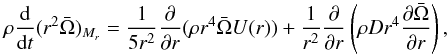 (2)where
  is the mean angular velocity on an isobaric surface, r the radius, ρ the density, Mr the mass inside the radius r, U the amplitude of the radial component of the meridional circulation2, and D the total diffusion coefficient in the vertical direction, taking into account the various instabilities that transport angular momentum. The first term on the right-hand side of this equation is the divergence of the advected flux of angular momentum, while the second term is the divergence of the diffused flux. The effects of expansion or contraction are automatically included in a Lagrangian treatment. The expression of U(r) (see Maeder & Zahn 1998) involves derivatives up to the third order; Eq. (2) is thus of the fourth order and implies four boundary conditions. These conditions are obtained by requiring momentum conservation and the absence of differential rotation at convective boundaries (Talon 1997). In particular, the boundary condition imposing momentum conservation at the bottom of the convective envelope has to take into account the impact of tides owing to the presence of the planet:
 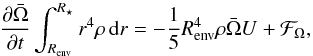 (3)with Renv the radius at the base of the convective envelope. ℱΩ represents the torque applied at the surface of the star. It is given here by
 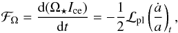 (4)where Ω⋆ is the angular velocity at the surface of the star and Ice is the moment of inertia of the convective envelope, ℒpl is the angular momentum of the planetary orbit, and (ȧ/a)t is the inverse of the timescale for the change of the orbit of the planet resulting from tidal interaction between the star and the planet. The expression of (ȧ/a)t is discussed below.
2.2. Physics of the evolution of the orbit
The evolution of the semi-major axis a of the planetary orbit, which we suppose to be circular (e = 0) and aligned with the equator of the star, is given by (see Zahn 1966, 1977, 1989; Alexander et al. 1976; Livio & Soker 1984b; Villaver & Livio 2009; Mustill & Villaver 2012; Villaver et al. 2014) ![Mathematical equation: \begin{equation} \left(\frac{\dot{a}}{a} \right)= \underbrace{-\frac{\dot{M}_{\star}+\dot{M}_{\rm pl}}{M_{\star}+M_{\rm pl}}}_{\rm Term\ 1} \underbrace{-\frac{2}{M_{\rm pl}v_{\rm pl}}\left[F_{\rm fri} + F_{\rm gra}\right]}_{\rm Term\ 2} \underbrace{-\left(\frac{\dot{a}}{a} \right)_{t}}_{\rm Term\ 3} , \label{equa:evoorb} \end{equation}](/articles/aa/full_html/2016/07/aa28044-15/aa28044-15-eq32.png) (5)where Ṁ⋆ = −Ṁloss with Ṁloss being the mass-loss rate (here given as a positive quantity). Mpl and Ṁpl are the planetary mass and the rate of change in the planetary mass, vpl is the velocity of the planet. Ffri and Fgra are, respectively, the frictional and gravitational drag forces, while (ȧ/a)t is the term that takes into account the effects of the tidal forces.
(5)where Ṁ⋆ = −Ṁloss with Ṁloss being the mass-loss rate (here given as a positive quantity). Mpl and Ṁpl are the planetary mass and the rate of change in the planetary mass, vpl is the velocity of the planet. Ffri and Fgra are, respectively, the frictional and gravitational drag forces, while (ȧ/a)t is the term that takes into account the effects of the tidal forces.
We do not discuss here the expressions of terms 1 and 2, since they are already extensively discussed in the references mentioned above. Here we focus on term 3, the tidal term, which is the term responsible for the exchange of angular momentum between the planet and the star, and in which the rotation of the star is explicitly involved.
When a convective envelope appears, tidal dissipation can be very efficient in the stellar envelope. As a result, angular momentum is transferred from the planetary orbit to the star or the inverse depending on whether the orbital angular velocity of the planet is smaller or larger than the axial angular rotation of the star. The term 3 is given by (Zahn 1966, 1977, 1989): 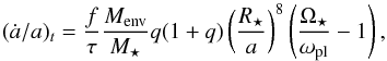 (6)with Menv the mass of the convective envelope, q = Mpl/M⋆, ωpl the orbital angular velocity of the planet, and Ω⋆ the angular velocity at the stellar surface. τ is the convective eddy turnover timescale and f is a numerical factor equal to the ratio of the orbit half period P/ 2 to the convective eddy turnover time f = (P/ 2τ)2 when τ>P/ 2 to consider the only convective cells that give a contribution to the viscosity; otherwise f is equal to 1 (Villaver & Livio 2009). The eddy turnover timescale is taken as in Rasio et al. (1996):
 ![Mathematical equation: \begin{equation} \tau=\left[\frac{M_{\rm env}(R-R_{\rm env})^{2}}{3L_{\star}} \right]^{1/3}\cdot \label{equa:tau} \end{equation}](/articles/aa/full_html/2016/07/aa28044-15/aa28044-15-eq49.png) (7)
(7)
2.3. The planet model
The frictional drag force depends on the radius of the planet. We assume that the planet/brown dwarf is a polytropic gaseous sphere of index n = 1.5 (Siess & Livio 1999a). We use the mass-radius relation by Zapolsky & Salpeter (1969). In our computations, we have taken into account for the first time the fact that the effective radius of the planet may be higher owing to a planetary magnetic field (Vidotto et al. 2014). We use the magnetic pressure radius given by  (8)where Bpl is the dipole’s magnetic field strength of the planet (Chapman & Ferraro 1930; Lang 2011). For Bpl we use the magnetic field of Jupiter at the equator, which is equal to 4.28 Gauss.
We find that the magnetic radius can be about a hundred times larger than the radius of the planet. This increases the frictional term by about 4 orders of magnitudes. However, even in this case, friction can only change the radius of the orbit by about one percent. Thus, the impact of the friction term remains small.
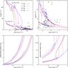 |
Fig. 1 Upper left panel: evolution of the surface equatorial velocity for our stellar models. No tidal interactions and planet engulfments are considered. The initial masses and rotations are indicated. The rectangle area indicated at the right bottom corner indicates the region that is zoomed on the upper right panel. Upper right panel: zoom on the RG branch phase for the same stellar models, as those shown on the upper left panel. Triangles indicate where the dredge-up occurs. Black full squares correspond to the sample of red giants observed by Carlberg et al. (2012). Lower left panel: evolution of the corotation radius (in au) for rotating stellar models with no tidal interactions during the RG branch phase. For the 2.5 M⊙, the core He-burning phase is also shown. The rectangle area indicated at the left bottom corner indicates the region that is zoomed on the lower right panel. Lower right panel: same as the lower left panel, but the MS phase and the crossing of the Hertzsprung-Russel (HR) gap are shown. |
2.4. Initial conditions considered
We consider stars with initial masses of 1.5, 1.7, 2, and 2.5 M⊙ and an initial rotation equal to Ωini/ Ωcrit = 0.1 and 0.5, where Ωini is the initial angular velocity on the ZAMS and Ωcrit the critical angular velocity on the ZAMS (i.e. the angular velocity such that the centrifugal acceleration at the equator balances the acceleration owing to the gravity at the equator).
The initial mass range considered in this work (M > 1.5 M⊙) contains relatively fast rotators (see next section) in contrast with lower initial mass stars (M < 1.5 M⊙). Indeed, stars above 1.5 M⊙ do not have a sufficiently extended outer convective zone to activate a dynamo during the main sequence so that, unless they host a fossile magnetic field, they do not undergo any significant magnetic braking. Presently, only a small fraction of these stars (of the order of 5−10%, see the review by Donati & Landstreet 2009, and references therein) host a surface magnetic field between 300 G and 30 kG. Lower initial mass stars have an extended outer convective zone during the main sequence and thus activate a dynamo and experience a strong braking of the surface by magnetized winds. The physics of these lower initial mass stars is therefore different and will be the topic of another paper in this series.
A metallicity of Z = 0.02 has been chosen to account for the fact that the mean metallicity of the current sample of planet-host stars is slightly higher than solar (Santos et al. 2001, 2004; Sousa et al. 2011) and so it is the metallicity of the RG stars known to host planets in the mass range under study (Maldonado et al. 2013; Maldonado & Villaver 2016). Planets with masses equal to 1, 5, 10, and 15 Jupiter masses (MJ) have been considered. The initial semi-major axes (a0) have been taken in the range [0.35−4.5] au. The eccentricities of the orbits are fixed to 0. The computations were performed until the He-flash (tip of the RG branch) for the 1.5, 1.7, and 2 M⊙, and until the end of the core He-burning phase for the 2.5 M⊙ 3.
3. Rotating stellar models without tidal interactions
It is important to study the evolution of single rotating stars to reveal, by contrast, the differences that appear when tidal interactions with a planet are occurring. In this section, we first describe how the surface velocity of a single star evolves from the main-sequence (MS) phase up to the tip of the RG branch. We then discuss how the corotation radius evolves, because this quantity plays a key role to determine in which direction the angular momentum is transferred, from the orbit to the star or from the star to the orbit. Finally, we study how rotation, by changing the global and internal properties of the star, has an impact on the tidal forces and hence on the evolution of a planetary orbit, and of its own rotation.
3.1. Evolution of the surface rotation for isolated stars
The upper left panel of Fig. 1 shows the evolution of the equatorial surface velocity from the ZAMS until the tip of the RG branch or the end of the core He-burning phase (for the 2.5 M⊙) for stellar models without any tidal interactions. We see that our slow rotating models (Ωini/ Ωcrit = 0.1) correspond to surface rotations during the MS phase around 20 km s-1, while our fast rotating models (Ωini/ Ωcrit = 0.5) correspond to surface velocities around 100−110 km s-1.
Zorec & Royer (2012) analysed the vsini for a sample of more than two thousand B6- to F-type stars. They find that for stars with masses between about 1.6−2.5 M⊙, the velocity distribution is unimodal, with Maxwellian distributions that peak between 160 and 180 km s-1. The adopted rotation rates are thus in the low range of observed velocities. We focus on this low range of rotations for mainly the following reason: stars with planets might show slower initial rotations than stars without planets, since the angular momentum of the protostellar cloud has to be shared between the planets and the star instead of being locked in only the star. Of course, many processes may evacuate the angular momentum of the cloud, planet formation being only one of them. Nevertheless, it appears reasonable to think that stars with planets might initially rotate slower than stars without planets (Bouvier 2008).
The upper right panel of Fig. 1 shows that along the RG branch the surface velocity drops to lower and lower values when the surface gravity decreases. The bulk of red giants observed by Carlberg et al. (2012) are characterized by initial masses (estimated from their positions in the HR diagram) between 1.3 and 3 M⊙. They are well framed by our slow and fast rotating models despite the fact that, as discussed just above, our initial rotations span only a subset of the range of values shown by the progenitors of red giants. This mainly arises from the fact that the inflation of the star during the RG phase is so large that many different initial surface rotations on the ZAMS converge to similar values at that stage. We also see that, to explain the slow observed rotation of the bulk of the red giant stars, there is a priori no need to invoke any magnetic braking that would be activated when the convective envelope appears.
The big triangles along the tracks indicate where the dredge-up occurs. No surface acceleration is observed at that point. Therefore, our models do not confirm the idea suggested by Simon & Drake (1989) that a short-lived rapid rotation phase during the RG phase occurs when the deepening stellar convection layer dredges up angular momentum from the more rapidly rotating stellar interior. Actually, some angular momentum is indeed dredged-up from the core to the surface, but the central region of the star is so compact and its moment of inertia so small that, even if the core rotates fast, its angular momentum is quite small with respect to the angular momentum of the envelope. Thus, this dredge-up has a negligible impact on the surface rotation of red giants.
Finally, we note that among the 17 red giants with a vsini above 8 km s-1, about seven (those at the base of the RG branch in the vicinity of the Ωini/ Ωcrit = 0.5 tracks) might be explained without any particular acceleration mechanism. Of course, vsini is a lower limit to the true equatorial surface velocity and thus among these stars a few stars can still be much more rapid rotators but, without any other pieces of information, these surface velocities cannot be considered as strong evidence of tidal interaction with a planet or a brown dwarf, or resulting from an engulfment. Stronger candidates are those RGs that are well above the tracks. These best candidates are not located at the base of the RG branch. This differs from conclusions obtained in previous works, where it was suggested that the rapid rotation signal from ingested planets is most likely to be seen on the lower RG branch (Carlberg et al. 2009). Also the present results show that the use of a fixed lower limit for vsini around 8 km s-1 does not appear very adequate to characterize red giants that are candidates for tidal interaction with a planet or a brown dwarf, or resulting from an engulfment. This limit clearly depends on the surface gravity for a given initial mass star.
3.2. Evolution of the corotation radius
The corotation radius corresponds to the orbital radius for which the orbital period would be equal to the rotation period of the star. When the actual distance of the planet to the star is inferior to the corotation radius, tidal forces reduce the orbital radius, while when the actual distance of the planet to the star is larger, tidal forces enlarge the orbital radius. This is accounted for in Eq. (6) through the term  .
.
The two lower panels of Fig. 1 show the evolution of the corotation radius ( ) for various rotating models (without planets). The lower right panel shows the situation during the MS phase and the crossing of the HR gap, while the lower left panel shows the evolution along the RG branch (and in case of the 2.5 M⊙ also during the core He-burning phase).
To have an engulfment, a necessary condition (but of course not a sufficient one) is that the actual radius of the planetary orbit is inferior to the corotation radius. For an engulfment to occur, the tidal forces need to be of sufficient amplitude when the orbital radius is smaller than the corotation radius.
The corotation radius is very small during the MS phase. Even in case where tidal dissipation would be efficient at that stage, tidal forces can only decrease the radius of the orbit when the distance is below 0.05-0.15 au if the star has a quite low initial rotation rate (Ωini/ Ωcrit = 0.1). If the star is initially rotating rapidly (Ωini/ Ωcrit> 0.5), in the case of the 2 M⊙, the corotation radius is inferior to 0.01 and 0.03 au during the MS phase4.
Along the RG branch, the corotation radius increases a lot as a result of the decrease of the surface rotation rate. The corotation radii are shifted downwards when the initial rotation rate increases, as was the case during the MS phase.
The initial distances between the planet and the star considered in this work are clearly above the corotation radius during the MS phase, will cross it, and thus become inferior to it during the red giant branch. Since the rotation of the star is modified because of the tidal interaction, we shall have to see how the corotation radius changes as a result of this interaction (see Sect. 4.3).
3.3. Impact of rotation on the structure and the evolution of the star
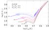 |
Fig. 2 Evolutionary tracks in the Hertzsprung-Russell diagram for rotating models of 1.5, 1.7, 2.0, and 2.5 M⊙. The solid and dashed lines indicate models with Ωini/ Ωcrit = 0.1 and 0.5, respectively. |
In Fig. 2, the evolutionary tracks in the HR diagram of our stellar models are shown. Differences between rotating models for a given mass appear mainly during the MS phase and during the crossing of the HR gap. Faster rotating models are overluminous at a given mass and the MS phase extends to lower effective temperatures. The widening of the MS is mainly due to the increase of the convective core that is related to the transport by rotational mixing of fresh hydrogen fuel in the central layers. The impact on the luminosity results from both the increase of the convective core and the transport of helium and other H-burning products into the radiative zone (e.g. Eggenberger et al. 2010; Maeder & Meynet 2012). The increase of the convective core also leads to an increase of the MS lifetime. Typically, faster rotating models will reach a given luminosity along the RG branch at an older age than the slower rotating models.
Along the RG branch, at a given effective temperature, the initially fast rotating track is slightly overluminous with respect to the slow one. This means that the radius of the fast rotating star is also larger than the radius of the slow one. The tidal forces will therefore be stronger around the fast rotating star (the tidal force varies with the stellar radius at the power 8) and we may expect that, everything being equal, when an engulfment occurs, it will occur at an earlier evolutionary stage (typically at smaller luminosities along the RGB) around fast rotating stars than around slow rotating ones. We note that since rotation increases the MS lifetime, a given evolutionary stage along the RGB occurs at a greater age when rotation increases. We also note that the tip of the RG branch occurs at slightly lower luminosities for the faster rotating models (see Fig. 2). This implies that the maximum radius reached by the star decreases when the initial rotation of the star increases. Therefore, increasing the stellar rotation slightly lowers the maximum initial distance between the star and the planet that leads to an engulfment5.
The decrease in luminosity at the tip comes from the fact that the mass of the core at He-ignition in the 2 M⊙ with Ωini/ Ωcrit = 0.5 is smaller than in the same model with Ωini/ Ωcrit = 0.1. At first sight, it might appear strange that the core mass is smaller in the faster rotating model. Indeed, rotation, in general, makes the masses of the cores larger. The point to keep in mind here is that we are referring to the mass of the core required to reach a given temperature, which is the temperature for helium ignition. This mass depends on the equation of state. In semi-degenerate conditions, the core mass needed to reach that temperature is larger than in non-degenerate ones (see, e.g. Fig. 14 in Maeder & Meynet 1989). For a given initial mass, faster rotation, by increasing the core mass during the core H-burning, makes the helium core less sensitive to degeneracy effects. In other words, rotation shifts the mass transition between He-ignition in semi-degenerate and non-degenerate regimes to lower values.
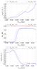 |
Fig. 3 Top: evolution of stellar radii for the 2 M⊙ models. Continuous and dotted lines correspond to stars with initial velocities Ωini/ Ωcrit = 0.1 and 0.5, respectively. Time 0 corresponds to the end of the MS phase. Centre: evolution of the total mass of the star (upper red lines) and of the masses of the convective envelopes (lower blue curves) for the same stars as in the top panel. Bottom: radii at the bottom of the convective envelopes for the same stars as in the top panel. |
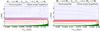 |
Fig. 4 Left panel: evolution of the semi-major axis of a 1 MJ planet orbiting a 2 M⊙ star, computed with an initial rotation on the ZAMS of Ωini/ Ωcrit = 0.1. The different lines correspond to different initial semi-major axis values. Only the evolutions in the last 50−60 million years are shown. Before that time, the semi-major axis remains constant. The red solid lines represent the planets that will be engulfed before the star has reached the tip of the RG branch; the blue dashed lines represent the planet that will avoid the engulfment during the RG branch ascent. The upper envelope of the green area gives the value of the stellar radius. Right panel: same as the left panel, but for an initial rotation Ωini/ Ωcrit = 0.5. |
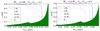 |
Fig. 5 Left panel: evolution of the orbit for planets of masses equal to 1 MJ (blue solid line), 5 MJ (black dotted line), 10 MJ (red dashed line) and 15 MJ (magenta dashed-dotted line) around a 2 M⊙ star with an initial rotation equal to 10% the critical angular velocity. The initial semi-major axis is equal to 0.5 au. Right panel: same as the left panel, but for an initial rotation rate equal to 50% of the critical angular velocity. |
The evolution of the radius as a function of time along the RG branch in the case of the 2 M⊙ models is shown in Fig. 3 (top panel). The radius at the tip of the RG branch is lower by about 0.1 dex, therefore by 25% in the case of the faster rotating model. The small bump seen along the curves at time coordinates 0.06 and 0.075 is due to the fact that, when the star climbs the RG branch, the H-burning shell moves outwards in mass and, at a given point, encounters the chemical discontinuity left by the convective envelope that also slowly recedes outwards after the first dredge-up. This produces a rapid increase in the abundance of hydrogen in the H-burning shell, a variation in the energy output of this shell, and a change in the structure that produces these bumps.
Center and bottom panels of Fig. 3 show how the masses and the radii at the base of the convective envelope vary as a function of time in both rotating models. In the faster rotating model, the convective envelope has a slightly smaller extension in mass and radius than in the slower rotating model. However these changes are minor.
From this brief discussion, we can conclude that rotation, by changing the transition mass between stars going through an He-flash and those avoiding it, may have a non-negligible impact on the orbital evolution in this mass range. Outside this mass range, the impact of rotation will be modest.
4. Planetary orbit evolution and stellar rotation
4.1. Planetary orbit evolution
In Fig. 4, we compare the evolution of the semi-major axis for planets of 1 MJ orbiting around 2 M⊙ stars with an initial slow and rapid rotation on the ZAMS. As previously obtained by many authors (see e.g. Kunitomo et al. 2011; Villaver & Livio 2009; Villaver et al. 2014), and as recalled in the previous section, the evolution of the orbit for planets that are engulfed is a kind of runaway process. Once the tidal forces begin to play an important role, a rapid decrease of the radius of the orbit is observed as a result of the very strong dependency of the tidal force on the ratio between the stellar radius that is increasing and the semi-major axis that is decreasing (term in (R∗/a)-8 in Eq. (6)). Comparing the left and the right panel of Fig. 4, we see that the interval of initial distances leading to an engulfment during the RG branch is a bit smaller for the faster rotating models (see the change of the limit between the continuous red and the dashed blue lines). As explained in Sect. 3 above, the larger the initial rotation rate, the lower the luminosity at the RG tip. A lower luminosity leads to a lower value for the maximum stellar radius, and thus to more restricted conditions for an engulfment.
Figure 5 shows the impact of different initial rotation rates for a 2 M⊙ on the orbital decay of planets of various masses beginning all their evolution at a distance equal to 0.5 au. The orbit for the 15 MJ planet, for instance, presents a different evolution around the slow and the fast rotator. The orbital decay occurring around the slow rotating star (magenta dashed-dotted line on the left panel) only occurs during the bump. The decrease of the semi-major axis slows down when the stellar radius decreases since the tidal force depends on (R∗/a)-8. Around the fast rotating model (see the magenta dashed-dotted line on the right panel), the orbit decay only occurs at the beginning of the bump and is quite rapid. As mentioned above, this illustrates that stellar rotation changes the structure of the star and thereby modifies the evolution of the orbit. In general, the engulfment occurs at an earlier evolutionary stage when the initial rotation rate increases.
4.2. Impact of stellar rotation on the conditions leading to an engulfment
As already discussed in the literature (see e.g. Villaver & Livio 2009; Villaver et al. 2014), we see that, for a given mass of the planet and for given properties of the host star, a maximum initial semi-major axis exists, below which engulfment will occur during the RG phase. These maximal values are given in Table 1 and shown in Fig. 6. These results illustrate that the conditions for engulfment are more restricted around fast rotating stars, but the effect remains quite modest for the 1.5 and 2.5 M⊙ models, while it is more significant for the intermediate mass cases for the reasons already explained above.
Initial semi major axes below which the planet is engulfed during the RG phase.
In Fig. 6, we note that the effects of rotation do not produce overlaps between the curves, indicating that the change that is due to the initial mass dominates over the change that is due to rotation (at least for the range of rotation rates considered here). The present results for the evolution of planetary orbits are well in line with previous works (Kunitomo et al. 2011; Villaver & Livio 2009; Villaver et al. 2014). More specifically, we also obtain that the conditions for engulfment are more favorable for more massive planets and less massive stars (we note that this is because the less massive stars reach larger luminosities at the tip of the RGB). Moreover, Kunitomo et al. (2011) find that the orbital radius above which planet engulfment is avoided is quite sensitive to the stellar mass at the transition between those going through a helium flash and those avoiding the helium flash. Qualitatively, this is exactly what we find here (see Fig. 6).
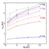 |
Fig. 6 Variation of the maximum semi-major axis below which engulfment occurs during the RG ascent as a function of the mass of the planet, of the mass of the star, and its initial rotation rate. The dashed and continuous lines are, respectively, for an initial stellar angular velocity equal to 10% and 50% of the critical one. The empty symbols connected by light dashed-dotted lines are the results obtained by Villaver et al. (2014) for planets with masses of 1, 2, 5, and 10 MJ orbiting a non-rotating 1.5 M⊙ star. The triangles are for models using weak mass loss rates during the red giant phase (η = 0.2 in Eq. (1)), the circles are for models with normal RG mass losses (η = 0.5), and the squares are for models with η = 0.5 and overshooting. |
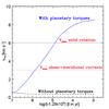 |
Fig. 7 Evolution of the equatorial velocity at the surface of a 2 M⊙. The dashed line corresponds to the evolution obtained from a model with an initial surface angular velocity equal to 10% of the critical angular velocity without tidal interaction. The continuous line corresponds to the same model but accounting for the transfer of angular momentum from the planetary orbit to the star (15 MJ planet beginning to orbit at 1 au on the ZAMS). The line stops at engulfment. The two horizontal dotted lines indicate the maximum velocities that can be produced in some extreme situations from single stars at the position in the HR diagram where engulfment occurs. The lowest limit corresponds to models computed with the same physics of rotation as here but starting from a much higher initial rotation equal to about 95% the critical rotation on the ZAMS. The upper limit would correspond to a model starting with the same very high initial velocity, assuming solid-body rotation during its whole evolution. |
In Fig. 6, we have also plotted the semi-major axis above which no engulfment occurs (survival limit) predicted by Villaver et al. (2014) for planets with masses between 1, 2, 5, and 10 MJ around a non-rotating 1.5 M⊙ computed with different physical ingredients (see caption). The upper curve from Villaver et al. (2014) was obtained with a smaller mass loss rate during the ascent of the RG branch. Lowering the mass loss rate leads to larger radii at the tip of the RG branch and thus shifts the survival limit to larger values. The two lower curves by Villaver et al. (2014) use the same mass loss rates as in the present work. The two curves differ by the inclusion of overshooting, the lower curve (empty squares) being the one computed with overshooting. This last model would likely be the one that is the most comparable with the present models, although there are differences (for instance the chemical composition is different). In any case, the differences are small and we note that increasing the core size slightly shifts the curve downward as in the present models. Interestingly, we note that mass losses along the RG branch likely has a larger effect than rotation for this specific initial mass.
4.3. Impact of the orbital decay on the stellar rotation
When the semi-major axis of the planetary orbit is inferior to the corotation radius, the tidal forces can transfer angular momentum from the orbit of the planet to the star, accelerating its rotation. The question we want to address here is whether this would produce some observational effects before the engulfment6. We can wonder whether this type of transfer can lead to high surface velocities at the stellar surface that would be difficult to explain by any other mechanism. If yes, we then have to investigate whether these velocities are reached for a sufficiently long period to be observable. We can begin by considering a few orders of magnitude. From Tables and , we see that the angular momentum contained in the orbit ranges between 1 and 46 times the angular momentum contained in the star (see third column). Thus we can expect that the transfer of even half of this angular momentum will have a significant impact on the angular momentum of the star. Due to the orbital decay, the planet will lose a significant part of its angular momentum (see the amount of the initial orbital angular momentum lost by the orbital decay in Col. 9). At the moment of engulfment, the planet therefore has an angular momentum, which is only a fraction of its initial value (the angular momentum at time of engulfment is given in Col. 8). Of course the sum of the fraction given in Cols. 8 and 9 gives 1.
Only part of the orbital angular momentum lost by the planet is transferred to the star, the part that is due to the tidal forces. The part of the orbital decay that is due to the other processes (stellar winds, changes of the planet mass, friction, and gravitational drag forces) do not transfer any angular momentum from or to the star (the fraction of the angular momentum lost by these processes is indicated in Col. 10 as a fraction of Col. 9). We then obtain the amount (in percents) of the initial orbital angular momentum transferred to the star by ℒmigr(1−fnotides/ 100) ~ ℒmigr. This amount is, in general, more than half of the initial orbital angular momentum in agreement with previous estimates (Carlberg et al. 2009). In the case of the 2 M⊙ star with Ω/Ωcrit = 0.1 and a 15 MJ planet beginning to orbit at 1 au on the ZAMS, the angular momentum transferred from the orbit to the star is equivalent to more than 22 times the angular momentum contained in the convective outer envelope. This implies that the angular velocity of the star is enhanced by a factor of about 23 as well as the surface velocity, which will increase from 0.47 km s-1 to 10.8 km s-1. Actually, this process does not occur instantaneously and during the transfer the structure of the star changes, and thus the real increase will be less than the one obtained from this simple estimate.
In Fig. 7, we show how the surface velocity of the star increases owing to the orbital decay in the case of the 2 M⊙ with Ω/Ωcrit = 0.1, and a 15 MJ planet beginning to orbit at 1 au on the ZAMS. We see that the whole acceleration process takes place in less than 10 Myr. This duration corresponds to about 17% of the RG branch ascent phase, which is not negligible, and indicates that it is not unreasonable to observe systems that are in this type of phase. Before the engulfment, the period during which the surface velocity would be larger than 6 and 8 km s-1 would be respectively two and three orders of magnitude shorter (i.e. of the order of 100 000 yr and 10 000 yr, respectively). The duration of these phases of high surface rotation rates before engulfment, although not negligible, are respectively only 2 thousandths or 2 ten thousandths of the RG branch duration, and are therefore much more difficult to observe. As we shall see in the second paper of this series, these high velocities will be maintained for long periods after engulfment, indicating that high velocity red giants will be more easily observed after engulfment than just before.
In Fig. 7, we have also indicated the values of the surface velocity reached by a 2 M⊙ star at the same position in the HR diagram as that where the engulfment occurs, but assuming that the star started with a very high initial rotation rate on the ZAMS equal to 95% the critical velocity. The star is assumed to evolve as a single star without planet engulfment or any other interaction. We see that such an evolution cannot predict surface rotation rates beyond a velocity of about 3 km s-1. Of course the surface velocity depends on the way angular momentum is transported inside the star. The values shown in Fig. 7 have been obtained with the physics presented in Sect. 2. If we assume that stars rotate as solid bodies, then we would obtain the limit shown by the upper dotted line. Even in this case, the velocities remain below 6 km s-1. This indicates that surface velocities for red giants above a value of 6 km s-1 and for a surface gravity log g ~ 1.5 cannot be obtained for single stars. Such a high surface velocity for a red giant with a low surface gravity is the signature of an interaction.
We end this section by comparing the kinetic energy of the planet just before engulfment with the binding energy of the convective envelope (see Cols. 11 and 13 in Tables and ). We see that the kinetic energy is two to three orders of magnitude smaller than the binding energy, thus it is not expected that any stripping off of the envelope will occur as a result of injection into the convective envelope of the kinetic energy of the planetary orbit. We note also that the enhancement of the rotation rate at the surface would not be able to make the star reach the critical velocity. Indeed, we have just seen above that the velocity reaches values of the order of 10 km s-1, while the critical velocity along the RG branch for a 2 M⊙ star is of the order of 100 km s-1.
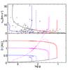 |
Fig. 8 Upper panel: evolution of the surface equatorial velocity for various 2 M⊙ models with and without planets. The continuous black curves are for models without planets. The lower curve is for the models with Ωini/ Ωcrit = 0.1, the upper curve for Ωini/ Ωcrit = 0.5. The coloured curves are for models with planets. The evolution is shown only until the engulfment. The continuous (dashed) curves correspond to Ωini/ Ωcrit = 0.1 (Ωini/ Ωcrit = 0.5) models. The planets have a mass equal to 15 MJ. From left to right, we show the case for an initial distance between the star and the planet equal to 0.5, 1.0 and 1.5 au. Lower panel: evolution of the semi-major axis of the planetary orbit (coloured continuous and dashed curves) and the evolution of the stellar radii (black lower curves). The long-short dashed (magenta) curve shows the evolution of the corotation radius for the 2 M⊙ with Ωini/ Ωcrit = 0.5 without planet, the dotted line for the same model with a tidal interaction with a 15 Mj planet beginning its orbital evolution at a distance of 1 au from the star. The curve stops at engulfment. |
4.4. Comparisons with observed systems
In the upper panel of Fig. 8, we compare the surface velocities obtained for our 2 M⊙ models with and without tidal interactions with the observed sample of red giant stars observed by Carlberg et al. (2012). The results of the present work show that the most clear candidates for a tidal interaction (see the points above the track for the fast rotating single star model) are those red giants located near the end of the RG branch, i.e. for log g< 2.5. The velocities obtained by models with tidal interactions can reach values equal or even above those that would be needed to reproduce these fast rotating red giants. While some of these red giants might still be in a stage before an engulfment (for instance those with vsini = 3−5 km s-1 at log g below 1.4), others (those with vsini around 14 km s-1 with log g between 1.9 and 2.4) are more likely red giants that have evolved after a tidal interaction/engulfment. Indeed, the duration of the rapid increase of the surface velocity before the engulfment is so short that there is little chance to observe stars at that stage; there is, however, more chance to observe stars after the engulfment.
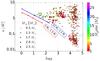 |
Fig. 9 Semi-major axis of planetary orbits versus the surface gravity (log g) of the host stars using the database of exoplanets.org (Han et al. 2014) and of NASA Exoplanet Archive (Akeson et al. 2013). The colours enable us to have an indication of the mass of the planet, while the size of the symbols are related to the mass of the star. The thick lines in the upper left corner show the minimum semi-major axis for survival of the planet as computed in the present work for stars with Ωini/ Ωcrit = 0.10. The case for Ωini/ Ωcrit = 0.50 would be barely distinguishable. These lines are labelled by the masses of the planet and of the star considered. |
In the lower panel of Fig. 8, the evolution of the corresponding orbits of 15 MJ planets are shown. The evolution of the corotation distance is also shown for a 2 M⊙ model with (magenta dotted line) and without a planet (magenta short-long dashed curve). The corotation distance decreases when the star accelerates as a result of the tidal acceleration (see the dotted magenta line in Fig. 8), however, the orbital radius always remains interior to the corotation radius and thus an engulfment occurs.
Another interesting plot to check whether the theoretical predictions are compatible with current observations is the one shown in Fig. 9, where the semi-major axis of planets of various masses are plotted as a function of the gravity of the star. The most striking fact is that one can observe planets with much smaller semi-major axis around main-sequence stars, i.e. with log g larger than 4, than around evolved stars, i.e. with log g smaller than about 3.0 (see e.g. Kunitomo et al. 2011). Typically, for stars with log g smaller than about 3.0, no planets with a semi-major axis inferior to about 0.5 au are observed. This might reflect the fact that planets with smaller semi-major axis are engulfed by the star.
From the present computations, on that diagram we can plot the gravity at which engulfment occurs on the RG branch for different initial semi-major axis. In the case of 1 MJ planets around 1.5 M⊙ stars, we obtain the thick red lines. For 15 MJ planets, we obtain the thick blue line. The results are obtained for the initially slow rotating stellar models. The case for the fast rotating model is barley distinguishable in Fig. 9. According to present computations, we should barely observe any systems with smaller semi-major axis than those given by these lines at the considered gravities. We see that indeed, for the systems considered in this work, all observed systems have semi-major axis that are larger than the predicted limits.
Some gaps, however, seem to remain between the theoretical limits obtained here and the observations. At the moment, it is difficult to know whether this type of gap really exists or not, since a careful study of the observational biases would be required. This type of gap, if real, might indicate that the true survival limit could still be larger than the one predicted here.
We end this section with a few comments about the frequency of planet engulfments. If we first consider the case of 1 MJ planets around 2 M⊙ stars. We can assume that the survival limit is 1.5 au (an intermediate value between 1.4 and 1.7 au indicated in Table 1), that there are Jupiter-like planets around a fraction f of stars, and that the probability for these planets to be at distance a and a + da from its parent star is given by  with amax the maximum initial radius of the orbits of such planets, we obtain the probability of planet engulfment to be
  . If we set f ~ 1, asurvival = 1.5 and amax = 10, we obtain a probability equal to 2.25%. The hypotheses done are very schematic and are likely not very realistic. It is even difficult to say whether the result obtained is an upper or a lower limit. Nevertheless, it already provides interesting information, namely that if the distances at birth are uniformly distributed, then one expects about one percent of 2 M⊙ red giants to engulf a planet. This number will be slightly larger for lower-mass stars and slightly smaller for more massive stars.
5. Conclusions
In this paper, we studied the evolution of the orbits of planets with masses between 1 and 15 MJ around stars with masses between 1.5 and 2.5 M⊙.
The originality of the present work lies in the fact that we used rotating stellar models enabling us to study for the first time the impact of the stellar rotation on the evolution of the planetary orbit, as well as the feedback of the evolution of the planetary orbit onto the rotation of the star itself. The main results are the following:
-
The present rotating stellar models enable us to study the range of surface rotations expected along the RG branch for stars evolving without tidal interactions. For stars with initial masses below 2.5 M⊙, whatever the initial rotation, the surface velocities are smaller than 5 km s-1 for surface gravities in log g below 2. We note that the first dredge-up does not produce any significant surface acceleration.
-
The surface velocity limit separating the normal rotating red giants (no tidal interaction) from red giants whose surface velocities, by way of explanation, require some acceleration mechanism that depends on the mass of the star and on its surface gravity. For instance, for a 2.5 M⊙ star, this limit is around 15 km s-1 for a log g equal to 2.6 and equal to 2 km s-1 for a log g equal to 1.
-
The best candidates of red giants having been accelerated by tidal interactions with a companion (and possibly also by an engulfment of a companion) need to be searched for in the upper part of the RG branch, where stellar models predict surface velocities below 5 km s-1, even starting from very high initial rotation rates.
-
The orbital decay occurs at earlier evolutionary stages in faster rotating models. This is a consequence of the changes of the structure of the star due to rotation, in particular the fact that rotating stars are slightly overluminous and thus have a larger radius at a given effective temperature.
-
The survival domain of planets around stars, which initially rotate fast, are more restricted than the survival domain of planets around stars that initially rotate slowly. This survival limit is the most sensitive to the initial rotation in the mass range around the mass for He-flash (this transition is between 2 and 2.5 M⊙ according to the present models). In this domain, passing from a low initial angular velocity, which is equal to 10% of the critical value to 50%, decreases the minimum semi-major axis for survival by about 20%. Outside this mass range, the impact of rotation is more modest. We note that, in the helium flash transition domain, the survival limit also depends sensitively on other parameters, such as the core overshooting or the metallicity.
-
The surface rotation of the star begins to increase before the engulfment (typically a few 105 years before in the case of our 2 M⊙ model with Ωini/ Ωcrit = 0.1 and a 15 MJ planet beginning to orbit at 1 au on the ZAMS) and can be enhanced by factors between 10 and 20. These velocities are still well below the critical velocity, and well below the value that would be needed for the corotation radius to be smaller than the actual radius of the orbit, and thus make the tidal forces reverse their direction and the planet follow an outward migration. High surface velocities (typically higher than 10 km s-1) will be reached only during very short periods before engulfment. As we shall see in the second paper of this series, pursuing the evolution of the star beyond engulfment shows that the high velocities reached by tidal interactions and by the engulfment itself will not disappear in short timescales and can produce fast rotating red giants.
In their footnote 2, Carlberg et al. (2009) write: “Rotation also plays an important role; however, grids of evolution models explicitly accounting for rotational effects are not currently available for the range of stellar masses in our study”.
The radial component u(r,θ) of the velocity of the meridional circulation at a distance r to the centre and at a colatitude θ can be written u(r,θ) = U(r)P2(cosθ), where P2(cosθ) is the second Legendre polynomial. Only the radial term U(r) appears in Eq. (2).
This model ignites helium in a non-degenerate regime; there is therefore no helium flash.
As discussed above, we do not expect frequent magnetic braking during the MS phase since these stars, having no extended outer convective envelope, do not present any efficient dynamo activity.
Indeed, the larger the maximum stellar radius, the stronger the tidal forces and thus the larger the range of initial distances between the star and the planet that leads to an engulfment.
The case of the engulfment is treated in the second paper of the series.
Acknowledgments
This research has made use of the Exoplanet Orbit Database and the Exoplanet Data Explorer at exoplanets.org. The project has been supported by Swiss National Science Foundation grants 200021-138016, 200020-15710 and 200020-160119. A.A.V. acknowledges support from an Ambizione Fellowship of the Swiss National Science Foundation.
References
- Adamów, M., Niedzielski, A., Villaver, E., Nowak, G., & Wolszczan, A. 2012, ApJ, 754, L15 [NASA ADS] [CrossRef] [Google Scholar]
- Akeson, R. L., Chen, X., Ciardi, D., et al. 2013, PASP, 125, 989 [NASA ADS] [CrossRef] [Google Scholar]
- Alexander, M. E., Chau, W. Y., & Henriksen, R. N. 1976, ApJ, 204, 879 [NASA ADS] [CrossRef] [Google Scholar]
- Bear, E., & Soker, N. 2011, MNRAS, 414, 1788 [NASA ADS] [CrossRef] [Google Scholar]
- Bouvier, J. 2008, A&A, 489, L53 [NASA ADS] [CrossRef] [EDP Sciences] [Google Scholar]
- Carlberg, J. K. 2014, AJ, 147, 138 [NASA ADS] [CrossRef] [Google Scholar]
- Carlberg, J. K., Majewski, S. R., & Arras, P. 2009, ApJ, 700, 832 [Google Scholar]
- Carlberg, J. K., Smith, V. V., Cunha, K., Majewski, S. R., & Rood, R. T. 2010, ApJ, 723, L103 [NASA ADS] [CrossRef] [Google Scholar]
- Carlberg, J. K., Majewski, S. R., Patterson, R. J., et al. 2011, ApJ, 732, 39 [Google Scholar]
- Carlberg, J. K., Cunha, K., Smith, V. V., & Majewski, S. R. 2012, ApJ, 757, 109 [NASA ADS] [CrossRef] [Google Scholar]
- Chapman, S., & Ferraro, V. C. A. 1930, Nature, 126, 129 [NASA ADS] [CrossRef] [Google Scholar]
- Donati, J.-F., & Landstreet, J. D. 2009, ARA&A, 47, 333 [NASA ADS] [CrossRef] [MathSciNet] [Google Scholar]
- Eggenberger, P., Meynet, G., Maeder, A., et al. 2008, Ap&SS, 316, 43 [NASA ADS] [CrossRef] [Google Scholar]
- Eggenberger, P., Miglio, A., Montalban, J., et al. 2010, A&A, 509, A72 [NASA ADS] [CrossRef] [EDP Sciences] [Google Scholar]
- Ekström, S., Georgy, C., Eggenberger, P., et al. 2012, A&A, 537, A146 [NASA ADS] [CrossRef] [EDP Sciences] [Google Scholar]
- Fekel, F. C., & Balachandran, S. 1993, ApJ, 403, 708 [NASA ADS] [CrossRef] [Google Scholar]
- Han, E., Wang, S. X., Wright, J. T., et al. 2014, PASP, 126, 827 [NASA ADS] [CrossRef] [Google Scholar]
- Kunitomo, M., Ikoma, M., Sato, B., Katsuta, Y., & Ida, S. 2011, ApJ, 737, 66 [NASA ADS] [CrossRef] [Google Scholar]
- Lang, K. 2011, The Cambridge Guide to the Solar System (Cambridge University Press) [Google Scholar]
- Livio, M., & Soker, N. 1984a, MNRAS, 208, 783 [NASA ADS] [Google Scholar]
- Livio, M., & Soker, N. 1984b, MNRAS, 208, 763 [NASA ADS] [CrossRef] [Google Scholar]
- Maeder, A., & Meynet, G. 1989, A&A, 210, 155 [NASA ADS] [Google Scholar]
- Maeder, A., & Meynet, G. 2012, Rev. Mod. Phys., 84, 25 [NASA ADS] [CrossRef] [Google Scholar]
- Maeder, A., & Zahn, J.-P. 1998, A&A, 334, 1000 [NASA ADS] [Google Scholar]
- Maldonado, J., & Villaver, E. 2016, A&A, 588, A98 [NASA ADS] [CrossRef] [EDP Sciences] [Google Scholar]
- Maldonado, J., Villaver, E., & Eiroa, C. 2013, A&A, 554, A84 [NASA ADS] [CrossRef] [EDP Sciences] [Google Scholar]
- Massarotti, A., Latham, D. W., Stefanik, R. P., & Fogel, J. 2008, AJ, 135, 209 [NASA ADS] [CrossRef] [Google Scholar]
- Mustill, A. J., & Villaver, E. 2012, ApJ, 761, 121 [NASA ADS] [CrossRef] [Google Scholar]
- Nordhaus, J., & Spiegel, D. S. 2013, MNRAS, 432, 500 [NASA ADS] [CrossRef] [Google Scholar]
- Nordhaus, J., Spiegel, D. S., Ibgui, L., Goodman, J., & Burrows, A. 2010, MNRAS, 408, 631 [NASA ADS] [CrossRef] [Google Scholar]
- Rasio, F. A., Tout, C. A., Lubow, S. H., & Livio, M. 1996, ApJ, 470, 1187 [NASA ADS] [CrossRef] [Google Scholar]
- Reimers, D. 1975, Mémoires of the Société Royale des Sciences de Liège, 8, 369 [Google Scholar]
- Sackmann, I.-J., Boothroyd, A. I., & Kraemer, K. E. 1993, ApJ, 418, 457 [NASA ADS] [CrossRef] [Google Scholar]
- Santos, N. C., Israelian, G., & Mayor, M. 2001, ArXiv e-prints [arXiv:astro-ph/0109018] [Google Scholar]
- Santos, N. C., Israelian, G., & Mayor, M. 2004, VizieR Online Data Catalog: J/A+A/415/1153 [Google Scholar]
- Sato, B., Toyota, E., Omiya, M., et al. 2008, PASJ, 60, 1317 [NASA ADS] [Google Scholar]
- Siess, L., & Livio, M. 1999a, MNRAS, 304, 925 [NASA ADS] [CrossRef] [Google Scholar]
- Siess, L., & Livio, M. 1999b, MNRAS, 308, 1133 [NASA ADS] [CrossRef] [Google Scholar]
- Simon, T., & Drake, S. A. 1989, ApJ, 346, 303 [NASA ADS] [CrossRef] [Google Scholar]
- Soker, N., Livio, M., & Harpaz, A. 1984, MNRAS, 210, 189 [NASA ADS] [CrossRef] [Google Scholar]
- Sousa, S. G., Santos, N. C., Israelian, G., Mayor, M., & Udry, S. 2011, A&A, 533, A141 [NASA ADS] [CrossRef] [EDP Sciences] [Google Scholar]
- Talon, S. 1997, Ph.D. Thesis, Observatoire de Paris [Google Scholar]
- Vidotto, A. A., Jardine, M., Morin, J., et al. 2014, MNRAS, 438, 1162 [NASA ADS] [CrossRef] [Google Scholar]
- Villaver, E., & Livio, M. 2007, ApJ, 661, 1192 [NASA ADS] [CrossRef] [Google Scholar]
- Villaver, E., & Livio, M. 2009, ApJ, 705, L81 [NASA ADS] [CrossRef] [Google Scholar]
- Villaver, E., Livio, M., Mustill, A. J., & Siess, L. 2014, ApJ, 794, 3 [NASA ADS] [CrossRef] [Google Scholar]
- Zahn, J. P. 1966, Annales d’Astrophysique, 29, 489 [Google Scholar]
- Zahn, J.-P. 1977, A&A, 57, 383 [NASA ADS] [Google Scholar]
- Zahn, J.-P. 1989, A&A, 220, 112 [NASA ADS] [Google Scholar]
- Zahn, J.-P. 1992, A&A, 265, 115 [NASA ADS] [Google Scholar]
- Zapolsky, H. S., & Salpeter, E. E. 1969, ApJ, 158, 809 [NASA ADS] [CrossRef] [Google Scholar]
- Zorec, J., & Royer, F. 2012, A&A, 537, A120 [NASA ADS] [CrossRef] [EDP Sciences] [Google Scholar]
Appendix A: Some properties of the planetary orbits
In Tables and , the following properties of the orbits are indicated: Cols. 1 to 3 indicate, respectively, the mass of the planet, the initial angular momentum in the planetary orbit and the ratio of the initial orbital angular momentum, and the axial angular momentum of the star. Columns 4 to 7 show the duration of the planet migration, the age, the luminosity, and gravity of the star when the engulfment occurs. The duration of the migration is the time between the stage when 10% of the initial angular momentum of the planet has been lost and the time of engulfment. The quantity of angular momentum that is given to the star at the moment of engulfment is indicated in Col. 8, the angular momentum lost by the planet during the orbital decay is given in Col. 9. The amount of this orbital angular momentum lost during the orbital decay that is due to forces other than tides is indicated in Col. 10. We note that the angular momentum transferred from the planetary orbit to the star is given by Col. 9 multiplied by [1 – (Col. 10)/100]. Indeed, the forces, other than the tides, transfer angular momentum to the circumplanetary material not to the star. Finally Cols. 11 to 13 show the kinetic energy of the planet at the engulfment, the angular momentum in the external convective envelope of the star at the engulfment, and the potential energy of the stellar convective envelope at engulfment.
Various properties (see Appendix ) of the planetary orbits with planet host stars having an initial angular surface velocity equal to 10% of the critical angular velocity.
Same as Table but for stars with an initial surface angular velocity equal to 50% of the critical angular velocity.
All Tables
Various properties (see Appendix ) of the planetary orbits with planet host stars having an initial angular surface velocity equal to 10% of the critical angular velocity.
Same as Table but for stars with an initial surface angular velocity equal to 50% of the critical angular velocity.
All Figures
|
Fig. 1 Upper left panel: evolution of the surface equatorial velocity for our stellar models. No tidal interactions and planet engulfments are considered. The initial masses and rotations are indicated. The rectangle area indicated at the right bottom corner indicates the region that is zoomed on the upper right panel. Upper right panel: zoom on the RG branch phase for the same stellar models, as those shown on the upper left panel. Triangles indicate where the dredge-up occurs. Black full squares correspond to the sample of red giants observed by Carlberg et al. (2012). Lower left panel: evolution of the corotation radius (in au) for rotating stellar models with no tidal interactions during the RG branch phase. For the 2.5 M⊙, the core He-burning phase is also shown. The rectangle area indicated at the left bottom corner indicates the region that is zoomed on the lower right panel. Lower right panel: same as the lower left panel, but the MS phase and the crossing of the Hertzsprung-Russel (HR) gap are shown. |
| In the text | |
|
Fig. 2 Evolutionary tracks in the Hertzsprung-Russell diagram for rotating models of 1.5, 1.7, 2.0, and 2.5 M⊙. The solid and dashed lines indicate models with Ωini/ Ωcrit = 0.1 and 0.5, respectively. |
| In the text | |
|
Fig. 3 Top: evolution of stellar radii for the 2 M⊙ models. Continuous and dotted lines correspond to stars with initial velocities Ωini/ Ωcrit = 0.1 and 0.5, respectively. Time 0 corresponds to the end of the MS phase. Centre: evolution of the total mass of the star (upper red lines) and of the masses of the convective envelopes (lower blue curves) for the same stars as in the top panel. Bottom: radii at the bottom of the convective envelopes for the same stars as in the top panel. |
| In the text | |
|
Fig. 4 Left panel: evolution of the semi-major axis of a 1 MJ planet orbiting a 2 M⊙ star, computed with an initial rotation on the ZAMS of Ωini/ Ωcrit = 0.1. The different lines correspond to different initial semi-major axis values. Only the evolutions in the last 50−60 million years are shown. Before that time, the semi-major axis remains constant. The red solid lines represent the planets that will be engulfed before the star has reached the tip of the RG branch; the blue dashed lines represent the planet that will avoid the engulfment during the RG branch ascent. The upper envelope of the green area gives the value of the stellar radius. Right panel: same as the left panel, but for an initial rotation Ωini/ Ωcrit = 0.5. |
| In the text | |
|
Fig. 5 Left panel: evolution of the orbit for planets of masses equal to 1 MJ (blue solid line), 5 MJ (black dotted line), 10 MJ (red dashed line) and 15 MJ (magenta dashed-dotted line) around a 2 M⊙ star with an initial rotation equal to 10% the critical angular velocity. The initial semi-major axis is equal to 0.5 au. Right panel: same as the left panel, but for an initial rotation rate equal to 50% of the critical angular velocity. |
| In the text | |
|
Fig. 6 Variation of the maximum semi-major axis below which engulfment occurs during the RG ascent as a function of the mass of the planet, of the mass of the star, and its initial rotation rate. The dashed and continuous lines are, respectively, for an initial stellar angular velocity equal to 10% and 50% of the critical one. The empty symbols connected by light dashed-dotted lines are the results obtained by Villaver et al. (2014) for planets with masses of 1, 2, 5, and 10 MJ orbiting a non-rotating 1.5 M⊙ star. The triangles are for models using weak mass loss rates during the red giant phase (η = 0.2 in Eq. (1)), the circles are for models with normal RG mass losses (η = 0.5), and the squares are for models with η = 0.5 and overshooting. |
| In the text | |
|
Fig. 7 Evolution of the equatorial velocity at the surface of a 2 M⊙. The dashed line corresponds to the evolution obtained from a model with an initial surface angular velocity equal to 10% of the critical angular velocity without tidal interaction. The continuous line corresponds to the same model but accounting for the transfer of angular momentum from the planetary orbit to the star (15 MJ planet beginning to orbit at 1 au on the ZAMS). The line stops at engulfment. The two horizontal dotted lines indicate the maximum velocities that can be produced in some extreme situations from single stars at the position in the HR diagram where engulfment occurs. The lowest limit corresponds to models computed with the same physics of rotation as here but starting from a much higher initial rotation equal to about 95% the critical rotation on the ZAMS. The upper limit would correspond to a model starting with the same very high initial velocity, assuming solid-body rotation during its whole evolution. |
| In the text | |
|
Fig. 8 Upper panel: evolution of the surface equatorial velocity for various 2 M⊙ models with and without planets. The continuous black curves are for models without planets. The lower curve is for the models with Ωini/ Ωcrit = 0.1, the upper curve for Ωini/ Ωcrit = 0.5. The coloured curves are for models with planets. The evolution is shown only until the engulfment. The continuous (dashed) curves correspond to Ωini/ Ωcrit = 0.1 (Ωini/ Ωcrit = 0.5) models. The planets have a mass equal to 15 MJ. From left to right, we show the case for an initial distance between the star and the planet equal to 0.5, 1.0 and 1.5 au. Lower panel: evolution of the semi-major axis of the planetary orbit (coloured continuous and dashed curves) and the evolution of the stellar radii (black lower curves). The long-short dashed (magenta) curve shows the evolution of the corotation radius for the 2 M⊙ with Ωini/ Ωcrit = 0.5 without planet, the dotted line for the same model with a tidal interaction with a 15 Mj planet beginning its orbital evolution at a distance of 1 au from the star. The curve stops at engulfment. |
| In the text | |
|
Fig. 9 Semi-major axis of planetary orbits versus the surface gravity (log g) of the host stars using the database of exoplanets.org (Han et al. 2014) and of NASA Exoplanet Archive (Akeson et al. 2013). The colours enable us to have an indication of the mass of the planet, while the size of the symbols are related to the mass of the star. The thick lines in the upper left corner show the minimum semi-major axis for survival of the planet as computed in the present work for stars with Ωini/ Ωcrit = 0.10. The case for Ωini/ Ωcrit = 0.50 would be barely distinguishable. These lines are labelled by the masses of the planet and of the star considered. |
| In the text | |
Current usage metrics show cumulative count of Article Views (full-text article views including HTML views, PDF and ePub downloads, according to the available data) and Abstracts Views on Vision4Press platform.
Data correspond to usage on the plateform after 2015. The current usage metrics is available 48-96 hours after online publication and is updated daily on week days.
Initial download of the metrics may take a while.